Linear regression assumes that the relationship between a predictor and the response is a straight line. Real data rarely cooperate. Wages rise quickly with age early in a career, then flatten and even decline near retirement; house prices fall steeply as the fraction of lower-income residents rises, then level off. A single straight line cannot capture these bends. We could fit a high-degree polynomial, but global polynomials wiggle wildly near the edges of the data and behave badly when extrapolated. Splines offer a better deal: they bend where the data bend, stay smooth, and keep the variance under control.
The idea behind this chapter is a small but powerful shift in perspective. Instead of forcing one rigid functional form on the whole dataset, we build a flexible curve out of simple pieces. Each piece is a low-degree polynomial that governs only a local stretch of the predictor, and we glue the pieces together so the result looks like one smooth curve rather than a chain of disconnected arcs. The points where the pieces meet are called knots, and almost everything interesting about splines comes down to how many knots we use, where we put them, and how strictly we enforce smoothness at them.
We approach this through the language of basis functions, which is the unifying thread for everything that follows (and for much of nonparametric regression more broadly). A basis function is just a fixed transformation of the input. Once we choose a good set of these transformations, fitting a curved relationship reduces to ordinary least squares on the transformed columns. That is the practical payoff: the hard nonlinear problem becomes a familiar linear one.
By the end of the chapter you will be able to read and interpret four closely related tools: regression splines (piecewise polynomials with a chosen number of knots), natural splines (regression splines tamed at the boundaries), smoothing splines (which place a knot at every observation and control flexibility with a penalty), and multidimensional splines (the same ideas in two or more predictors). These methods connect directly to local regression (Chapter 5) and kernel smoothing (Chapter 4), which we treat as different routes to the same destination: a smooth estimate of \(E(Y \mid X = x)\).
3.1 Basis Function Representations
The starting point for all spline methods is the observation that we can describe a curved function as a weighted sum of simpler, fixed building blocks. Each building block is called a basis function, and choosing the right collection of them is what gives a model its flexibility.
Let the k-th basis function of X be denoted by \(b_k(X), k = 1,\dots, K\) which is function that maps from the p-dimensional real numbers to the real line.1
Then, the linear functional representation of \(f(X)\) given by these basis functions is
where \(\mathbf{B}\) is the \(n \times (K+1)\) matrix columns given by a vector of 1 for the intercept and \(\mathbf{b}_k =(b_k(x_1), \dots, b_k (x_n))', k = 1, \dots, K\)
Key idea
Once the basis functions are chosen, the model is linear in the coefficients \(\beta\). So even though \(f(X)\) may be highly curved in \(X\), we estimate it with the same machinery as ordinary least squares applied to the transformed design matrix \(\mathbf{B}\).
Because the model is linear in \(\beta\), the least squares solution has the familiar closed form:
if the basis functions are orthogonal, then we have a special case \(\hat{\beta} = \mathbf{B}^T \mathbf{y}\)
3.1.1 Why the fit is a linear smoother
It is worth making the structure of the fitted values explicit, because it recurs for every method in this chapter. Plugging \(\hat\beta\) back into \(\hat{\mathbf{y}} = \mathbf{B}\hat\beta\) gives
so the fit is a fixed linear map \(\mathbf{H}\) applied to the responses. For an unpenalized regression spline \(\mathbf{H}\) is the orthogonal projection onto the column space of \(\mathbf{B}\), hence idempotent (\(\mathbf{H}^2 = \mathbf{H}\)) and symmetric, with \(\operatorname{tr}(\mathbf{H}) = K+1\) equal to the number of basis columns. The trace counting the model dimension is the seed of the effective-degrees-of-freedom idea that returns for smoothing splines, where \(\mathbf{H}\) is no longer a projection but the trace still measures complexity.
Under the standard regression assumptions \(E(\mathbf{y}) = \mathbf{f}\) (the vector of true regression values \(f(x_i)\)) and \(\operatorname{Var}(\mathbf{y}) = \sigma^2 \mathbf{I}\), the pointwise variance and bias of the fit follow immediately from linearity. With \(\mathbf{h}(x)^T = b(x)^T(\mathbf{B}^T\mathbf{B})^{-1}\mathbf{B}^T\) the row of the smoother that produces \(\hat f(x)\),
For a fixed basis the variance is exactly linear in \(\sigma^2\) and grows with the number of columns, while the bias is whatever the projection of the true function onto the span of the basis leaves behind. Adding knots shrinks the bias (the span gets richer) and inflates the variance (more columns, larger \(\lVert\mathbf{h}(x)\rVert\)), which is the bias-variance tradeoff in its most transparent form. This is the formal content behind the informal statement, made later, that more knots mean more flexibility.
Many models you already know are just particular choices of basis functions. The following list shows how familiar ideas all fit under this one umbrella:
Original linear model: \(b_k(X) = X_k, k = 1, \dots, p\)
Step-functions: \(b_k(X) = I(c_k \le X \le v_k)\), an indicator for a region of \(X\)
Breaking the region up into non-overlapping regions and step-function response
Example: for a single \(X\), \(b_0 (X) = I(X < c_1), \dots, b_{K-1}(X) = I(c_{K-1} \le X \le c_K)\) where \(c_1, \dots, c_k\) are cut points (i.e., making dummy variables and piece wise constant regression fits)
Other: sines and cosines, wavelets, empirical basis functions
The step-function basis in particular is worth holding onto, because it is the crudest version of the spline idea: chop the range of \(X\) into regions and fit a separate constant in each. Splines refine this by replacing the constants with low-degree polynomials and by demanding that the pieces join smoothly.
With that intuition in place, we can give the formal definition. (A careful derivation of what follows can be found on CMU stat2.)
Definition: a k-th order spline is a piecewise polynomial function of degree k, that is continuous and has continuous derivatives of orders 1,…, k -1, at its knot points
Equivalently, a function f is a k-th order spline with knot points at \(t_1 < ...< t_m\) if the two conditions below hold together:
f is a polynomial of degree k on each of the intervals \((-\infty, t_1], [t_1,t_2],...,[t_m, \infty)\)
\(f^{(j)}\), the j-th derivative of f, is continuous at \(t_1,...,t_m\) for each j = 0,1,…,k-1
The first condition says the curve is built from polynomial pieces; the second says the seams between pieces are invisible up through the \((k-1)\)-th derivative, which is what makes the joins look smooth rather than kinked.
A common case is when k = 3, called cubic splines. (piecewise cubic functions are continuous, and also continuous at its first and second derivatives) Cubic splines are the default in practice because the human eye cannot detect discontinuities beyond the second derivative, so going higher buys nothing visible.
To parameterize the set of splines, we could use truncated power basis, defined as
The first \(k+1\) functions reproduce an ordinary polynomial; each extra term \((x - t_j)^k_+\) switches on only past the knot \(t_j\), adding exactly the flexibility needed to bend the curve there without breaking smoothness.
Warning
The truncated power basis is easy to understand but numerically unstable, because its columns become highly correlated. Software typically uses the equivalent but better-conditioned B-spline basis instead. The fitted curve is the same; only the internal parameterization differs.
3.2 Regression Splines
A regression spline is the practical workhorse of this chapter: you pick a degree, pick a handful of knots, build the corresponding basis columns, and run ordinary least squares. It sits squarely between two simpler ideas, polynomial regression and piecewise constant regression, borrowing the local flexibility of the latter and the smoothness of the former.
The construction is easiest to see by first writing down what we would get without any smoothness constraints. Suppose we split the range of \(X\) at a single knot \(c\) and fit a separate cubic on each side:
where \(c\) is a knot point. As written, these two cubics are completely free, so the fitted curve can jump and kink at \(c\). The flexibility of the model grows with the number of knots: the more knots we add, the more local wiggles the curve can follow.
If we have \(K\) knots through the range of \(X\), we fit \(K+1\) different (cubic or any or constants) polynomials. Left alone, those pieces would not connect. We fix this by adding constraints, one at a time:
To restrict piece coming together at the knot points, we add the constraint that the fitted curve must be continuous.
We constrain the first and second derivatives to be continuous for smoothness.
If the polynomials are cubic, then it’s cubic spline.
Intuition
Each constraint is a deal: you give up a degree of freedom in exchange for a smoother curve. A free piecewise cubic with \(K\) knots would have \(4(K+1)\) parameters, but the continuity and derivative constraints knock most of them out. Each constraint that we add reduces the number of parameters to be fit (frees up df), and less complex.
After all the constraints, a cubic spline with \(K\) knots has \(K +4\) df.
Deriving the degree-of-freedom count
The arithmetic behind “\(K+4\)” is worth doing once. With \(K\) interior knots the predictor range is split into \(K+1\) intervals, and a free cubic on each interval has \(4\) coefficients, for \(4(K+1)\) parameters in total. At each of the \(K\) knots we impose continuity of the function and of its first and second derivatives, that is \(3\) constraints per knot, or \(3K\) constraints. The dimension of the resulting function space is
The same logic gives \((k+1)(K+1) - kK = K + k + 1\) for a spline of degree \(k\), which matches the truncated-power count \(m + k + 1\) used below (with \(m = K\) knots). Each derivative-continuity constraint removes exactly one degree of freedom, the precise meaning of the earlier “each constraint is a deal.”
We can rewrite the cubic spline into the general basis notation, which is exactly the truncated power basis specialized to cubics:
and \(\xi\) is the knot. Fitting this model with an intercept requires estimating \(K+4\) regression coefficients (i.e., \(K +4\) df).
This basis representation is the bridge from theory to code: the \(b_k(X)\) become the columns of the design matrix, and the fit is plain least squares. Two practical issues remain, behavior at the edges and the choice of knots.
Splines have high variance at the outer range of the predictors.
Natural splines are regression splines with extra constrains on the boundary that mitigates this variance problem by requiring the function to be linear in the regions where \(X\) is smaller than the smallest knot, and larger than the largest knot.
To decide number and place of knots (\(K\))
To choose number of \(K\), people usually do cross-validation
Given \(K\) knots, we locate them uniformly in the quantile domain of \(X\)
Ex: \(K = 3\), a knot would be placed at the 25th, 50th, and 75th percentiles of the variable X.
Alternatively, we can place knots based on local data abundance.
Tip
Placing knots at quantiles (rather than evenly along the axis) puts more knots where you have more data, so the model spends its flexibility where it can actually learn something and avoids straining in sparse regions.
It helps to see the same construction written in the more general notation used in the smoothing-spline literature, because we will reuse it shortly. To estimate the regression function \(r(X) = E(Y|X =x)\), we can fit a k-th order spline with knots at some prespecified locations \(t_1,...,t_m\).
Regression splines are functions of
\[
\sum_{j=1}^{m+k+1} \beta_jg_j
\]
where \(\beta_1,..\beta_{m+k+1}\) are coefficients and \(g_1,...,g_{m+k+1}\) are the truncated power basis functions for k-th order splines over the knots \(t_1,...,t_m\).
To estimate the coefficients we minimize the usual sum of squared residuals:
which is the same closed-form solution from Section 3.1, now with \(G\) playing the role of \(\mathbf{B}\).
3.3 Natural splines
The boundary-variance problem flagged above motivates the natural spline. The fix is simple to state: instead of letting the polynomial pieces run free past the outermost knots, we force the function to be linear out there, where data are scarce and a high-degree fit would otherwise swing wildly.
A natural spline of order k, with knots at \(t_1 <...< t_m\), is a piecewise polynomial function f such that
f is polynomial of degree k on each of \([t_1,t_2],...,[t_{m-1},t_m]\)
f is a polynomial of degree \((k-1)/2\) on \((-\infty,t_1]\) and \([t_m,\infty)\)
f is continuous and has continuous derivatives of orders 1,.,,, k -1 at its knots \(t_1,..,t_m\)
The middle condition is the heart of it: for a cubic (\(k = 3\)), the boundary degree is \((3-1)/2 = 1\), so the curve becomes a straight line beyond the extreme knots. This trades a little flexibility for much narrower confidence bands at the edges.
3.3.1 Boundary constraints and the degrees-of-freedom saving
For a cubic the linearity beyond the extreme knots is equivalent to four derivative constraints, two at each boundary knot:
Beyond \(t_1\) and \(t_m\) a cubic that is to continue as a straight line must have vanishing second and third derivatives there, and continuity up to the second derivative then forces those same conditions on the interior cubic at the boundary knots. A cubic regression spline with \(m\) knots has \(m+4\) degrees of freedom; imposing the four conditions in Equation 3.4 removes four, leaving
\[
(m + 4) - 4 = m,
\tag{3.5}\]
so a natural cubic spline has exactly \(m\) degrees of freedom, one per knot. This is why ns(age, df = 4) corresponds to four knots (here counting the two boundary knots), whereas bs(age, df = 6) with a cubic needs three interior knots to reach six basis columns: the natural spline spends its budget more frugally, which is precisely the variance reduction at the edges paid for in flexibility.
Why the variance drops at the boundary
Recall from Equation 3.2 that \(\operatorname{Var}(\hat f(x)) = \sigma^2\lVert\mathbf{h}(x)\rVert_2^2\). Near the edges of the data an unconstrained cubic spline has few observations to anchor its highest-order behavior, so the weight vector \(\mathbf{h}(x)\) has large norm and the variance balloons. Forcing linearity past the extreme knots collapses the local model from a cubic (four local parameters) to a line (two), shrinking \(\lVert\mathbf{h}(x)\rVert\) and hence the boundary variance. The price is bias if the truth is genuinely curved in the tails, but data are usually too sparse there to detect such curvature reliably.
Note
Natural splines are only defined for odd orders k, because the boundary degree \((k-1)/2\) must be an integer. Cubic (\(k=3\)) is the standard choice.
3.4 Smoothing splines
Regression splines make you choose the number and location of knots. Smoothing splines sidestep that choice entirely with a clever move: put a knot at every distinct observation, then prevent overfitting not by limiting knots but by penalizing roughness directly.
We are interested in a function \(g(x)\) and try to minimize \(RSS = \sum_{i=1}^n (y_i -g(x_i))^2\).
But we wouldn’t want to overfit (because \(g(x)\) that minimizes this RSS will try to interpolate all of the \(y_i\)), then we want to a smooth \(g(x)\) that minimizes RSS:
The objective has two competing parts, and reading them in plain words makes the method intuitive:
RSS here is a loss function that rewards fitting the data closely.
The second term is a smoothness penalty term that rewards a gently curving function.
Second derivative controls the smoothness of the function (smaller in absolute value means smoother). The second derivative measures how fast the slope is changing, so penalizing its size discourages sharp bends.
Parameter \(\lambda\) controls the tradeoff between the smoothness and fit.
The single tuning knob \(\lambda\) slides the fit between the two extremes:
When \(\lambda = 0\), the penalty is inactive and \(g\) is the maximally flexible interpolant (a natural cubic spline through every point, \(df = n\)).
When \(\lambda \to \infty\), \(g\) approaches the ordinary least squares straight line (the smoothest possible fit, \(df = 2\)), which best fits but does not interpolate the data.
Key idea
Although we nominally place a knot at every data point, the penalty does the real work. The remarkable fact is that the function minimizing the penalized objective is exactly a natural cubic spline with knots at the unique observed values of \(x\).
3.4.1 Why the minimizer is a natural cubic spline
The penalized objective is stated over an infinite-dimensional function space (all functions with square-integrable second derivative, the Sobolev space \(W^2_2\)), yet its minimizer is a finite-dimensional object. The standard argument runs as follows. Suppose \(\tilde g\) is any competing function passing through the fitted points, that is \(\tilde g(x_i) = g(x_i)\) for all \(i\), where \(g\) is the natural cubic spline interpolating those same values. Both functions then have identical data-fit terms, so they can only differ in the penalty. Writing \(h = \tilde g - g\), integration by parts on each interknot interval together with the natural boundary conditions \(g''(t_1) = g''(t_m) = 0\) from Equation 3.4 gives
Because \(g\) is a natural cubic spline, \(g'''\) is piecewise constant and vanishes outside \([t_1, t_m]\), so a further integration by parts on each interval (using \(h(t_i) = 0\)) makes this last integral vanish. Hence \(\int g'' h'' \,dx = 0\), and
with equality only if \(h'' \equiv 0\). So among all functions interpolating a given set of fitted values, the natural cubic spline has the smallest roughness penalty. Since the data-fit term depends only on the values at the \(x_i\), the global minimizer of the penalized criterion must itself be a natural cubic spline with knots at the unique \(x_i\). This is the rigorous content of the “Key idea” above, and it is what reduces the infinite-dimensional problem to a finite regression.
3.4.2 The penalized least-squares solution
Once we know the answer lives in the natural-spline space, expand \(g(x) = \sum_{j=1}^{n} \beta_j N_j(x)\) in a natural cubic spline basis \(\{N_j\}\) with \(\{\mathbf N\}_{ij} = N_j(x_i)\) and penalty matrix \(\{\boldsymbol\Omega_N\}_{jk} = \int N_j''(t) N_k''(t)\,dt\). The criterion becomes a finite generalized-ridge problem,
\[
\operatorname*{arg\,min}_{\beta}\; \lVert \mathbf y - \mathbf N \beta\rVert_2^2 + \lambda\, \beta^T \boldsymbol\Omega_N \beta .
\tag{3.7}\]
Setting the gradient to zero,
\[
-2\mathbf N^T(\mathbf y - \mathbf N\beta) + 2\lambda\,\boldsymbol\Omega_N \beta = 0
\;\Longrightarrow\;
(\mathbf N^T\mathbf N + \lambda\,\boldsymbol\Omega_N)\,\hat\beta = \mathbf N^T\mathbf y ,
\]
so \(\hat\beta = (\mathbf N^T\mathbf N + \lambda\,\boldsymbol\Omega_N)^{-1}\mathbf N^T\mathbf y\) and the fitted values are \(\hat{\mathbf y}_\lambda = \mathbf N\hat\beta = \mathbf S_\lambda \mathbf y\) with
which is exactly the smoother matrix quoted later from Hastie, Friedman, and Tibshirani (2001). The penalty is a generalized ridge: it shrinks not the raw coefficients but the directions that produce roughness, leaving the linear and constant components (for which \(N_j'' = 0\), hence in the null space of \(\boldsymbol\Omega_N\)) completely unpenalized. This is why \(\lambda\to\infty\) drives the fit to the ordinary least squares line rather than to zero: only the rough part is annihilated.
3.4.3 Eigen-analysis and the limits of \(\lambda\)
The shrinkage structure becomes transparent in the Demmler-Reinsch basis. The smoother \(\mathbf S_\lambda\) is symmetric (it can be written \(\mathbf S_\lambda = (\mathbf I + \lambda \mathbf K)^{-1}\) where \(\mathbf K = \mathbf N^{-T}\boldsymbol\Omega_N \mathbf N^{-1}\) is the penalty in the value parameterization), so it admits a real eigendecomposition \(\mathbf S_\lambda = \sum_{k=1}^{n} \rho_k(\lambda)\, \mathbf u_k \mathbf u_k^T\) with eigenvectors \(\mathbf u_k\) independent of \(\lambda\) and eigenvalues
where \(d_k\) are the eigenvalues of \(\mathbf K\). Two of the \(d_k\) are zero (the constant and linear eigenvectors), so those components are never shrunk, \(\rho_k = 1\). The remaining eigenvectors are ordered by increasing roughness, and the corresponding \(\rho_k\) decay toward zero: a smoothing spline is a soft, frequency-graded shrinker, damping wiggly components more than smooth ones, in contrast to a regression spline whose hat matrix has eigenvalues that are exactly \(0\) or \(1\). The effective degrees of freedom are the sum of these eigenvalues,
a smooth, strictly decreasing function of \(\lambda\). The endpoints quoted earlier now drop out by inspection: as \(\lambda\to 0\) every \(\rho_k\to 1\) and \(df_\lambda \to n\) (interpolation), while as \(\lambda\to\infty\) all but the two unpenalized eigenvalues vanish and \(df_\lambda \to 2\) (the OLS line). Equation Equation 3.10 is also the practical device for converting a target \(df\) into a \(\lambda\), which is what smooth.spline(..., df = 16) solves numerically.
The properties below summarize why this works and how to think about model complexity here:
The smoothing spline function corresponds to a cubic polynomial basis with knots at the unique values of \(x_1, \dots, x_n\) with continuous first and second derivatives at each knot
\(g(x)\) that minimizes the smoothing spline constraint is just a natural cubic spline with knots at the unique \(x\) observations
\(\lambda\) controls the level of shrinkage for smoothing splines, but there is none in regression spline
At first glance, we might think that smoothing splines might have too many degrees of freedom since we have knots at every data points (i.e., \(K = n\)). But \(\lambda\) controls roughness and make the effective degrees of freedom much smaller (as \(\lambda\) increases from \(0 \to \infty\), \(df_\lambda\) decreases from \(n \to 2\))
That last point introduces a key quantity, the effective degrees of freedom, which lets us talk about the complexity of a penalized fit even though we are not literally counting free parameters. To define it, note that the fitted values are a linear function of the responses.
Let \(\hat{\mathbf{y}}_\lambda\) be the n-vector containing the fitted values for the smoothing spline function for a given \(\lambda\), then
The matrix \(\mathbf{S}_\lambda\) acts on \(\mathbf{y}\) to produce a smoothed version of it, so it is called the smoother matrix. Its trace counts the effective degrees of freedom:
(the trace plays the same role here that the number of fitted coefficients plays in ordinary regression). \(\mathbf{S}_\lambda\) is related to other types of smoothing in local regression (Chapter 5) and kernel smoothing (Chapter 4), which all share this linear-smoother structure.
This linear structure also gives a fast way to tune \(\lambda\). To choose \(\lambda\), we can use cross-validation (and we can also use the relationship between \(\lambda\) and effective degrees of freedom). The convenient part is that for any linear smoother, leave-one-out cross-validation has a shortcut that avoids refitting:
where we only have to fit the model once for each \(\lambda\). This is why the diagonal of \(\mathbf{S}_\lambda\) is worth computing: it gives both the effective degrees of freedom and the leave-one-out error in one shot.
A robust and slightly cheaper alternative replaces each diagonal element by their average, giving generalized cross-validation (GCV),
which depends on \(\mathbf S_\lambda\) only through the trace \(df_\lambda\) and is invariant to orthogonal rotations of the response, making it more stable than LOOCV when some \(\{\mathbf S_\lambda\}_{ii}\) approach one.
3.4.4 Asymptotic properties and the equivalent kernel
Smoothing splines are not merely convenient; they are rate-optimal nonparametric estimators. If the true regression function \(f\) has \(m\) square-integrable derivatives and the penalty is on the \(m\)-th derivative (the case \(m=2\) is the cubic smoothing spline), then with \(\lambda \asymp n^{-2m/(2m+1)}\) the integrated mean squared error attains
which is the minimax-optimal rate over the corresponding smoothness class. For cubic smoothing splines (\(m=2\)) this is \(O(n^{-4/5})\), the same rate achieved by local linear regression and by kernel smoothing with an optimal bandwidth, which is the precise sense in which these methods are “different routes to the same destination.” The optimal \(\lambda\) balances a squared bias of order \(\lambda\) against a variance of order \((n\lambda^{1/4})^{-1}\) in the interior, and the rate follows from minimizing their sum.
This equivalence is more than a shared rate. Hastie, Friedman, and Tibshirani (2001) (the Green-Silverman result) show that for large \(n\) the smoothing-spline weight function behaves like a kernel: away from the boundary the rows of \(\mathbf S_\lambda\) are approximately
where \(p(x)\) is the design density and the local bandwidth scales as \(h(x) \propto \big(\lambda / (n\,p(x))\big)^{1/4}\). Two facts make this revealing. First, the equivalent kernel adapts its bandwidth to the local data density automatically, putting more smoothing where data are sparse, which is exactly the behavior we engineered by hand with quantile knot placement. Second, the “Silverman kernel” \(K_{\mathrm{eq}}\) is fixed and has the same form regardless of \(\lambda\), so a smoothing spline is, asymptotically, a kernel smoother in disguise, formalizing Table 3.1.
3.4.5 Practical guidance: choosing complexity and reading diagnostics
The hyperparameters and how to set them are method-specific, but the logic is shared.
Number and placement of knots (regression and natural splines). Prefer to specify a target \(df\) and let the software place knots at quantiles of \(x\), as in bs(age, df = 6) and ns(age, df = 4). Quantile placement (rather than equispaced) is the safe default because it allocates flexibility in proportion to data density; equispaced knots can leave a sparse region underconstrained and oversmooth a dense one. The fit is fairly insensitive to exact knot positions once there are enough of them, and quite sensitive to the count, so spend tuning effort on \(df\) via cross-validation, not on hand-tuning locations.
Smoothing parameter (smoothing splines). Tune \(\lambda\) through \(df_\lambda\) using GCV (Equation 3.11) or LOOCV (Equation 3.11 is computed in one pass via the trace). Reporting \(df_\lambda\) rather than \(\lambda\) itself is recommended because it is interpretable and scale-free: a fit with \(df_\lambda = 6.8\) is comparable across datasets, whereas the raw \(\lambda\) is not. GCV occasionally undersmooths; if the curve looks visibly noisy, cap \(df_\lambda\) or switch to REML-based selection.
Computational cost. The matrices \(\mathbf N^T\mathbf N\) and \(\boldsymbol\Omega_N\) for a cubic smoothing spline are banded (each \(N_j\) has local support), so the linear system in Equation 3.8 solves in \(O(n)\) time by the Reinsch algorithm, not the \(O(n^3)\) a dense solve would cost. Regression splines with \(K\) fixed knots cost \(O(nK^2)\) to fit, independent of how finely the curve is later evaluated.
Diagnostics and failure modes. Plot the fit with its pointwise band (Equation 3.2); fanning bands at the edges signal the boundary variance that natural splines are meant to cure. Watch for oscillation between knots (too many knots or too small \(\lambda\)) and for systematic lack of fit in a curved region (too few knots or too large \(\lambda\)). Splines extrapolate poorly: outside the data range a regression spline continues as an unconstrained cubic and a natural spline as a line, neither of which is trustworthy, so confine predictions to the observed support of \(x\).
3.5 Multidimensional Splines
So far \(X\) has been a single predictor. When the response depends smoothly on two or more inputs at once, we build higher-dimensional curves by multiplying one-dimensional basis functions together, an operation called the tensor product.
We can extend the above one-dimensional spline models to higher dimensions using tensor products to form higher dimensional basis functions.
\(b_{2k}(X), k = 1, \dots, K_2\) for coordinate \(X_2\)
then the tensor product basis is:
\[
g_{jk}(X) = b_{1j}(X_1)b_{2k}(X_2)
\]
where \(j = 1, \dots, K_1, k = 1, \dots, K_2\)
Each product basis function is large only where both of its one-dimensional factors are large, so it describes a localized bump in the \((X_1, X_2)\) plane. Summing them with coefficients gives the surface:
The number of tensor-product basis functions is \(K_1 \times K_2\), and it multiplies again with each added dimension. This combinatorial blow-up (a face of the curse of dimensionality) is why pure tensor-product splines are practical mainly for two or three predictors.
Just as in one dimension, we fit by trading squared error against a roughness penalty. Then, we seek to minimize
The role of \(\lambda\) mirrors the one-dimensional case exactly:
\(\lambda \to 0\) gives an interpolating function that goes through all points
\(\lambda \to \infty\) gives a solution approaching the least squares plane
We seek a \(\lambda\) that compromises between these extremes
This splines method is known as thin-plates splines. The name comes from physics: the penalty measures the bending energy of a thin metal sheet forced to pass near the data, so the fitted surface is the shape the sheet would naturally relax into.
Remarkably, the solution to this infinite-dimensional problem has a finite, explicit form. The solution to the thin-plate spline minimization gives
where \(b_j(x) = ||x - x_j||^2\log ||x-x_j||\) (known as radial basis functions). Each radial basis function depends only on the distance from a data point \(x_j\), so the surface is a smooth plane plus a sum of localized contributions centered at the observations.
Additional splines basis functions could be
B-spline
Local regression (Chapter 5) and kernel smoothing (Chapter 4) are related to the spline basis regression formulations, and we recommend reading those chapters alongside this one.
As a final unifying view, it is worth seeing smoothing splines written as a single penalized regression, which makes the connection to ridge-type shrinkage explicit. These estimators use a regularized regression over the natural spline basis: placing knots at all points \(x_1,...x_n\).
For the case of cubic splines, the coefficients are the minimization of
where \(\Omega \in R^{n \times n}\) is the penalty matrix
\[
\Omega_{ij} = \int g''_i(t) g''_j(t) dt,
\]
and i,j = 1,..,n
and \(\lambda \beta^T \Omega \beta\) is the regularization term used to shrink the components of \(\hat{\beta}\) towards 0. \(\lambda > 0\) is the tuning parameter (or smoothing parameter). Higher value of \(\lambda\), faster shrinkage (shrinking away basis functions). This is a generalized ridge penalty: instead of penalizing the raw size of the coefficients, it penalizes the roughness they produce.
Note
Smoothing splines and kernel regression often produce nearly identical fits, because both are linear smoothers with one complexity knob. Table 3.1 lines up the corresponding tuning parameters.
Table 3.1: Corresponding complexity tuning parameters for smoothing splines and kernel regression.
Smoothing splines
kernel regression
tuning parameter
smoothing parameter \(\lambda\)
bandwidth h
3.6 Application
We now put the three one-dimensional methods to work. The first set of examples uses the Wage data from James et al. (2013) (section 7.8) to predict wage from age; the second uses the Boston housing data to predict the median home value medv from the share of lower-status residents lstat. As you read, watch for the same pattern in each: we build a spline basis, fit by least squares (or by the penalized criterion), then predict on a grid and plot.
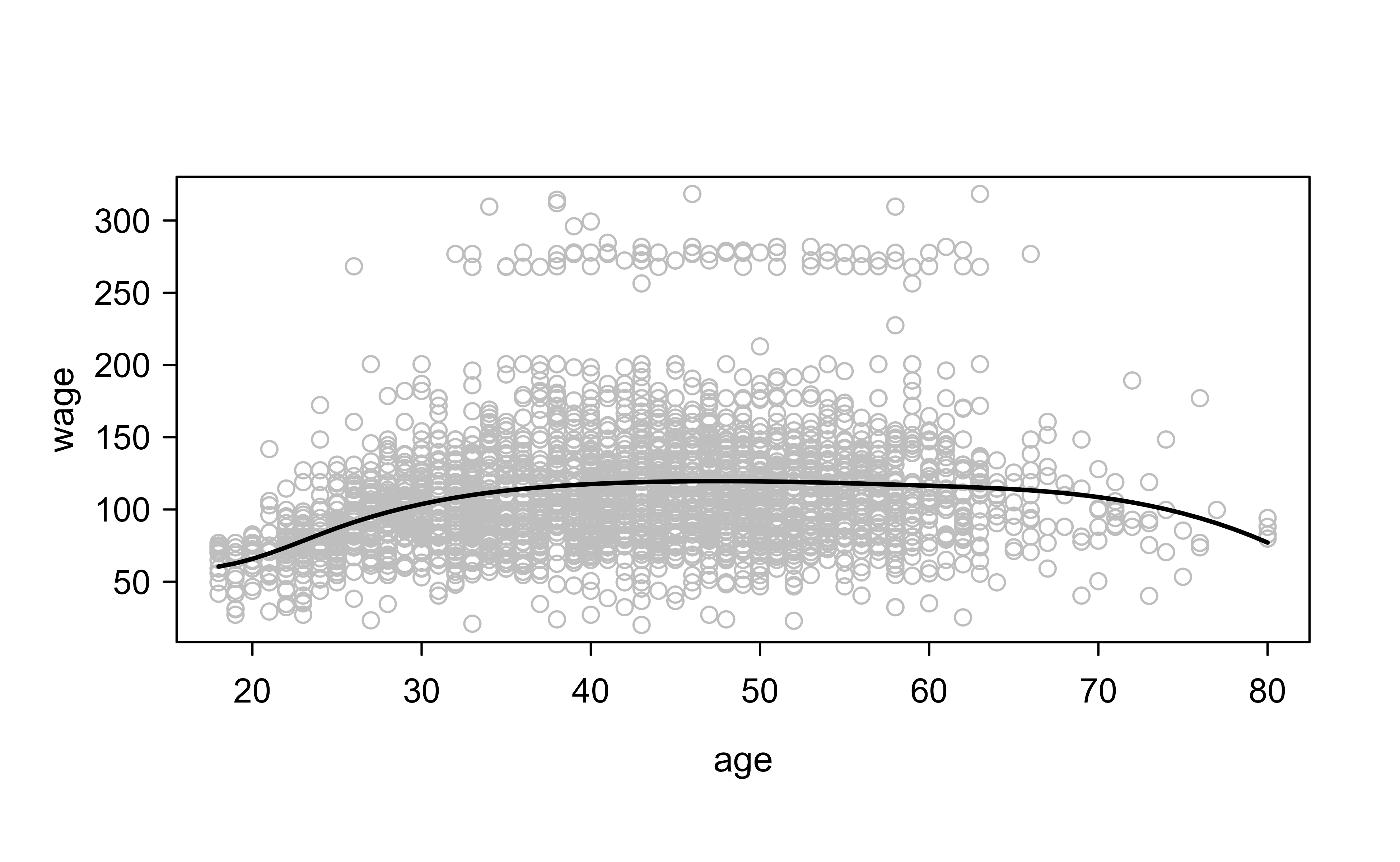
We start with a cubic regression spline. The function bs() from the splines package builds the B-spline basis columns; passing three interior knots produces six basis functions, so with the intercept the model uses seven degrees of freedom. Figure 3.1 shows the resulting fit.
Show code
library(ISLR2)attach(Wage)library(splines)# using basis functions for splines with the sepcifeid set of knotsfit<-lm(wage~bs(age, knots =c(25, 40, 60)), data =Wage)# 3 knots mean 6 basis function, hence 7 df are used (including the intercept)# we want to predict for a grid of values for ageagelims<-range(age)age.grid<-seq(from =agelims[1], to =agelims[2])pred<-predict(fit, newdata =list(age =age.grid), se =T)plot(age, wage, col ="gray")lines(age.grid, pred$fit , lwd =2)# lines(age.grid, pred$fit + 2 * pred$se, lty = " dashed")# lines(age.grid, pred$fit - 2 * pred$se, lty = " dashed")
Figure 3.1: Cubic regression spline of wage on age fitted with three interior knots at ages 25, 40, and 60. The smooth curve rises through early adulthood, peaks in middle age, and tapers off near retirement.
The fitted curve rises steeply through early adulthood, peaks in middle age, and tapers off afterward, exactly the kind of bend a straight line would miss.
Rather than naming knot locations by hand, we can let bs() choose them at uniform quantiles by specifying the degrees of freedom. The check below confirms that asking for df = 6 yields the same basis dimension and places the knots automatically.
The reported knots fall at the 25th, 50th, and 75th percentiles of age, which is the quantile placement recommended earlier.
3.6.1.2 Natural Spline Example
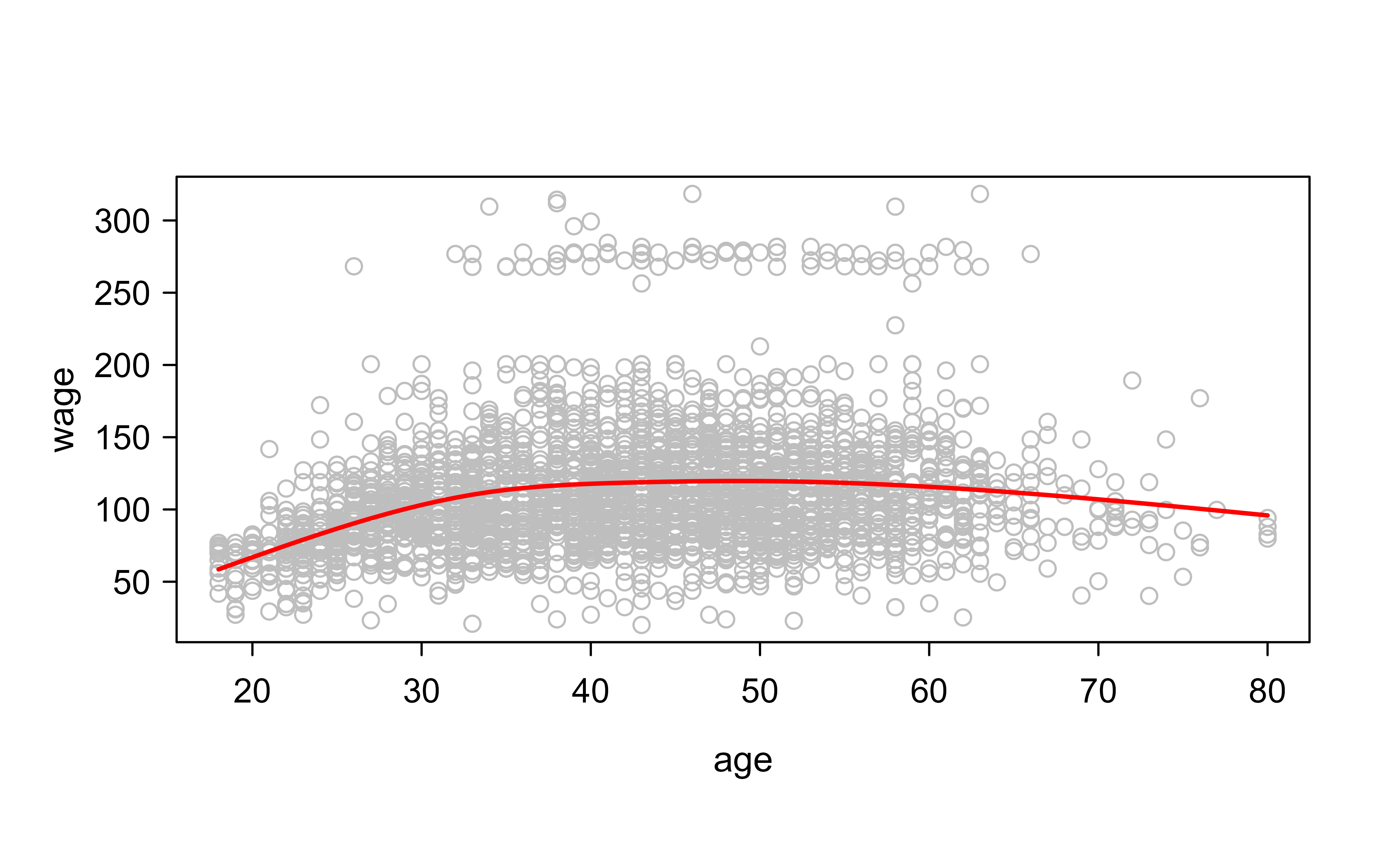
To tame the boundary variance discussed in Natural splines, we switch to ns(), which fits a natural spline (linear beyond the extreme knots). Here df = 4 selects the complexity. Figure 3.2 shows the fit.
Show code
fit2<-lm(wage~ns(age, df =4), data =Wage)# 4 dfpred2<-predict(fit2, newdata =list(age =age.grid), se =T)plot(age , wage , col ="gray")lines(age.grid, pred2$fit, col ="red", lwd =2)
Figure 3.2: Natural cubic spline of wage on age with four degrees of freedom. The fit resembles the regression spline through the bulk of the data but is steadier near the youngest and oldest ages, where the curve is forced to be linear.
The fit looks similar to the regression spline through the bulk of the data but is steadier near the youngest and oldest ages.
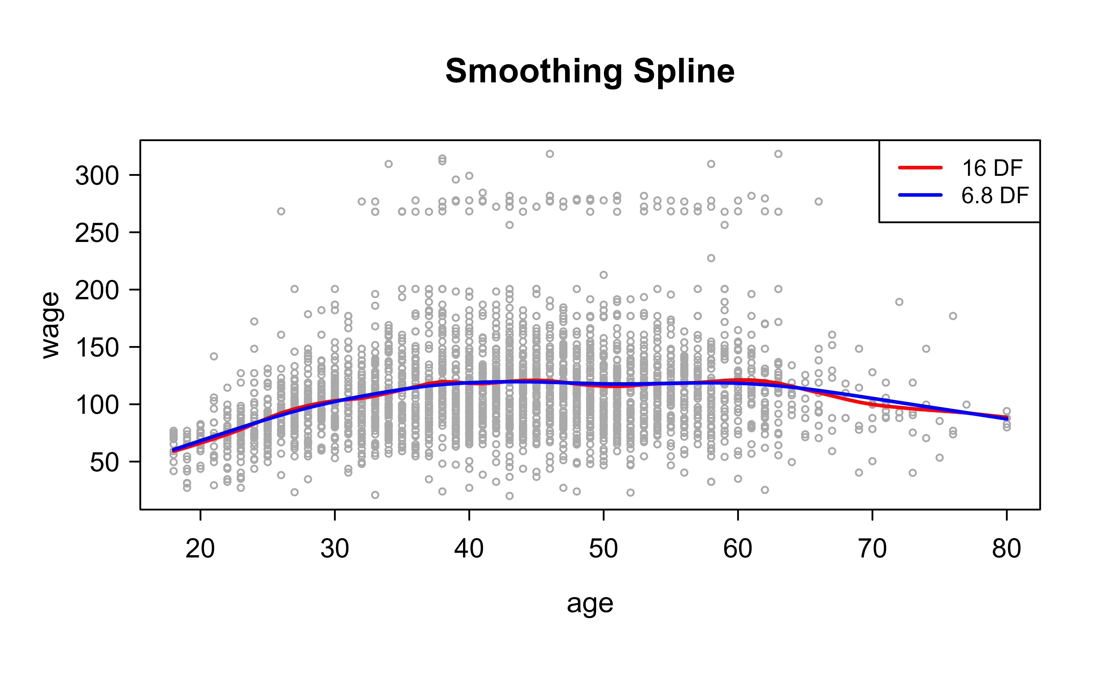
Finally we fit smoothing splines, which place a knot at every distinct age and control flexibility through \(\lambda\). We show two ways to set complexity: fixing the effective degrees of freedom (here 16) and letting R back out the corresponding \(\lambda\), or selecting \(\lambda\) automatically by cross-validation. Figure 3.3 compares the two fits.
Show code
plot(age,wage, xlim =agelims, cex =.5, col ="darkgrey")title("Smoothing Spline")fit<-smooth.spline(age, wage, df =16)# we specify 16 df then R will find lambda that leads to 16 dffit2<-smooth.spline(age, wage , cv =T)# we select lambda (smoothness) based on cross validationfit2$df# wihch result in 6.8 df#> [1] 6.794596lines(fit, col ="red", lwd =2)lines(fit2, col ="blue", lwd =2)legend("topright", legend =c("16 DF", "6.8 DF"), col =c("red", "blue"), lty =1, lwd =2 , cex =.8)
Figure 3.3: Two smoothing splines for wage on age. The red curve fixes the effective degrees of freedom at 16, while the blue curve uses the roughly 6.8 effective degrees of freedom chosen by cross-validation, which is visibly smoother.
Cross-validation chooses about 6.8 effective degrees of freedom, noticeably less flexible than the 16-df curve. The 16-df fit chases more local wiggles, while the cross-validated fit is smoother and likely to generalize better, a concrete illustration of \(\lambda\) trading flexibility for smoothness.
The following short check confirms the eigenvalue identity Equation 3.10 numerically: it builds the smoother matrix \(\mathbf S_\lambda\) for a smoothing spline column by column (each column is the fit to a unit response vector), then verifies that its trace equals the effective degrees of freedom reported by smooth.spline, and that its eigenvalues lie in \([0,1]\) with exactly two equal to one.
Show code
set.seed(1)x<-sort(runif(60))y<-sin(2*pi*x)+rnorm(60, sd =0.3)target_df<-8S<-sapply(seq_along(y), function(i){e<-numeric(length(y)); e[i]<-1predict(smooth.spline(x, e, df =target_df), x)$y})c(trace_S =sum(diag(S)), reported_df =target_df)#> trace_S reported_df #> 8.000957 8.000000ev<-sort(eigen(S, only.values =TRUE)$values, decreasing =TRUE)round(range(ev), 4)# eigenvalues confined to [0, 1]#> [1] 0 1round(ev[1:3], 4)# leading eigenvalues: two unpenalized (= 1), then < 1#> [1] 1.0000 1.0000 0.9966
The trace matches the requested degrees of freedom, and the two leading eigenvalues sit at one (the unpenalized constant and linear directions), exactly as Equation 3.9 predicts.
3.6.2 plot (Example 2)
The second example moves to the Boston data and adds a proper train/test split so we can report out-of-sample performance. We fit a cubic regression spline of medv on lstat with knots at the quartiles, evaluate it on held-out data, and then overlay a smoothing spline for comparison. Table 3.2 reports the held-out accuracy.
Show code
library(tidyverse)library(caret)theme_set(theme_classic())# Load the datadata("Boston", package ="MASS")# Split the data into training and test setset.seed(123)training.samples<-Boston$medv%>%createDataPartition(p =0.8, list =FALSE)train.data<-Boston[training.samples, ]test.data<-Boston[-training.samples, ]knots<-quantile(train.data$lstat, p =c(0.25, 0.5, 0.75))# we use 3 knots at 25,50,and 75 quantile.library(splines)# Build the modelknots<-quantile(train.data$lstat, p =c(0.25, 0.5, 0.75))model<-lm(medv~bs(lstat, knots =knots), data =train.data)# Make predictionspredictions<-model%>%predict(test.data)
Show code
# Model performanceknitr::kable(data.frame( RMSE =RMSE(predictions, test.data$medv), R2 =R2(predictions, test.data$medv)), caption ="Out-of-sample performance of the cubic regression spline of medv on lstat, evaluated on the held-out Boston test set.")
Table 3.2: Out-of-sample performance of the cubic regression spline of medv on lstat, evaluated on the held-out Boston test set.
RMSE
R2
5.317373
0.6786367
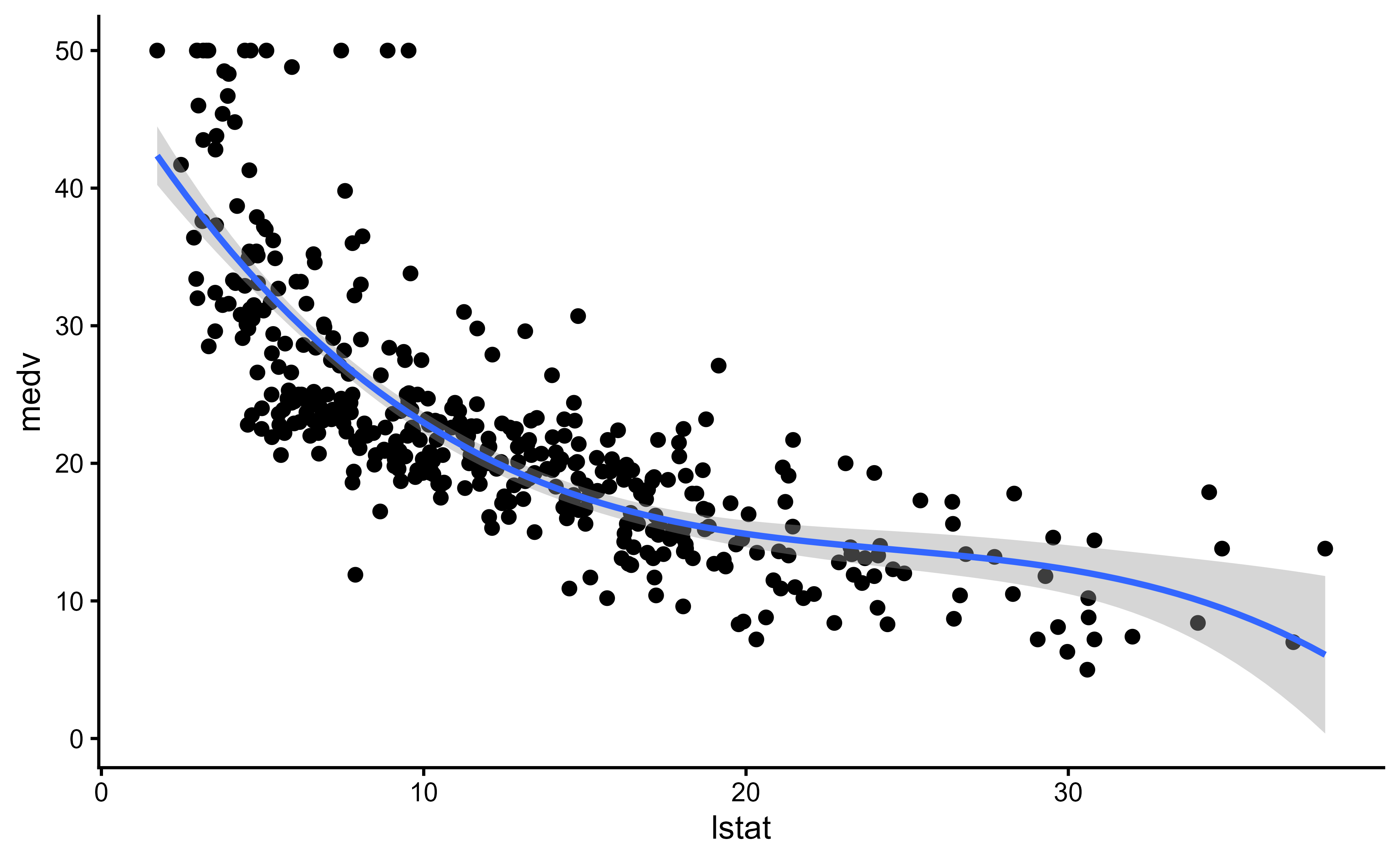
Figure 3.4 shows the regression spline fit with its confidence band over the training data.
Figure 3.4: Cubic regression spline of medv on lstat fitted to the Boston training data, with the shaded pointwise confidence band. The relationship curves downward steeply at low lstat and flattens at high lstat.
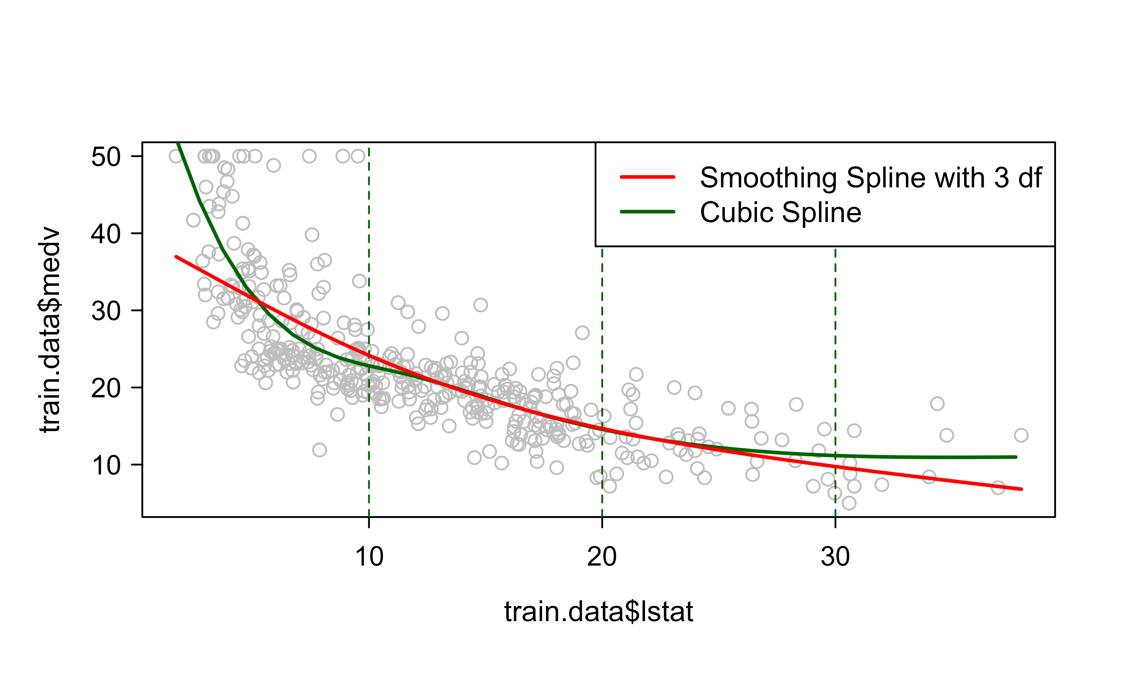
Figure 3.5 overlays the cubic regression spline and a 3-df smoothing spline on the same data.
Show code
attach(train.data)#fitting smoothing splines using smooth.spline(X,Y,df=...)fit1<-smooth.spline(train.data$lstat,train.data$medv,df=3)# 3 degrees of freedom#Plotting both cubic and Smoothing Splinesplot(train.data$lstat,train.data$medv,col="grey")lstat.grid=seq(from =range(lstat)[1], to =range(lstat)[2])points(lstat.grid,predict(model,newdata =list(lstat=lstat.grid)),col="darkgreen",lwd=2,type="l")#adding cutpointsabline(v=c(10,20,30),lty=2,col="darkgreen")lines(fit1,col="red",lwd=2)legend("topright",c("Smoothing Spline with 3 df","Cubic Spline"),col=c("red","darkgreen"),lwd=2)
Figure 3.5: Cubic regression spline (green) and 3-df smoothing spline (red) fitted to the Boston training data. Both track the same downward, curving relationship between lstat and medv, with the dashed vertical lines marking illustrative cut points.
The held-out RMSE and \(R^2\) in Table 3.2 quantify how well the spline generalizes, and the overlay in Figure 3.5 shows the cubic regression spline (green) and the 3-df smoothing spline (red) tracking the same downward, curving relationship between lstat and medv. Both bend where a straight line could not, which is the whole point of this chapter.
When to use this
Reach for splines whenever you suspect a smooth but nonlinear relationship between a predictor and the response and you want a flexible fit that stays interpretable. Use a regression or natural spline when you are comfortable choosing a few knots (or letting quantiles choose them) and want a fast least-squares fit; use a smoothing spline when you would rather not pick knots and prefer to tune a single penalty by cross-validation.
This chapter built every method from one idea, expanding the predictor into a fixed basis and fitting linearly, then controlling complexity either by limiting knots (regression and natural splines) or by penalizing roughness (smoothing and thin-plate splines). The same linear-smoother machinery reappears in local regression (Chapter 5), kernel smoothing (Chapter 4), and, with multiple smooth terms added together, in generalized additive models (Chapter 6).
James, Gareth, Daniela Witten, Trevor Hastie, and Robert Tibshirani. 2013. “Statistical Learning.” In, 15–57. Springer New York. https://doi.org/10.1007/978-1-4614-7138-7_2.
Each \(b_k\) is fixed in advance, not estimated. The only things we estimate are the coefficients that weight them. This is what keeps the fitting step linear.↩︎
# Spline Regression {#sec-spline}```{r}#| include: falsesource("_common.R")```Linear regression assumes that the relationship between a predictor and the response is a straight line. Real data rarely cooperate. Wages rise quickly with age early in a career, then flatten and even decline near retirement; house prices fall steeply as the fraction of lower-income residents rises, then level off. A single straight line cannot capture these bends. We could fit a high-degree polynomial, but global polynomials wiggle wildly near the edges of the data and behave badly when extrapolated. Splines offer a better deal: they bend where the data bend, stay smooth, and keep the variance under control.The idea behind this chapter is a small but powerful shift in perspective. Instead of forcing one rigid functional form on the whole dataset, we build a flexible curve out of simple pieces. Each piece is a low-degree polynomial that governs only a local stretch of the predictor, and we glue the pieces together so the result looks like one smooth curve rather than a chain of disconnected arcs. The points where the pieces meet are called knots, and almost everything interesting about splines comes down to how many knots we use, where we put them, and how strictly we enforce smoothness at them.We approach this through the language of basis functions, which is the unifying thread for everything that follows (and for much of nonparametric regression more broadly). A basis function is just a fixed transformation of the input. Once we choose a good set of these transformations, fitting a curved relationship reduces to ordinary least squares on the transformed columns. That is the practical payoff: the hard nonlinear problem becomes a familiar linear one.By the end of the chapter you will be able to read and interpret four closely related tools: regression splines (piecewise polynomials with a chosen number of knots), natural splines (regression splines tamed at the boundaries), smoothing splines (which place a knot at every observation and control flexibility with a penalty), and multidimensional splines (the same ideas in two or more predictors). These methods connect directly to local regression (@sec-local) and kernel smoothing (@sec-kernel), which we treat as different routes to the same destination: a smooth estimate of $E(Y \mid X = x)$.## Basis Function Representations {#sec-basis-function-representations}The starting point for all spline methods is the observation that we can describe a curved function as a weighted sum of simpler, fixed building blocks. Each building block is called a basis function, and choosing the right collection of them is what gives a model its flexibility.Let the k-th basis function of X be denoted by $b_k(X), k = 1,\dots, K$ which is function that maps from the p-dimensional real numbers to the real line.^[Each $b_k$ is fixed in advance, not estimated. The only things we estimate are the coefficients that weight them. This is what keeps the fitting step linear.]Then, the linear functional representation of $f(X)$ given by these basis functions is$$f(X) = \beta_0 + \sum_{k=1}^K \beta_k b_k(X)$$Equivalently$$\mathbf{Y} = \mathbf{B} \beta + \mathbf{\epsilon}$$where $\mathbf{B}$ is the $n \times (K+1)$ matrix columns given by a vector of 1 for the intercept and $\mathbf{b}_k =(b_k(x_1), \dots, b_k (x_n))', k = 1, \dots, K$::: {.callout-important title="Key idea"}Once the basis functions are chosen, the model is linear in the coefficients $\beta$. So even though $f(X)$ may be highly curved in $X$, we estimate it with the same machinery as ordinary least squares applied to the transformed design matrix $\mathbf{B}$.:::Because the model is linear in $\beta$, the least squares solution has the familiar closed form:$$\hat{\beta} = (\mathbf{B}^T \mathbf{B})^{-1} \mathbf{B}^T\mathbf{y}$$if the basis functions are orthogonal, then we have a special case $\hat{\beta} = \mathbf{B}^T \mathbf{y}$### Why the fit is a linear smoother {#sec-spline-linear-smoother}It is worth making the structure of the fitted values explicit, because it recurs for every method in this chapter. Plugging $\hat\beta$ back into $\hat{\mathbf{y}} = \mathbf{B}\hat\beta$ gives$$\hat{\mathbf{y}} = \mathbf{B}(\mathbf{B}^T\mathbf{B})^{-1}\mathbf{B}^T \mathbf{y} = \mathbf{H}\,\mathbf{y},\qquad \mathbf{H} = \mathbf{B}(\mathbf{B}^T\mathbf{B})^{-1}\mathbf{B}^T,$$ {#eq-spline-hatmatrix}so the fit is a fixed linear map $\mathbf{H}$ applied to the responses. For an unpenalized regression spline $\mathbf{H}$ is the orthogonal projection onto the column space of $\mathbf{B}$, hence idempotent ($\mathbf{H}^2 = \mathbf{H}$) and symmetric, with $\operatorname{tr}(\mathbf{H}) = K+1$ equal to the number of basis columns. The trace counting the model dimension is the seed of the effective-degrees-of-freedom idea that returns for smoothing splines, where $\mathbf{H}$ is no longer a projection but the trace still measures complexity.Under the standard regression assumptions $E(\mathbf{y}) = \mathbf{f}$ (the vector of true regression values $f(x_i)$) and $\operatorname{Var}(\mathbf{y}) = \sigma^2 \mathbf{I}$, the pointwise variance and bias of the fit follow immediately from linearity. With $\mathbf{h}(x)^T = b(x)^T(\mathbf{B}^T\mathbf{B})^{-1}\mathbf{B}^T$ the row of the smoother that produces $\hat f(x)$,$$\operatorname{Var}\!\big(\hat f(x)\big) = \sigma^2\,\lVert \mathbf{h}(x)\rVert_2^2,\qquad\operatorname{Bias}\!\big(\hat f(x)\big) = \mathbf{h}(x)^T \mathbf{f} - f(x).$$ {#eq-spline-biasvar}For a fixed basis the variance is exactly linear in $\sigma^2$ and grows with the number of columns, while the bias is whatever the projection of the true function onto the span of the basis leaves behind. Adding knots shrinks the bias (the span gets richer) and inflates the variance (more columns, larger $\lVert\mathbf{h}(x)\rVert$), which is the bias-variance tradeoff in its most transparent form. This is the formal content behind the informal statement, made later, that more knots mean more flexibility.Many models you already know are just particular choices of basis functions. The following list shows how familiar ideas all fit under this one umbrella:- Original linear model: $b_k(X) = X_k, k = 1, \dots, p$- Polynomials: $b_k(X) = X^2_j; X^3_j; X_jX_m$- Non-linear transformations: $b_k(X)= \log(X_j); \sqrt{X_j}$- Step-functions: $b_k(X) = I(c_k \le X \le v_k)$, an indicator for a region of $X$ 1. Breaking the region up into non-overlapping regions and step-function response 2. Example: for a single $X$, $b_0 (X) = I(X < c_1), \dots, b_{K-1}(X) = I(c_{K-1} \le X \le c_K)$ where $c_1, \dots, c_k$ are cut points (i.e., making dummy variables and piece wise constant regression fits)- Other: sines and cosines, wavelets, empirical basis functionsThe step-function basis in particular is worth holding onto, because it is the crudest version of the spline idea: chop the range of $X$ into regions and fit a separate constant in each. Splines refine this by replacing the constants with low-degree polynomials and by demanding that the pieces join smoothly.<br>With that intuition in place, we can give the formal definition. (A careful derivation of what follows can be found on CMU stat^[<https://www.stat.cmu.edu/~ryantibs/advmethods/notes/smoothspline.pdf>].)Definition: a k-th order spline is a piecewise polynomial function of degree k, that is continuous and has continuous derivatives of orders 1,..., k -1, at its knot pointsEquivalently, a function f is a k-th order spline with knot points at $t_1 < ...< t_m$ if the two conditions below hold together:- f is a polynomial of degree k on each of the intervals $(-\infty, t_1], [t_1,t_2],...,[t_m, \infty)$\- $f^{(j)}$, the j-th derivative of f, is continuous at $t_1,...,t_m$ for each j = 0,1,...,k-1The first condition says the curve is built from polynomial pieces; the second says the seams between pieces are invisible up through the $(k-1)$-th derivative, which is what makes the joins look smooth rather than kinked.A common case is when k = 3, called cubic splines. (piecewise cubic functions are continuous, and also continuous at its first and second derivatives) Cubic splines are the default in practice because the human eye cannot detect discontinuities beyond the second derivative, so going higher buys nothing visible.To parameterize the set of splines, we could use truncated power basis, defined as$$g_1(x) = 1 \\g_2(x) = x \\... \\g_{k+1}(x) = x^k \\g_{k+1+j}(x) = (x-t_j)^k_+$$where j = 1,...,m and $x_+$ = max{x,0}The first $k+1$ functions reproduce an ordinary polynomial; each extra term $(x - t_j)^k_+$ switches on only past the knot $t_j$, adding exactly the flexibility needed to bend the curve there without breaking smoothness.::: {.callout-warning}The truncated power basis is easy to understand but numerically unstable, because its columns become highly correlated. Software typically uses the equivalent but better-conditioned B-spline basis instead. The fitted curve is the same; only the internal parameterization differs.:::## Regression SplinesA regression spline is the practical workhorse of this chapter: you pick a degree, pick a handful of knots, build the corresponding basis columns, and run ordinary least squares. It sits squarely between two simpler ideas, polynomial regression and piecewise constant regression, borrowing the local flexibility of the latter and the smoothness of the former.The construction is easiest to see by first writing down what we would get without any smoothness constraints. Suppose we split the range of $X$ at a single knot $c$ and fit a separate cubic on each side:$$y_i =\begin{cases}\beta_{01} + \beta_{11}x_i + \beta_{21}x_i^2 + \beta_{31}x_i^3+ \epsilon & \text{if } x_i <c\\\beta_{02}+\beta_{12}x_i +\beta_{22}x_i^2+\beta_{32}x_i^3+\epsilon &\text{if } x_i \ge c\end{cases}$$where $c$ is a knot point. As written, these two cubics are completely free, so the fitted curve can jump and kink at $c$. The flexibility of the model grows with the number of knots: the more knots we add, the more local wiggles the curve can follow.If we have $K$ knots through the range of $X$, we fit $K+1$ different (cubic or any or constants) polynomials. Left alone, those pieces would not connect. We fix this by adding constraints, one at a time:- To restrict piece coming together at the knot points, we add the constraint that the fitted curve must be continuous.- We constrain the first and second derivatives to be continuous for smoothness.If the polynomials are cubic, then it's cubic spline.::: {.callout-tip title="Intuition"}Each constraint is a deal: you give up a degree of freedom in exchange for a smoother curve. A free piecewise cubic with $K$ knots would have $4(K+1)$ parameters, but the continuity and derivative constraints knock most of them out. Each constraint that we add reduces the number of parameters to be fit (frees up df), and less complex.:::After all the constraints, a cubic spline with $K$ knots has $K +4$ df.::: {.callout-note title="Deriving the degree-of-freedom count"}The arithmetic behind "$K+4$" is worth doing once. With $K$ interior knots the predictor range is split into $K+1$ intervals, and a free cubic on each interval has $4$ coefficients, for $4(K+1)$ parameters in total. At each of the $K$ knots we impose continuity of the function and of its first and second derivatives, that is $3$ constraints per knot, or $3K$ constraints. The dimension of the resulting function space is$$4(K+1)-3K=4K+4-3K=K+4.$${#eq-spline-dfcount}The same logic gives $(k+1)(K+1)- kK =K+ k +1$ for a spline of degree $k$, which matches the truncated-power count $m + k +1$ used below (with $m =K$ knots). Each derivative-continuity constraint removes exactly one degree of freedom, the precise meaning of the earlier "each constraint is a deal.":::We can rewrite the cubic spline into the general basis notation, which is exactly the truncated power basis specialized to cubics:$$b_1(X) =X; b_2(X) =X^2; b_3(X) =X^3; b_4(X) =h(X,\xi_1);\\b_5(X) =h(X,\xi_2) ,\dots, b_{K+3} (X) =h(X,\xi_K)$$where$$h(x,\xi) =(x-\xi)^3_+=\begin{cases}(x- \xi)^3&\text{if } x > \xi \\0 & \text{otherwise}\end{cases}$$and $\xi$ is the knot. Fitting this model with an intercept requires estimating $K+4$ regression coefficients (i.e., $K +4$ df).This basis representation is the bridge from theory to code: the $b_k(X)$ become the columns of the design matrix, and the fit is plain least squares. Two practical issues remain, behavior at the edges and the choice of knots.- Splines have high variance at the outer range of the predictors. - [Natural splines] are regression splines with extra constrains on the boundary that mitigates this variance problem by requiring the function to be linear in the regions where $X$ is smaller than the smallest knot, and larger than the largest knot. - To decide number and place of knots ($K$) - To choose number of $K$, people usually do cross-validation - Given $K$ knots, we locate them uniformly in the quantile domain of $X$ - Ex: $K = 3$, a knot would be placed at the 25th, 50th, and 75th percentiles of the variable X. - Alternatively, we can place knots based on local data abundance.::: {.callout-tip}Placing knots at quantiles (rather than evenly along the axis) puts more knots where you have more data, so the model spends its flexibility where it can actually learn something and avoids straining in sparse regions.:::<br>It helps to see the same construction written in the more general notation used in the smoothing-spline literature, because we will reuse it shortly. To estimate the regression function $r(X) = E(Y|X =x)$, we can fit a k-th order spline with knots at some prespecified locations $t_1,...,t_m$.Regression splines are functions of$$\sum_{j=1}^{m+k+1} \beta_jg_j$$where $\beta_1,..\beta_{m+k+1}$ are coefficients and $g_1,...,g_{m+k+1}$ are the truncated power basis functions for k-th order splines over the knots $t_1,...,t_m$.To estimate the coefficients we minimize the usual sum of squared residuals:$$\sum_{i=1}^{n} (y_i - \sum_{j=1}^{m+k+1} \beta_j g_j (x_i))^2$$then regression spline is$$\hat{r}(x) = \sum_{j=1}^{m+k+1} \hat{\beta}_j g_j (x)$$If we define the basis matrix $G \in R^{n \times (m+k+1)}$ by$$G_{ij} = g_j(x_i)$$where $i = 1,..,n$ , $j = 1,..,m+k+1$Then the objective is just least squares in disguise,$$\sum_{i=1}^{n} (y_i - \sum_{j=1}^{m+k+1} \beta_j g_j (x_i))^2 = ||y - G \beta||_2^2$$and the regression spline estimate at x is$$\hat{r} (x) = g(x)^T \hat{\beta}= g(x)^T(G^TG)^{-1}G^Ty$$which is the same closed-form solution from @sec-basis-function-representations, now with $G$ playing the role of $\mathbf{B}$.## Natural splinesThe boundary-variance problem flagged above motivates the natural spline. The fix is simple to state: instead of letting the polynomial pieces run free past the outermost knots, we force the function to be linear out there, where data are scarce and a high-degree fit would otherwise swing wildly.A natural spline of order k, with knots at $t_1 <...< t_m$, is a piecewise polynomial function f such that- f is polynomial of degree k on each of $[t_1,t_2],...,[t_{m-1},t_m]$- f is a polynomial of degree $(k-1)/2$ on $(-\infty,t_1]$ and $[t_m,\infty)$- f is continuous and has continuous derivatives of orders 1,.,,, k -1 at its knots $t_1,..,t_m$The middle condition is the heart of it: for a cubic ($k = 3$), the boundary degree is $(3-1)/2 = 1$, so the curve becomes a straight line beyond the extreme knots. This trades a little flexibility for much narrower confidence bands at the edges.### Boundary constraints and the degrees-of-freedom saving {#sec-natural-spline-df}For a cubic the linearity beyond the extreme knots is equivalent to four derivative constraints, two at each boundary knot:$$f''(t_1) = 0, \quad f'''(t_1) = 0, \qquad f''(t_m) = 0, \quad f'''(t_m) = 0 .$$ {#eq-spline-natural-bc}Beyond $t_1$ and $t_m$ a cubic that is to continue as a straight line must have vanishing second and third derivatives there, and continuity up to the second derivative then forces those same conditions on the interior cubic at the boundary knots. A cubic regression spline with $m$ knots has $m+4$ degrees of freedom; imposing the four conditions in @eq-spline-natural-bc removes four, leaving$$(m + 4) - 4 = m,$$ {#eq-spline-natural-dfcount}so a natural cubic spline has exactly $m$ degrees of freedom, one per knot. This is why `ns(age, df = 4)` corresponds to four knots (here counting the two boundary knots), whereas `bs(age, df = 6)` with a cubic needs three interior knots to reach six basis columns: the natural spline spends its budget more frugally, which is precisely the variance reduction at the edges paid for in flexibility.::: {.callout-note title="Why the variance drops at the boundary"}Recall from @eq-spline-biasvar that $\operatorname{Var}(\hat f(x)) = \sigma^2\lVert\mathbf{h}(x)\rVert_2^2$. Near the edges of the data an unconstrained cubic spline has few observations to anchor its highest-order behavior, so the weight vector $\mathbf{h}(x)$ has large norm and the variance balloons. Forcing linearity past the extreme knots collapses the local model from a cubic (four local parameters) to a line (two), shrinking $\lVert\mathbf{h}(x)\rVert$ and hence the boundary variance. The price is bias if the truth is genuinely curved in the tails, but data are usually too sparse there to detect such curvature reliably.:::::: {.callout-note}Natural splines are only defined for odd orders k, because the boundary degree $(k-1)/2$ must be an integer. Cubic ($k=3$) is the standard choice.:::## Smoothing splinesRegression splines make you choose the number and location of knots. Smoothing splines sidestep that choice entirely with a clever move: put a knot at every distinct observation, then prevent overfitting not by limiting knots but by penalizing roughness directly.We are interested in a function $g(x)$ and try to minimize $RSS = \sum_{i=1}^n (y_i -g(x_i))^2$.But we wouldn't want to overfit (because $g(x)$ that minimizes this RSS will try to interpolate all of the $y_i$), then we want to a smooth $g(x)$ that minimizes RSS:$$\sum_{i=1}^n (y_i - g(x_i))^2 + \lambda \int g''(x)^2\, dx$$where- $\lambda$ is a non-negative smoothness- $g(.)$ is a smoothing splineThe objective has two competing parts, and reading them in plain words makes the method intuitive:- RSS here is a *loss function* that rewards fitting the data closely.- The second term is a *smoothness penalty term* that rewards a gently curving function. - Second derivative controls the smoothness of the function (smaller in absolute value means smoother). The second derivative measures how fast the slope is changing, so penalizing its size discourages sharp bends. - Parameter $\lambda$ controls the tradeoff between the smoothness and fit.The single tuning knob $\lambda$ slides the fit between the two extremes:- When $\lambda = 0$, the penalty is inactive and $g$ is the maximally flexible interpolant (a natural cubic spline through every point, $df = n$).- When $\lambda \to \infty$, $g$ approaches the ordinary least squares straight line (the smoothest possible fit, $df = 2$), which best fits but does not interpolate the data.::: {.callout-important title="Key idea"}Although we nominally place a knot at every data point, the penalty does the real work. The remarkable fact is that the function minimizing the penalized objective is exactly a natural cubic spline with knots at the unique observed values of $x$.:::### Why the minimizer is a natural cubic spline {#sec-smoothing-spline-derivation}The penalized objective is stated over an infinite-dimensional function space (all functions with square-integrable second derivative, the Sobolev space $W^2_2$), yet its minimizer is a finite-dimensional object. The standard argument runs as follows. Suppose $\tilde g$ is any competing function passing through the fitted points, that is $\tilde g(x_i) = g(x_i)$ for all $i$, where $g$ is the natural cubic spline interpolating those same values. Both functions then have identical data-fit terms, so they can only differ in the penalty. Writing $h = \tilde g - g$, integration by parts on each interknot interval together with the natural boundary conditions $g''(t_1) = g''(t_m) = 0$ from @eq-spline-natural-bc gives$$\int g''(x)\, h''(x)\, dx= \big[ g''(x) h'(x)\big]_{t_1}^{t_m} - \int g'''(x)\, h'(x)\, dx= - \int g'''(x)\, h'(x)\, dx .$$Because $g$ is a natural cubic spline, $g'''$ is piecewise constant and vanishes outside $[t_1, t_m]$, so a further integration by parts on each interval (using $h(t_i) = 0$) makes this last integral vanish. Hence $\int g'' h'' \,dx = 0$, and$$\int \tilde g''(x)^2\, dx= \int g''(x)^2 \, dx + 2\!\int g''(x) h''(x)\,dx + \int h''(x)^2\, dx= \int g''(x)^2\,dx + \int h''(x)^2\,dx\;\ge\; \int g''(x)^2\, dx ,$$ {#eq-spline-ncs-optimality}with equality only if $h'' \equiv 0$. So among all functions interpolating a given set of fitted values, the natural cubic spline has the smallest roughness penalty. Since the data-fit term depends only on the values at the $x_i$, the global minimizer of the penalized criterion must itself be a natural cubic spline with knots at the unique $x_i$. This is the rigorous content of the "Key idea" above, and it is what reduces the infinite-dimensional problem to a finite regression.### The penalized least-squares solution {#sec-reinsch}Once we know the answer lives in the natural-spline space, expand $g(x) = \sum_{j=1}^{n} \beta_j N_j(x)$ in a natural cubic spline basis $\{N_j\}$ with $\{\mathbf N\}_{ij} = N_j(x_i)$ and penalty matrix $\{\boldsymbol\Omega_N\}_{jk} = \int N_j''(t) N_k''(t)\,dt$. The criterion becomes a finite generalized-ridge problem,$$\operatorname*{arg\,min}_{\beta}\; \lVert \mathbf y - \mathbf N \beta\rVert_2^2 + \lambda\, \beta^T \boldsymbol\Omega_N \beta .$$ {#eq-spline-penalized-objective}Setting the gradient to zero,$$-2\mathbf N^T(\mathbf y - \mathbf N\beta) + 2\lambda\,\boldsymbol\Omega_N \beta = 0\;\Longrightarrow\;(\mathbf N^T\mathbf N + \lambda\,\boldsymbol\Omega_N)\,\hat\beta = \mathbf N^T\mathbf y ,$$so $\hat\beta = (\mathbf N^T\mathbf N + \lambda\,\boldsymbol\Omega_N)^{-1}\mathbf N^T\mathbf y$ and the fitted values are $\hat{\mathbf y}_\lambda = \mathbf N\hat\beta = \mathbf S_\lambda \mathbf y$ with$$\mathbf S_\lambda = \mathbf N(\mathbf N^T\mathbf N + \lambda\,\boldsymbol\Omega_N)^{-1}\mathbf N^T ,$$ {#eq-spline-smoother-derived}which is exactly the smoother matrix quoted later from @hastie2001a. The penalty is a generalized ridge: it shrinks not the raw coefficients but the directions that produce roughness, leaving the linear and constant components (for which $N_j'' = 0$, hence in the null space of $\boldsymbol\Omega_N$) completely unpenalized. This is why $\lambda\to\infty$ drives the fit to the ordinary least squares line rather than to zero: only the rough part is annihilated.### Eigen-analysis and the limits of $\lambda$ {#sec-spline-eigen}The shrinkage structure becomes transparent in the Demmler-Reinsch basis. The smoother $\mathbf S_\lambda$ is symmetric (it can be written $\mathbf S_\lambda = (\mathbf I + \lambda \mathbf K)^{-1}$ where $\mathbf K = \mathbf N^{-T}\boldsymbol\Omega_N \mathbf N^{-1}$ is the penalty in the value parameterization), so it admits a real eigendecomposition $\mathbf S_\lambda = \sum_{k=1}^{n} \rho_k(\lambda)\, \mathbf u_k \mathbf u_k^T$ with eigenvectors $\mathbf u_k$ independent of $\lambda$ and eigenvalues$$\rho_k(\lambda) = \frac{1}{1 + \lambda\, d_k}, \qquad d_k \ge 0 ,$$ {#eq-spline-eigenvalues}where $d_k$ are the eigenvalues of $\mathbf K$. Two of the $d_k$ are zero (the constant and linear eigenvectors), so those components are never shrunk, $\rho_k = 1$. The remaining eigenvectors are ordered by increasing roughness, and the corresponding $\rho_k$ decay toward zero: a smoothing spline is a soft, frequency-graded shrinker, damping wiggly components more than smooth ones, in contrast to a regression spline whose hat matrix has eigenvalues that are exactly $0$ or $1$. The effective degrees of freedom are the sum of these eigenvalues,$$df_\lambda = \operatorname{tr}(\mathbf S_\lambda) = \sum_{k=1}^{n} \frac{1}{1 + \lambda\, d_k} ,$$ {#eq-spline-df-eigen}a smooth, strictly decreasing function of $\lambda$. The endpoints quoted earlier now drop out by inspection: as $\lambda\to 0$ every $\rho_k\to 1$ and $df_\lambda \to n$ (interpolation), while as $\lambda\to\infty$ all but the two unpenalized eigenvalues vanish and $df_\lambda \to 2$ (the OLS line). Equation @eq-spline-df-eigen is also the practical device for converting a target $df$ into a $\lambda$, which is what `smooth.spline(..., df = 16)` solves numerically.The properties below summarize why this works and how to think about model complexity here:- The smoothing spline function corresponds to a cubic polynomial basis with knots at the unique values of $x_1, \dots, x_n$ with continuous first and second derivatives at each knot 1. $g(x)$ that minimizes the smoothing spline constraint is just a natural cubic spline with knots at the unique $x$ observations 2. $\lambda$ controls the level of shrinkage for smoothing splines, but there is none in regression spline 3. At first glance, we might think that smoothing splines might have too many degrees of freedom since we have knots at every data points (i.e., $K = n$). But $\lambda$ controls roughness and make the effective degrees of freedom much smaller (as $\lambda$ increases from $0 \to \infty$, $df_\lambda$ decreases from $n \to 2$)That last point introduces a key quantity, the effective degrees of freedom, which lets us talk about the complexity of a penalized fit even though we are not literally counting free parameters. To define it, note that the fitted values are a linear function of the responses.Let $\hat{\mathbf{y}}_\lambda$ be the n-vector containing the fitted values for the smoothing spline function for a given $\lambda$, then$$\hat{\mathbf{y}}_\lambda = \mathbf{S}_\lambda \mathbf{y}$$which means that it is linear in $\mathbf{y}$.According to @hastie2001a (section 5.4) showed$\mathbf{S}_\lambda = \mathbf{N}(\mathbf{N}^T\mathbf{N}+ \lambda \mathbf{\Omega}_N)^{-1} \mathbf{N}^T$ where $\{N\}_{ij} = b_j (x_i)$ and$\{\mathbf{\Omega}\}_{jk} = \int b''_j (t) b''_k(t)dt$The matrix $\mathbf{S}_\lambda$ acts on $\mathbf{y}$ to produce a smoothed version of it, so it is called the smoother matrix. Its trace counts the effective degrees of freedom:$$df_\lambda = \sum_{i=1}^n \{\mathbf{S}_\lambda\}_{ii}$$(the trace plays the same role here that the number of fitted coefficients plays in ordinary regression). $\mathbf{S}_\lambda$ is related to other types of smoothing in local regression (@sec-local) and kernel smoothing (@sec-kernel), which all share this linear-smoother structure.<br>This linear structure also gives a fast way to tune $\lambda$. To choose $\lambda$, we can use cross-validation (and we can also use the relationship between $\lambda$ and effective degrees of freedom). The convenient part is that for any linear smoother, leave-one-out cross-validation has a shortcut that avoids refitting:$$\begin{aligned}RSS_{CV}(\lambda)&= \sum_{i=1}^n(y_i - \hat{y}_\lambda^{(-i)}(x_i))^2 \\&= \sum_{i=1}^n[\frac{y_i - \hat{y}_\lambda(x_i)}{1-\{\mathbf{S}_\lambda\}_{ii}}]^2\end{aligned}$$where we only have to fit the model once for each $\lambda$. This is why the diagonal of $\mathbf{S}_\lambda$ is worth computing: it gives both the effective degrees of freedom and the leave-one-out error in one shot.A robust and slightly cheaper alternative replaces each diagonal element by their average, giving generalized cross-validation (GCV),$$GCV(\lambda) = \frac{1}{n}\sum_{i=1}^n\left[\frac{y_i - \hat y_\lambda(x_i)}{1 - \operatorname{tr}(\mathbf S_\lambda)/n}\right]^2= \frac{n\,\lVert \mathbf y - \mathbf S_\lambda \mathbf y\rVert_2^2}{(n - df_\lambda)^2} ,$$ {#eq-spline-gcv}which depends on $\mathbf S_\lambda$ only through the trace $df_\lambda$ and is invariant to orthogonal rotations of the response, making it more stable than LOOCV when some $\{\mathbf S_\lambda\}_{ii}$ approach one.### Asymptotic properties and the equivalent kernel {#sec-spline-asymptotics}Smoothing splines are not merely convenient; they are rate-optimal nonparametric estimators. If the true regression function $f$ has $m$ square-integrable derivatives and the penalty is on the $m$-th derivative (the case $m=2$ is the cubic smoothing spline), then with $\lambda \asymp n^{-2m/(2m+1)}$ the integrated mean squared error attains$$\int E\big(\hat f(x) - f(x)\big)^2\, dx = O\!\left(n^{-2m/(2m+1)}\right) ,$$ {#eq-spline-rate}which is the minimax-optimal rate over the corresponding smoothness class. For cubic smoothing splines ($m=2$) this is $O(n^{-4/5})$, the same rate achieved by local linear regression and by kernel smoothing with an optimal bandwidth, which is the precise sense in which these methods are "different routes to the same destination." The optimal $\lambda$ balances a squared bias of order $\lambda$ against a variance of order $(n\lambda^{1/4})^{-1}$ in the interior, and the rate follows from minimizing their sum.This equivalence is more than a shared rate. @hastie2001a (the Green-Silverman result) show that for large $n$ the smoothing-spline weight function behaves like a kernel: away from the boundary the rows of $\mathbf S_\lambda$ are approximately$$\hat f(x) \approx \frac{1}{n}\sum_{i=1}^n \frac{1}{p(x)\,h(x)}\,K_{\mathrm{eq}}\!\left(\frac{x_i - x}{h(x)}\right) y_i ,\qquadK_{\mathrm{eq}}(u) = \tfrac12 \exp\!\big(-|u|/\sqrt 2\big)\sin\!\big(|u|/\sqrt 2 + \pi/4\big) ,$$ {#eq-spline-equivkernel}where $p(x)$ is the design density and the local bandwidth scales as $h(x) \propto \big(\lambda / (n\,p(x))\big)^{1/4}$. Two facts make this revealing. First, the equivalent kernel adapts its bandwidth to the local data density automatically, putting more smoothing where data are sparse, which is exactly the behavior we engineered by hand with quantile knot placement. Second, the "Silverman kernel" $K_{\mathrm{eq}}$ is fixed and has the same form regardless of $\lambda$, so a smoothing spline is, asymptotically, a kernel smoother in disguise, formalizing @tbl-spline-tuning-comparison.### Practical guidance: choosing complexity and reading diagnostics {#sec-spline-howto}The hyperparameters and how to set them are method-specific, but the logic is shared.- Number and placement of knots (regression and natural splines). Prefer to specify a target $df$ and let the software place knots at quantiles of $x$, as in `bs(age, df = 6)` and `ns(age, df = 4)`. Quantile placement (rather than equispaced) is the safe default because it allocates flexibility in proportion to data density; equispaced knots can leave a sparse region underconstrained and oversmooth a dense one. The fit is fairly insensitive to exact knot positions once there are enough of them, and quite sensitive to the count, so spend tuning effort on $df$ via cross-validation, not on hand-tuning locations.- Smoothing parameter (smoothing splines). Tune $\lambda$ through $df_\lambda$ using GCV (@eq-spline-gcv) or LOOCV (@eq-spline-gcv is computed in one pass via the trace). Reporting $df_\lambda$ rather than $\lambda$ itself is recommended because it is interpretable and scale-free: a fit with $df_\lambda = 6.8$ is comparable across datasets, whereas the raw $\lambda$ is not. GCV occasionally undersmooths; if the curve looks visibly noisy, cap $df_\lambda$ or switch to REML-based selection.- Computational cost. The matrices $\mathbf N^T\mathbf N$ and $\boldsymbol\Omega_N$ for a cubic smoothing spline are banded (each $N_j$ has local support), so the linear system in @eq-spline-smoother-derived solves in $O(n)$ time by the Reinsch algorithm, not the $O(n^3)$ a dense solve would cost. Regression splines with $K$ fixed knots cost $O(nK^2)$ to fit, independent of how finely the curve is later evaluated.- Diagnostics and failure modes. Plot the fit with its pointwise band (@eq-spline-biasvar); fanning bands at the edges signal the boundary variance that natural splines are meant to cure. Watch for oscillation between knots (too many knots or too small $\lambda$) and for systematic lack of fit in a curved region (too few knots or too large $\lambda$). Splines extrapolate poorly: outside the data range a regression spline continues as an unconstrained cubic and a natural spline as a line, neither of which is trustworthy, so confine predictions to the observed support of $x$.## Multidimensional SplinesSo far $X$ has been a single predictor. When the response depends smoothly on two or more inputs at once, we build higher-dimensional curves by multiplying one-dimensional basis functions together, an operation called the tensor product.We can extend the above one-dimensional spline models to higher dimensions using tensor products to form higher dimensional basis functions.Consider $X \in R^2$ and- basis functions $b_{1j}(X_1), j = 1, \dots, K_1$ for representing coordinate $X_1$- $b_{2k}(X), k = 1, \dots, K_2$ for coordinate $X_2$then the *tensor product basis* is:$$g_{jk}(X) = b_{1j}(X_1)b_{2k}(X_2)$$where $j = 1, \dots, K_1, k = 1, \dots, K_2$Each product basis function is large only where both of its one-dimensional factors are large, so it describes a localized bump in the $(X_1, X_2)$ plane. Summing them with coefficients gives the surface:$$f(X) = \sum_{j=1}^{K_1} \sum_{k=1}^{K_2}\beta_{jk}g_{jk}(X)$$::: {.callout-warning}The number of tensor-product basis functions is $K_1 \times K_2$, and it multiplies again with each added dimension. This combinatorial blow-up (a face of the curse of dimensionality) is why pure tensor-product splines are practical mainly for two or three predictors.:::Just as in one dimension, we fit by trading squared error against a roughness penalty. Then, we seek to minimize$$\sum_{i=1}^n (y_i - f(x_i))^2 + \lambda J[f]$$where $J$ is the penalty function for the dimension of the problem.In our example ($X \in R^2$), the penalty integrates the squared second derivatives in every direction, including the cross term:$$J[f] = \int\int[(\frac{\partial^2f(x)}{\partial x_1^2})^2 + 2(\frac{\partial^2 f(x)}{\partial x_1 \partial x_2})^2 + (\frac{\partial^2f(x)}{\partial x^2_2})^2]dx_1 dx_2$$The role of $\lambda$ mirrors the one-dimensional case exactly:- $\lambda \to 0$ gives an interpolating function that goes through all points- $\lambda \to \infty$ gives a solution approaching the least squares plane- We seek a $\lambda$ that compromises between these extremesThis splines method is known as thin-plates splines. The name comes from physics: the penalty measures the bending energy of a thin metal sheet forced to pass near the data, so the fitted surface is the shape the sheet would naturally relax into.<br>Remarkably, the solution to this infinite-dimensional problem has a finite, explicit form. The solution to the thin-plate spline minimization gives$$f(x) = \beta_0 + \beta^T x + \sum_{j=1}^n \alpha_j b_j(x)$$where $b_j(x) = ||x - x_j||^2\log ||x-x_j||$ (known as radial basis functions). Each radial basis function depends only on the distance from a data point $x_j$, so the surface is a smooth plane plus a sum of localized contributions centered at the observations.Additional splines basis functions could be- B-splineLocal regression (@sec-local) and kernel smoothing (@sec-kernel) are related to the spline basis regression formulations, and we recommend reading those chapters alongside this one.<br>As a final unifying view, it is worth seeing smoothing splines written as a single penalized regression, which makes the connection to ridge-type shrinkage explicit. These estimators use a regularized regression over the natural spline basis: placing knots at all points $x_1,...x_n$.For the case of cubic splines, the coefficients are the minimization of$$||y - G\beta||^2_2 + \lambda \beta^T \Omega \beta$$where $\Omega \in R^{n \times n}$ is the penalty matrix$$\Omega_{ij} = \int g''_i(t) g''_j(t) dt,$$and i,j = 1,..,nand $\lambda \beta^T \Omega \beta$ is the regularization term used to shrink the components of $\hat{\beta}$ towards 0. $\lambda > 0$ is the tuning parameter (or smoothing parameter). Higher value of $\lambda$, faster shrinkage (shrinking away basis functions). This is a generalized ridge penalty: instead of penalizing the raw size of the coefficients, it penalizes the roughness they produce.::: {.callout-note}Smoothing splines and kernel regression often produce nearly identical fits, because both are linear smoothers with one complexity knob. @tbl-spline-tuning-comparison lines up the corresponding tuning parameters.:::|| Smoothing splines | kernel regression ||------------------|-------------------------------|-------------------|| tuning parameter | smoothing parameter $\lambda$ | bandwidth h |: Corresponding complexity tuning parameters for smoothing splines and kernel regression. {#tbl-spline-tuning-comparison}## ApplicationWe now put the three one-dimensional methods to work. The first set of examples uses the `Wage` data from @james2013 (section 7.8) to predict `wage` from `age`; the second uses the `Boston` housing data to predict the median home value `medv` from the share of lower-status residents `lstat`. As you read, watch for the same pattern in each: we build a spline basis, fit by least squares (or by the penalized criterion), then predict on a grid and plot.### Example 1\[@james2013, 7.8\]#### Regression Spline ExampleWe start with a cubic regression spline. The function `bs()` from the `splines` package builds the B-spline basis columns; passing three interior knots produces six basis functions, so with the intercept the model uses seven degrees of freedom. @fig-spline-wage-regression shows the resulting fit.```{r fig-spline-wage-regression, fig.cap="Cubic regression spline of wage on age fitted with three interior knots at ages 25, 40, and 60. The smooth curve rises through early adulthood, peaks in middle age, and tapers off near retirement."}library(ISLR2)attach(Wage)library (splines)# using basis functions for splines with the sepcifeid set of knotsfit <-lm(wage ~bs(age, knots =c(25, 40, 60)), data = Wage) # 3 knots mean 6 basis function, hence 7 df are used (including the intercept)# we want to predict for a grid of values for ageagelims <-range(age)age.grid <-seq(from = agelims[1], to = agelims[2])pred <-predict(fit, newdata =list(age = age.grid), se = T)plot(age, wage, col ="gray")lines(age.grid, pred$fit , lwd =2)# lines(age.grid, pred$fit + 2 * pred$se, lty = " dashed")# lines(age.grid, pred$fit - 2 * pred$se, lty = " dashed")```The fitted curve rises steeply through early adulthood, peaks in middle age, and tapers off afterward, exactly the kind of bend a straight line would miss.Rather than naming knot locations by hand, we can let `bs()` choose them at uniform quantiles by specifying the degrees of freedom. The check below confirms that asking for `df = 6` yields the same basis dimension and places the knots automatically.```{r}dim(bs(age, knots =c(25, 40, 60)))dim(bs(age, df =6))attr(bs(age, df =6), "knots")```The reported knots fall at the 25th, 50th, and 75th percentiles of `age`, which is the quantile placement recommended earlier.#### Natural Spline ExampleTo tame the boundary variance discussed in [Natural splines], we switch to `ns()`, which fits a natural spline (linear beyond the extreme knots). Here `df = 4` selects the complexity. @fig-spline-wage-natural shows the fit.```{r fig-spline-wage-natural, fig.cap="Natural cubic spline of wage on age with four degrees of freedom. The fit resembles the regression spline through the bulk of the data but is steadier near the youngest and oldest ages, where the curve is forced to be linear."}fit2 <-lm(wage ~ns(age, df =4), data = Wage) # 4 dfpred2 <-predict(fit2, newdata =list(age = age.grid), se = T)plot (age , wage , col ="gray")lines(age.grid, pred2$fit, col ="red", lwd =2)```The fit looks similar to the regression spline through the bulk of the data but is steadier near the youngest and oldest ages.Alternatively, we specify the knots using the `knots` options (similar to [Regression Spline Example]).#### Smoothing Spline ExampleFinally we fit smoothing splines, which place a knot at every distinct age and control flexibility through $\lambda$. We show two ways to set complexity: fixing the effective degrees of freedom (here 16) and letting R back out the corresponding $\lambda$, or selecting $\lambda$ automatically by cross-validation. @fig-spline-wage-smoothing compares the two fits.```{r fig-spline-wage-smoothing, fig.cap="Two smoothing splines for wage on age. The red curve fixes the effective degrees of freedom at 16, while the blue curve uses the roughly 6.8 effective degrees of freedom chosen by cross-validation, which is visibly smoother."}plot(age, wage,xlim = agelims,cex = .5,col ="darkgrey")title("Smoothing Spline")fit <-smooth.spline(age, wage, df =16) # we specify 16 df then R will find lambda that leads to 16 dffit2 <-smooth.spline(age, wage , cv = T) # we select lambda (smoothness) based on cross validationfit2$df # wihch result in 6.8 dflines(fit, col ="red", lwd =2)lines(fit2, col ="blue", lwd =2)legend("topright",legend =c("16 DF", "6.8 DF"),col =c("red", "blue"),lty =1,lwd =2 ,cex = .8)```Cross-validation chooses about 6.8 effective degrees of freedom, noticeably less flexible than the 16-df curve. The 16-df fit chases more local wiggles, while the cross-validated fit is smoother and likely to generalize better, a concrete illustration of $\lambda$ trading flexibility for smoothness.The following short check confirms the eigenvalue identity @eq-spline-df-eigen numerically: it builds the smoother matrix $\mathbf S_\lambda$ for a smoothing spline column by column (each column is the fit to a unit response vector), then verifies that its trace equals the effective degrees of freedom reported by `smooth.spline`, and that its eigenvalues lie in $[0,1]$ with exactly two equal to one.```{r}set.seed(1)x <-sort(runif(60))y <-sin(2* pi * x) +rnorm(60, sd =0.3)target_df <-8S <-sapply(seq_along(y), function(i) { e <-numeric(length(y)); e[i] <-1predict(smooth.spline(x, e, df = target_df), x)$y})c(trace_S =sum(diag(S)), reported_df = target_df)ev <-sort(eigen(S, only.values =TRUE)$values, decreasing =TRUE)round(range(ev), 4) # eigenvalues confined to [0, 1]round(ev[1:3], 4) # leading eigenvalues: two unpenalized (= 1), then < 1```The trace matches the requested degrees of freedom, and the two leading eigenvalues sit at one (the unpenalized constant and linear directions), exactly as @eq-spline-eigenvalues predicts.### plot (Example 2)The second example moves to the `Boston` data and adds a proper train/test split so we can report out-of-sample performance. We fit a cubic regression spline of `medv` on `lstat` with knots at the quartiles, evaluate it on held-out data, and then overlay a smoothing spline for comparison. @tbl-spline-boston-performance reports the held-out accuracy.```{r}library(tidyverse)library(caret)theme_set(theme_classic())# Load the datadata("Boston", package ="MASS")# Split the data into training and test setset.seed(123)training.samples <- Boston$medv %>%createDataPartition(p =0.8, list =FALSE)train.data <- Boston[training.samples, ]test.data <- Boston[-training.samples, ]knots <-quantile(train.data$lstat, p =c(0.25, 0.5, 0.75)) # we use 3 knots at 25,50,and 75 quantile.library(splines)# Build the modelknots <-quantile(train.data$lstat, p =c(0.25, 0.5, 0.75))model <-lm (medv ~bs(lstat, knots = knots), data = train.data)# Make predictionspredictions <- model %>%predict(test.data)``````{r tbl-spline-boston-performance}# Model performanceknitr::kable(data.frame(RMSE =RMSE(predictions, test.data$medv),R2 =R2(predictions, test.data$medv) ),caption ="Out-of-sample performance of the cubic regression spline of medv on lstat, evaluated on the held-out Boston test set.")```@fig-spline-boston-ggplot shows the regression spline fit with its confidence band over the training data.```{r fig-spline-boston-ggplot, fig.cap="Cubic regression spline of medv on lstat fitted to the Boston training data, with the shaded pointwise confidence band. The relationship curves downward steeply at low lstat and flattens at high lstat."}ggplot(train.data, aes(lstat, medv) ) +geom_point() +stat_smooth(method = lm, formula = y ~ splines::bs(x, df =3))```@fig-spline-boston-overlay overlays the cubic regression spline and a 3-df smoothing spline on the same data.```{r fig-spline-boston-overlay, fig.cap="Cubic regression spline (green) and 3-df smoothing spline (red) fitted to the Boston training data. Both track the same downward, curving relationship between lstat and medv, with the dashed vertical lines marking illustrative cut points."}attach(train.data)#fitting smoothing splines using smooth.spline(X,Y,df=...)fit1<-smooth.spline(train.data$lstat,train.data$medv,df=3 ) # 3 degrees of freedom#Plotting both cubic and Smoothing Splinesplot(train.data$lstat,train.data$medv,col="grey")lstat.grid =seq(from =range(lstat)[1], to =range(lstat)[2])points(lstat.grid,predict(model,newdata =list(lstat=lstat.grid)),col="darkgreen",lwd=2,type="l")#adding cutpointsabline(v=c(10,20,30),lty=2,col="darkgreen")lines(fit1,col="red",lwd=2)legend("topright",c("Smoothing Spline with 3 df","Cubic Spline"),col=c("red","darkgreen"),lwd=2)```The held-out RMSE and $R^2$ in @tbl-spline-boston-performance quantify how well the spline generalizes, and the overlay in @fig-spline-boston-overlay shows the cubic regression spline (green) and the 3-df smoothing spline (red) tracking the same downward, curving relationship between `lstat` and `medv`. Both bend where a straight line could not, which is the whole point of this chapter.::: {.callout-tip title="When to use this"}Reach for splines whenever you suspect a smooth but nonlinear relationship between a predictor and the response and you want a flexible fit that stays interpretable. Use a regression or natural spline when you are comfortable choosing a few knots (or letting quantiles choose them) and want a fast least-squares fit; use a smoothing spline when you would rather not pick knots and prefer to tune a single penalty by cross-validation.:::This chapter built every method from one idea, expanding the predictor into a fixed basis and fitting linearly, then controlling complexity either by limiting knots (regression and natural splines) or by penalizing roughness (smoothing and thin-plate splines). The same linear-smoother machinery reappears in local regression (@sec-local), kernel smoothing (@sec-kernel), and, with multiple smooth terms added together, in generalized additive models (@sec-gam).