Most supervised methods in this book assume access to a large labeled training set for one fixed task. Meta-learning relaxes that assumption. The goal is to build a system that can adapt to a new task from only a handful of labeled examples, by reusing structure learned across many related tasks. The slogan is “learning to learn”: rather than learning a single predictor, we learn a procedure that produces good predictors quickly.
This chapter covers the conceptual core of meta-learning (optimization-based methods such as MAML and metric-based methods such as prototypical and matching networks), the episodic training protocol, and the \(N\)-way \(K\)-shot evaluation setup. The runnable demonstration is a nearest-centroid (prototypical) few-shot classifier implemented in base R, evaluated on simulated episodes, where we measure how accuracy improves as the number of shots per class grows.
Intuition
A standard model learns what the answer is for one task. A meta-learner learns how to find the answer for a whole family of tasks, so that when a brand new task arrives with only a few labels, it already knows where to look. Think of the difference between memorizing one map and learning to read maps in general.
53.1 Where this fits in a modern ML workflow
In a typical applied setting you train once on a large dataset and serve that model. Few-shot learning targets a different operating regime:
A new product category appears with only 5 labeled images per class.
A fraud pattern emerges and you have 10 confirmed cases.
A clinical phenotype is rare, so per-patient labels are scarce.
Collecting thousands of labels per new task is slow or impossible. Meta-learning amortizes that cost: you pay an expensive offline phase on many tasks that resemble the deployment tasks, and in return you get cheap, fast adaptation at deployment. In modern AI pipelines this idea sits next to two cousins that practitioners often confuse with it:
Transfer learning / fine-tuning (Chapter 54). Pretrain a large model, then fine-tune on the new task. This usually needs more than a handful of labels and a gradient-descent run per task.
In-context learning with large language models (Chapter 40). The model conditions on a few examples in its prompt and adapts with no weight update. This is, in effect, meta-learning whose “training across tasks” happened implicitly during pretraining.
Few-shot meta-learning is the explicit, supervised version of the same objective: optimize directly for fast adaptation from few examples.
Key idea
The cost of learning a new task is not eliminated, it is moved. Meta-learning pays a heavy bill once, offline, by training across many tasks, and is repaid with cheap, fast adaptation every time a new task arrives.
53.1.1 Notation and the task distribution
We assume a distribution over tasks \(p(\mathcal{T})\). A task \(\mathcal{T}_i\) is itself a small learning problem with its own data. For classification, each task draws \(N\) classes and provides:
a support set \(\mathcal{S} = \{(x_j, y_j)\}_{j=1}^{N K}\) with \(K\) labeled examples per class (so \(N K\) examples total),
a query set \(\mathcal{Q} = \{(x_j^\*, y_j^\*)\}\) used to score how well the model adapted using \(\mathcal{S}\).
This is the \(N\)-way \(K\)-shot setup: \(N\) classes, \(K\) labeled examples each.1 A “5-way 1-shot” task means five classes with a single labeled example per class. The important constraint is that the classes (and often the entire label space) differ between tasks. A model that simply memorizes a fixed set of categories cannot solve held-out tasks; it must learn a transferable adaptation rule.
Note
The split into support and query within a single task is what makes meta-learning more than a renaming of supervised learning. The support set plays the role of “training data the model is allowed to adapt on” and the query set plays the role of “test data,” but both live inside one task, and we repeat this train/test split thousands of times across tasks.
53.2 Episodic training
The training signal mirrors the test condition. Instead of iterating over mini-batches of individual examples, we iterate over episodes, where each episode is a sampled task \((\mathcal{S}, \mathcal{Q})\). The meta-objective averages the query loss after adaptation on the support set:
where \(\theta\) are the meta-parameters, \(A(\theta, \mathcal{S})\) is the adaptation procedure that turns \(\theta\) and a support set into a task-specific predictor, and \(\mathcal{L}_{\mathcal{Q}}\) is the loss on the query set. Different meta-learning families differ mainly in what \(A\) is.
The reason episodic training works is that we never let the model see the query labels during adaptation; we only score on them. The gradient through that score teaches \(\theta\) to make adaptation generalize, not to memorize.
53.2.1 The meta-objective as a bilevel program
It is worth stating the meta-objective precisely, because every family in this chapter is an instance of the same two-level (bilevel) optimization. Write the population meta-risk as
with the inner level defining the adapted predictor. For MAML the inner level is itself an optimization, \(A(\theta,\mathcal{S}) = \arg\min_{\phi} \mathcal{L}_{\mathcal{S}}(\phi)\) approximated by a few gradient steps from \(\phi^{(0)}=\theta\); for metric methods the inner level is a closed-form map (compute prototypes), so \(A\) is differentiable in \(\theta\) with no implicit dependence to unroll. In practice we minimize the empirical counterpart of Equation 53.1 over a finite sample of \(B\) episodes,
Two distinct sources of variance enter \(\widehat{\mathcal{R}}\): the sampling of tasks \(\mathcal{T}_i\) and, within each task, the sampling of the support and query sets. The generalization quantity of interest is the gap between performance on meta-training tasks and on tasks freshly drawn from \(p(\mathcal{T})\). This is a generalization bound over a task distribution, not over examples, which is why class-disjoint splits (discussed later) are essential: reusing classes makes the empirical \(\widehat{\mathcal{R}}\) an optimistic estimate of \(\mathcal{R}\).
Note
The bilevel view also clarifies the difference from ordinary multi-task learning. Multi-task learning minimizes \(\sum_i \mathcal{L}_i(\theta)\) over a shared\(\theta\) with no inner adaptation, so it seeks one parameter good for all tasks on average. Meta-learning inserts the adaptation map \(A\) inside the loss, so it seeks a \(\theta\) that is good after adapting, which is a strictly weaker and usually easier requirement.
Intuition
Train the way you will be tested. If deployment means “adapt from a handful of labels, then predict on new points,” then every training episode should rehearse exactly that, adapt on a support set, predict on a held-out query set. The meta-objective rewards adaptation rules that transfer.
With the training protocol in place, the families of methods differ only in the choice of the adaptation procedure \(A\). We look at two: one that adapts by taking gradient steps, and one that adapts by comparing distances.
Model-Agnostic Meta-Learning (Finn, Abbeel, and Levine, 2017) chooses \(A\) to be a few steps of gradient descent. The meta-parameters \(\theta\) are an initialization. For a task with support set \(\mathcal{S}_i\), the adapted parameters after one inner step are
Because \(\theta_i'\) already depends on \(\theta\), the outer gradient differentiates through the inner update, producing a second-order term involving the Hessian \(\nabla^2_\theta \mathcal{L}_{\mathcal{S}_i}(\theta)\). Expanding the chain rule for one inner step,
The intuition: MAML does not look for parameters that are good on any single task. It looks for an initialization from which a short gradient run lands on a good task-specific solution. First-order variants (FOMAML, Reptile from Nichol, Achiam, and Schulman, 2018) drop the Hessian term and work well in practice at lower cost.
53.3.1 Derivation of the meta-gradient
The expansion above is worth deriving carefully, because the Hessian term is the entire content of “second-order MAML.” Fix a task \(i\) and define the inner map \(\theta_i'(\theta) = \theta - \alpha \nabla_\theta \mathcal{L}_{\mathcal{S}_i}(\theta)\). Its Jacobian with respect to \(\theta\) is, entry by entry,
a symmetric \(d \times d\) matrix, where \(d = \dim(\theta)\) and \(\nabla^2_\theta \mathcal{L}_{\mathcal{S}_i}\) is the Hessian of the support loss. By the chain rule, the meta-gradient of the per-task query loss is the Jacobian transpose times the query gradient evaluated at the adapted point,
which is exactly the displayed result (the Hessian is symmetric so the transpose drops out). Reading Equation 53.3 term by term: the \(I\) piece is the naive “pretend the init does not move” gradient, and the \(-\alpha \nabla^2 \mathcal{L}_{\mathcal{S}_i}\) piece is the correction that accounts for how perturbing \(\theta\) changes where one inner step lands. FOMAML simply sets the second term to zero, using \(\nabla_\theta \mathcal{L}_{\mathcal{Q}_i}(\theta_i') \approx \nabla_{\theta'} \mathcal{L}_{\mathcal{Q}_i}(\theta_i')\), which is the gradient of the query loss evaluated at \(\theta_i'\) but treated as if \(\theta_i'\) were a constant.
For \(m\) inner steps with iterates \(\theta^{(0)}=\theta,\, \theta^{(t+1)} = \theta^{(t)} - \alpha \nabla \mathcal{L}_{\mathcal{S}_i}(\theta^{(t)})\), the Jacobian chains multiplicatively:
so the exact meta-gradient is a product of \(m\) Hessian-perturbed factors applied to \(\nabla_{\theta^{(m)}} \mathcal{L}_{\mathcal{Q}_i}\). Materializing these \(d \times d\) factors is infeasible for large \(d\); instead, reverse-mode automatic differentiation computes the required Hessian-vector products \(\nabla^2 \mathcal{L}_{\mathcal{S}_i}\, v\) in \(O(d)\) time each (Pearlmutter’s trick), giving the meta-gradient in time and memory \(O(md)\), the memory cost coming from storing the \(m\) intermediate activations needed for the backward pass.
53.3.2 Reptile and why first-order works
Reptile dispenses with the support/query split inside a task: it runs \(m\) steps of ordinary SGD on a task to reach \(\theta^{(m)}\), then moves the meta-parameters toward that point, \(\theta \leftarrow \theta + \epsilon\,(\theta^{(m)} - \theta)\). To see why this approximates MAML, Taylor-expand the per-step gradients around \(\theta\). For two steps, writing \(g_t = \nabla \mathcal{L}_t(\theta)\) and \(H_t = \nabla^2 \mathcal{L}_t(\theta)\) for the loss on the \(t\)-th minibatch, the expected Reptile update direction is
The leading term is joint minimization of the average task loss (ordinary multi-task pretraining), while the second term \(\mathbb{E}[H_{t'} g_t]\) is an inner product between gradients of different minibatches of the same task. Maximizing that cross term pushes the gradients of distinct batches to align, which is precisely the quantity MAML’s Hessian term optimizes: an initialization where within-task gradients agree generalizes from few examples. This is why dropping the explicit second-order term costs little. The expensive Hessian is recovered, in expectation, by the interaction of successive first-order steps.
MAML is “model-agnostic” because \(A\) is just gradient descent, so it applies to any differentiable model. The price is the inner loop: each meta-update requires adapting and backpropagating through adaptation, which is memory-hungry and sensitive to the inner step count and learning rate.
Warning
Differentiating through the inner gradient step is what produces the Hessian term above, and it is the main source of MAML’s fragility and cost. If MAML is unstable or too slow, the first thing to try is a first-order variant (FOMAML or Reptile), which drops that second-order term.
Optimization-based methods adapt by moving the weights. The next family adapts without touching the weights at all.
53.4 Metric-based meta-learning
Metric-based methods skip the inner gradient loop. The adaptation procedure \(A\) embeds inputs into a feature space with a learned encoder \(f_\theta\), then classifies query points by comparison to the support set. There is no per-task weight update at deployment, only a distance computation, which makes these methods fast and stable.
53.4.1 Prototypical networks
Prototypical networks (Snell, Swersky, and Zemel, 2017) represent each class by the mean of its support embeddings (its prototype). For class \(c\) with support subset \(\mathcal{S}_c\),
A query point \(x^\*\) is classified by its squared Euclidean distance to each prototype,2 turned into a softmax over classes:
\[
P(y^\* = c \mid x^\*) =
\frac{\exp\!\big(-\, d(f_\theta(x^\*), \mathbf{p}_c)\big)}
{\sum_{c'} \exp\!\big(-\, d(f_\theta(x^\*), \mathbf{p}_{c'})\big)},
\qquad
d(u, v) = \lVert u - v \rVert_2^2 .
\]
Training minimizes the negative log probability of the true class on query points, averaged over episodes. A clean fact: with squared Euclidean distance, the prototype rule is a linear classifier in embedding space, since expanding \(-\lVert u - \mathbf{p}_c \rVert^2\) gives a term linear in \(u\) plus a per-class bias. This is why nearest-centroid classification is the natural base-R stand-in for a prototypical network with a fixed (or identity) encoder.
53.4.1.1 Derivation: prototypes give a linear classifier
Let \(u = f_\theta(x^\*)\) be the query embedding. Expand the negative squared distance that forms the logit for class \(c\):
\[
-\lVert u - \mathbf{p}_c \rVert_2^2
= -u^\top u + 2\,\mathbf{p}_c^\top u - \mathbf{p}_c^\top \mathbf{p}_c .
\]
The term \(-u^\top u\) does not depend on \(c\), so it cancels in the softmax (and in any argmax over classes). Discarding it leaves a logit that is affine in \(u\),
Hence \(P(y^\*=c\mid x^\*) = \mathrm{softmax}_c(\ell_c(u))\) is exactly a linear softmax (multinomial logistic) classifier whose weight vectors and biases are tied to the prototypes rather than learned freely. The decision boundary between classes \(c\) and \(c'\) is the locus \(\ell_c(u) = \ell_{c'}(u)\), i.e. \(2(\mathbf{p}_c - \mathbf{p}_{c'})^\top u = \lVert \mathbf{p}_c\rVert^2 - \lVert \mathbf{p}_{c'}\rVert^2\), which is the perpendicular bisector hyperplane of the segment joining the two prototypes. This is the classical nearest-centroid (and, under equal isotropic covariances, linear discriminant) geometry, now living in the learned embedding space.
53.4.1.2 Connection to Gaussian generative classification
The squared-Euclidean choice is not arbitrary. Suppose that, in embedding space, class \(c\) is Gaussian with mean \(\mathbf{p}_c\) and shared isotropic covariance \(\sigma^2 I\), and classes are equally likely a priori. The class posterior is
\[
P(c\mid u) \propto \exp\!\Big(-\tfrac{1}{2\sigma^2}\lVert u - \mathbf{p}_c\rVert^2\Big),
\]
which is exactly the prototypical softmax with logits scaled by \(1/(2\sigma^2)\). Snell, Swersky, and Zemel (2017) make this precise: with squared Euclidean distance the prototypical network is performing linear discriminant analysis in feature space, and more generally it is a Bregman-divergence centroid classifier. For any regular Bregman divergence \(d_\varphi\), the cluster representative that minimizes mean within-class divergence is the arithmetic mean, \(\mathbf{p}_c = \tfrac{1}{|\mathcal{S}_c|}\sum_{x\in\mathcal{S}_c} f_\theta(x)\), which is why the mean is the correct prototype. Squared Euclidean distance is the Bregman divergence generated by \(\varphi(z)=\lVert z\rVert^2\). This also explains a common empirical finding: cosine distance often underperforms squared Euclidean for prototypical networks precisely because cosine is not a Bregman divergence, so the support mean is no longer the divergence-optimal representative.
Note
The Bregman view tells you when averaging support embeddings is the right thing to do. If your distance is squared Euclidean (or any Bregman divergence), the prototype should be the mean. If you switch to cosine or another non-Bregman metric, the mean is no longer optimal and you may need a different aggregation (for example \(\ell_2\)-normalizing embeddings first, which makes squared Euclidean and cosine agree up to a constant).
53.4.2 Matching networks
Matching networks (Vinyals et al., 2016) predict by a weighted vote over support labels, where the weights are an attention kernel (see Chapter 38) between the query and each support embedding:
Here the prediction \(\hat y^\*\) is read as the vector of class scores: stacking the indicators \(\mathbf{1}[y_j=c]\) over classes, the matching-network output is \(P(y^\*=c\mid x^\*) = \sum_{j} a(x^\*,x_j)\,\mathbf{1}[y_j=c]\), a convex combination of one-hot support labels with attention weights \(a(x^\*,x_j)\ge 0\) summing to one. This is exactly a Nadaraya-Watson kernel estimator (Chapter 4) with a softmax-of-cosine kernel: the prediction is a kernel-weighted average of support labels, learned end to end through the embedding \(f_\theta\), \(g_\theta\). Viewed this way, matching networks are nonparametric (their effective model grows with the support set), whereas prototypical networks compress the support into \(N\) parametric prototypes before predicting.
When \(K = 1\), prototypical and matching networks coincide up to the choice of distance (squared Euclidean versus cosine), because each prototype is just the single support point. For \(K > 1\), prototypes average within a class while matching networks keep every support point as a separate voter. The bias-variance trade-off between them is the usual parametric-versus-nonparametric one: prototypes lower variance by averaging (good when within-class clusters are unimodal and roughly isotropic, as the Gaussian model above assumes) but incur bias if a class is multimodal, in which case the per-point voting of matching networks, which can represent several modes per class, is less biased at the cost of higher variance from individual noisy support points.
53.4.3 Comparison of the main families
Table 53.1 contrasts the main meta-learning families along the axes that matter most when choosing one: how each adapts at test time, whether it updates weights per task, its deployment cost, and what it is sensitive to.
Table 53.1: Comparison of the main meta-learning families by adaptation rule, whether weights update per task, deployment compute, key sensitivities, and representative work.
We implement the prototypical idea with the simplest possible encoder, the identity map, so the “embedding” is the raw feature vector. We simulate a task distribution where each class is a Gaussian blob with a random center, draw episodes, and classify query points by nearest class centroid (the prototype). We then measure query accuracy as a function of the number of shots \(K\).
This isolates the mechanism that prototypical networks rely on: averaging \(K\) support points reduces the variance of the prototype estimate, which moves the decision boundary closer to the Bayes-optimal one and raises accuracy. With \(K\) independent support points per class, the prototype is the sample mean, whose variance shrinks like \(1/K\), so accuracy should rise and then saturate.
Key idea
More shots help because each extra labeled example sharpens the estimate of the class center, not because the model “learns more.” The \(1/K\) variance reduction of an average is the whole story behind the rising accuracy curve we are about to plot.
Show code
set.seed(1301)# Sample one N-way K-shot episode from a Gaussian task distribution.# Each class is a blob with a random center in p dimensions and shared sd.sample_episode<-function(n_way, k_shot, n_query, p=2, sd=1.0,center_spread=2.5){centers<-matrix(rnorm(n_way*p, sd =center_spread), nrow =n_way)draw<-function(n_per_class){X<-matrix(0, nrow =n_way*n_per_class, ncol =p)y<-integer(n_way*n_per_class)row<-1Lfor(cinseq_len(n_way)){for(jinseq_len(n_per_class)){X[row, ]<-centers[c, ]+rnorm(p, sd =sd)y[row]<-crow<-row+1L}}list(X =X, y =y)}list(support =draw(k_shot), query =draw(n_query))}# Prototypical classifier with identity encoder: class prototypes are the# support means, queries go to the nearest prototype (squared Euclidean).proto_predict<-function(support, query_X, n_way){p<-ncol(support$X)protos<-matrix(0, nrow =n_way, ncol =p)for(cinseq_len(n_way)){protos[c, ]<-colMeans(support$X[support$y==c, , drop =FALSE])}# squared Euclidean distance from each query point to each prototyped2<-matrix(0, nrow =nrow(query_X), ncol =n_way)for(cinseq_len(n_way)){diff<-sweep(query_X, 2, protos[c, ], "-")d2[, c]<-rowSums(diff^2)}max.col(-d2, ties.method ="first")# argmin distance = argmax negative dist}# Average query accuracy over many episodes for a given K.eval_shots<-function(k_shot, n_episodes=400, n_way=5,n_query=15, p=2, sd=1.0){acc<-numeric(n_episodes)for(einseq_len(n_episodes)){ep<-sample_episode(n_way, k_shot, n_query, p =p, sd =sd)pred<-proto_predict(ep$support, ep$query$X, n_way)acc[e]<-mean(pred==ep$query$y)}mean(acc)}
Now we sweep the number of shots and record mean accuracy. We repeat the sweep at two noise levels to show how task difficulty interacts with the number of shots. Table 53.2 reports the mean query accuracy at each shot count under both noise levels.
knitr::kable(results, caption ="Mean query accuracy of the nearest-centroid few-shot classifier on simulated 5-way episodes, by shots per class and within-class noise level, averaged over 400 episodes.", col.names =c("shots (K)", "accuracy (low noise)", "accuracy (high noise)"))
Table 53.2: Mean query accuracy of the nearest-centroid few-shot classifier on simulated 5-way episodes, by shots per class and within-class noise level, averaged over 400 episodes.
shots (K)
accuracy (low noise)
accuracy (high noise)
1
0.671
0.505
2
0.726
0.564
3
0.746
0.584
5
0.764
0.609
10
0.775
0.621
20
0.791
0.642
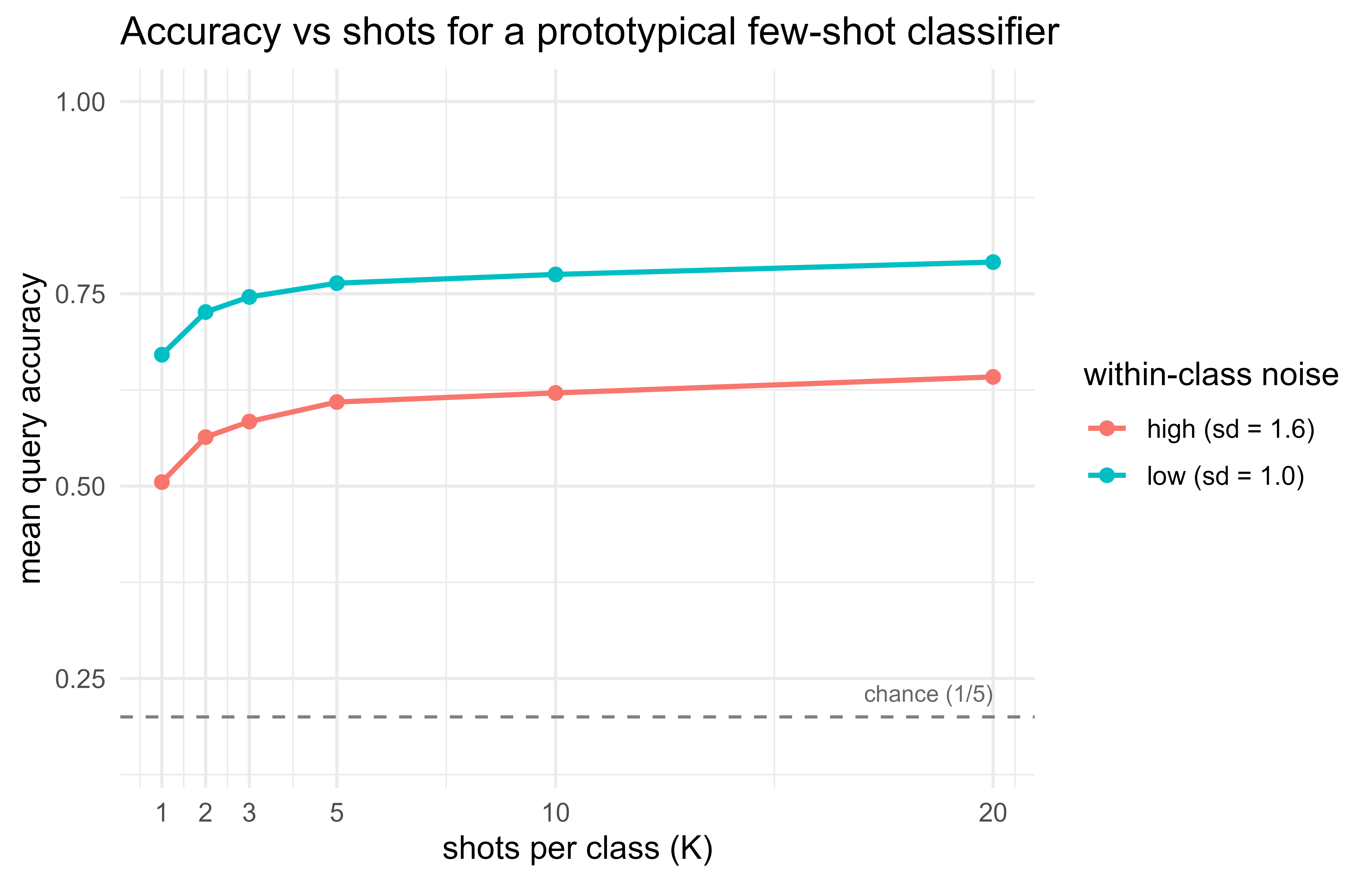
Figure 53.1 plots accuracy against the number of shots. The chance baseline for a 5-way task is \(1/5 = 0.2\).
Show code
library(ggplot2)plot_df<-rbind(data.frame(shots =shots, accuracy =acc_easy, noise ="low (sd = 1.0)"),data.frame(shots =shots, accuracy =acc_hard, noise ="high (sd = 1.6)"))ggplot(plot_df, aes(shots, accuracy, color =noise))+geom_hline(yintercept =0.2, linetype ="dashed", color ="grey50")+geom_line(linewidth =0.9)+geom_point(size =2)+annotate("text", x =max(shots), y =0.22, label ="chance (1/5)", hjust =1, vjust =0, size =3, color ="grey40")+scale_x_continuous(breaks =shots)+scale_y_continuous(limits =c(0.15, 1))+labs(x ="shots per class (K)", y ="mean query accuracy", color ="within-class noise", title ="Accuracy vs shots for a prototypical few-shot classifier")+theme_minimal(base_size =12)
Figure 53.1: Few-shot accuracy of a nearest-centroid (prototypical) classifier on simulated 5-way episodes. Accuracy rises with the number of shots K and saturates; higher within-class noise lowers the whole curve.
Two patterns are worth reading off the curve. First, even 1-shot accuracy is far above the chance line of \(0.2\), because a single support point already locates each blob roughly. Second, the gain from \(K=1\) to \(K=5\) is large and then flattens, which is the \(1/K\) variance reduction of the prototype estimate in action. Raising the noise shifts the whole curve down because the classes overlap more, so no amount of averaging fully separates them.
53.5.1 Why accuracy rises and saturates: the \(1/K\) law
The shape of the curve follows from a short calculation. Take the demo’s generative model: class \(c\) has true center \(\mu_c\) and support points \(x \sim \mathcal{N}(\mu_c, \sigma^2 I_p)\) drawn independently. The prototype is the sample mean of \(K\) such points,
So the prototype is an unbiased estimate of the class center whose error covariance shrinks like \(1/K\). Consider the two-class subproblem \(c\) versus \(c'\) with separation \(\Delta = \lVert \mu_c - \mu_{c'}\rVert\). A query from class \(c\) is \(x^\* = \mu_c + \eta\), \(\eta\sim\mathcal{N}(0,\sigma^2 I_p)\), and the nearest-centroid rule assigns it to \(c\) when it is closer to \(\mathbf{p}_c\) than to \(\mathbf{p}_{c'}\). Projecting onto the prototype-difference direction, a standard LDA-style calculation gives, in the limit \(K\to\infty\) where prototypes equal true centers, an error probability
with \(\Phi\) the standard normal CDF. For finite \(K\), the prototype noise adds to the query noise. Because \(\mathbf{p}_c\) and \(x^\*\) are independent, their contributions along the decision direction add in variance, inflating the effective noise from \(\sigma^2\) to \(\sigma^2\,(1 + 1/K)\) for the query-versus-one-prototype comparison (one factor \(\sigma^2\) from the query, one factor \(\sigma^2/K\) from the prototype). The Bayes-style two-class error becomes approximately
This reproduces both features of the plot. As \(K\to\infty\) the \(1/K\) term vanishes and the error saturates at the irreducible \(\Phi(-\Delta/2\sigma)\), the error of a classifier that knows the true centers; the residual gap at large \(K\) is set entirely by class overlap \(\Delta/\sigma\), not by the number of shots. The marginal gain from one more shot is the derivative of Equation 53.6 in \(1/K\), which is largest at small \(K\) and decays, matching the steep-then-flat curve. Raising \(\sigma\) lowers \(\Delta/\sigma\) and shifts the whole curve down, exactly as the high-noise line shows. Note the sample-complexity reading: to halve the excess error over the irreducible floor you need to drive \(1/K\) down, so returns diminish quadratically fast, and there is little reason to collect many shots once \(K\) is around \(5\) to \(10\) for well-separated classes.
Show code
# Verify the 1/K shrinkage of prototype variance (eq-meta-learning.qmd-proto-var).set.seed(1301)sigma<-1.3; p<-4; reps<-4000emp_var<-function(K){# Monte Carlo variance of one coordinate of the K-point sample mean.means<-replicate(reps, mean(rnorm(K, sd =sigma)))var(means)}Ks<-c(1, 2, 5, 10, 20)data.frame( K =Ks, empirical =round(sapply(Ks, emp_var), 4), theory_1_K =round(sigma^2/Ks, 4))#> K empirical theory_1_K#> 1 1 1.6271 1.6900#> 2 2 0.8689 0.8450#> 3 5 0.3422 0.3380#> 4 10 0.1696 0.1690#> 5 20 0.0852 0.0845
The empirical per-coordinate variance of the prototype tracks \(\sigma^2/K\) to Monte Carlo error, confirming Equation 53.5 that drives the accuracy curve.
53.5.2 A sketch of an encoder-based prototypical network (not run)
The demo above used the identity encoder. In practice the win comes from a learned encoder \(f_\theta\) trained episodically so that distances in embedding space respect class structure. The following Keras sketch shows the shape of that training loop. It is left unevaluated because it is illustrative pseudocode for the episodic loss rather than a packaged model.
Show code
library(keras)# f_theta: a small embedding network mapping inputs to R^d.make_encoder<-function(input_dim, embed_dim=16){keras_model_sequential()|>layer_dense(64, activation ="relu", input_shape =input_dim)|>layer_dense(embed_dim)}# One episode's prototypical loss: embed support and query, form prototypes,# score queries by negative squared distance, take softmax cross-entropy.proto_loss<-function(encoder, support_x, support_y, query_x, query_y,n_way){z_s<-encoder(support_x)# (N*K, d)z_q<-encoder(query_x)# (Nq, d)protos<-tf$stack(lapply(seq_len(n_way)-1L, function(c){mask<-tf$equal(support_y, c)tf$reduce_mean(tf$boolean_mask(z_s, mask), axis =0L)}))# (N, d)# pairwise squared distances query-to-prototyped2<-tf$reduce_sum((tf$expand_dims(z_q, 1L)-tf$expand_dims(protos, 0L))^2, axis =2L)logits<--d2tf$reduce_mean(tf$nn$sparse_softmax_cross_entropy_with_logits( labels =query_y, logits =logits))}# Meta-training: sample episodes, accumulate gradients of proto_loss# through the encoder, and step an optimizer. Each step is one episode.
The base-R demo and this sketch share the same prediction rule. The only difference is whether the feature map is fixed (identity) or trained end to end through the episodic loss.
Tip
When you move from this toy to a real prototypical network, the identity encoder is replaced by make_encoder, but the loss, the prototypes, and the nearest-prototype decision rule stay exactly as written here. Read the base-R proto_predict and the Keras proto_loss side by side: they compute the same thing.
53.6 Practical guidance, pitfalls, and when to use
The methods above are appealing, but the decision to use meta-learning at all is the one that matters most in practice. The single most common mistake is reaching for a meta-learner when a simpler tool would do better, so we start there.
When to use this
Meta-learning earns its complexity only when two conditions hold at once: you face a stream of related tasks, and each new task gives you very few labels. If either condition fails, a standard model or a fine-tuned pretrained model is usually the better and simpler choice.
When to reach for meta-learning.
You face a stream of new tasks that resemble each other, and each new task has only a few labels (single digits to low tens per class).
You can assemble a meta-training set of many tasks drawn from a distribution close to deployment tasks. This last condition is the one people most often violate.
When not to.
You have one fixed task with plenty of labels. Train a standard model.
You have one task with few labels but a large related labeled corpus. Fine-tuning a pretrained model is usually simpler and stronger than building a meta-learner.
Your deployment tasks are not exchangeable with your meta-training tasks. Meta-learning generalizes across tasks only to the extent that train and test tasks come from the same \(p(\mathcal{T})\).
Pitfalls.
Task leakage and overlapping classes. If the same classes appear in meta-training and meta-test, reported few-shot accuracy is inflated. Split by class, not just by example.
Episode composition matters. Reported numbers depend on \(N\), \(K\), the query size, and how episodes are sampled. Always state the \(N\)-way \(K\)-shot configuration, and average over many episodes with confidence intervals, since per-episode accuracy is noisy.
Choose the family by your deployment budget. Metric-based methods (prototypical, matching) need no per-task gradient step, so they are cheap and robust to serve. Optimization-based methods (MAML) are more flexible but require an inner adaptation loop and careful tuning of the inner learning rate and step count.
Distance metric and feature scale. Prototypical networks assume distances are meaningful. Unnormalized or differently scaled features distort Euclidean distances; standardize features or learn an embedding that does so.
Class imbalance within a task (Chapter 80). Prototypes from very few points are high variance. With \(K=1\) a single outlier support point can dislocate a whole class prototype.
Sanity checks. Compare against a nearest-centroid baseline on raw or pretrained features (exactly the demo above). A learned meta-learner that does not beat this simple baseline is not earning its complexity. Also report the chance level \(1/N\) so improvements are interpretable.
Warning
The most damaging error in few-shot work is silent: if a class appears in both meta-training and meta-test, the model has effectively already seen the answer, and reported accuracy is meaningless. Always split by class, not just by example, and state the exact \(N\)-way \(K\)-shot configuration alongside every number.
To summarize the chapter: meta-learning trades an expensive offline phase, training across many tasks under the episodic protocol, for cheap adaptation to new tasks from a few labels. Optimization-based methods like MAML adapt by taking gradient steps from a learned initialization, while metric-based methods like prototypical and matching networks adapt by comparing query points to a learned representation of the support set. The runnable demo showed the engine inside the metric-based family in its simplest form: averaging support points to form class prototypes, where accuracy climbs with the number of shots and then saturates as the \(1/K\) variance reduction runs out. When you decide whether to use any of this, let the two questions in the callout above, “are the tasks related?” and “are labels truly scarce?”, make the call.
53.7 Further reading
Vinyals, Blundell, Lillicrap, Kavukcuoglu, and Wierstra (2016). “Matching Networks for One Shot Learning.”
Finn, Abbeel, and Levine (2017). “Model-Agnostic Meta-Learning for Fast Adaptation of Deep Networks” (MAML).
Snell, Swersky, and Zemel (2017). “Prototypical Networks for Few-shot Learning.”
Nichol, Achiam, and Schulman (2018). “On First-Order Meta-Learning Algorithms” (Reptile).
Ravi and Larochelle (2017). “Optimization as a Model for Few-Shot Learning.”
Hospedales, Antoniou, Micaelli, and Storkey (2021). “Meta-Learning in Neural Networks: A Survey.”
Wang, Yao, Kwok, and Ni (2020). “Generalizing from a Few Examples: A Survey on Few-Shot Learning.”
The vocabulary is borrowed from card games and learning theory: a “shot” is one labeled example you are allowed to see per class, and “\(N\)-way” counts how many classes the model must choose among. A 5-way 1-shot task is therefore a five-class problem with a single labeled example per class.↩︎
The prototype \(\mathbf{p}_c\) is just the centroid (average position) of class \(c\)’s support embeddings. Classifying a query by its nearest prototype is the centuries-old nearest-centroid rule, lifted into a learned feature space.↩︎
Source Code
# Meta-Learning and Few-Shot Learning {#sec-meta-learning}```{r}#| include: falsesource("_common.R")```Most supervised methods in this book assume access to a large labeled training set for one fixed task. Meta-learning relaxes that assumption. The goal is to build a system that can adapt to a *new* task from only a handful of labeled examples, by reusing structure learned across many *related* tasks. The slogan is "learning to learn": rather than learning a single predictor, we learn a procedure that produces good predictors quickly.This chapter covers the conceptual core of meta-learning (optimization-based methods such as MAML and metric-based methods such as prototypical and matching networks), the episodic training protocol, and the $N$-way $K$-shot evaluation setup. The runnable demonstration is a nearest-centroid (prototypical) few-shot classifier implemented in base R, evaluated on simulated episodes, where we measure how accuracy improves as the number of shots per class grows.::: {.callout-tip title="Intuition"}A standard model learns *what the answer is* for one task. A meta-learner learns *how to find the answer* for a whole family of tasks, so that when a brand new task arrives with only a few labels, it already knows where to look. Think of the difference between memorizing one map and learning to read maps in general.:::## Where this fits in a modern ML workflowIn a typical applied setting you train once on a large dataset and serve that model. Few-shot learning targets a different operating regime:- A new product category appears with only 5 labeled images per class.- A fraud pattern emerges and you have 10 confirmed cases.- A clinical phenotype is rare, so per-patient labels are scarce.Collecting thousands of labels per new task is slow or impossible. Meta-learning amortizes that cost: you pay an expensive offline phase on many tasks that resemble the deployment tasks, and in return you get cheap, fast adaptation at deployment. In modern AI pipelines this idea sits next to two cousins that practitioners often confuse with it:- Transfer learning / fine-tuning (@sec-transfer-multitask-learning). Pretrain a large model, then fine-tune on the new task. This usually needs more than a handful of labels and a gradient-descent run per task.- In-context learning with large language models (@sec-llms). The model conditions on a few examples in its prompt and adapts with no weight update. This is, in effect, meta-learning whose "training across tasks" happened implicitly during pretraining.Few-shot meta-learning is the explicit, supervised version of the same objective: optimize directly for fast adaptation from few examples.::: {.callout-important title="Key idea"}The cost of learning a new task is not eliminated, it is moved. Meta-learning pays a heavy bill once, offline, by training across many tasks, and is repaid with cheap, fast adaptation every time a new task arrives.:::### Notation and the task distributionWe assume a distribution over tasks $p(\mathcal{T})$. A task $\mathcal{T}_i$ is itself a small learning problem with its own data. For classification, each task draws $N$ classes and provides:- a support set $\mathcal{S} = \{(x_j, y_j)\}_{j=1}^{N K}$ with $K$ labeled examples per class (so $N K$ examples total),- a query set $\mathcal{Q} = \{(x_j^\*, y_j^\*)\}$ used to score how well the model adapted using $\mathcal{S}$.This is the $N$-way $K$-shot setup: $N$ classes, $K$ labeled examples each.^[The vocabulary is borrowed from card games and learning theory: a "shot" is one labeled example you are allowed to see per class, and "$N$-way" counts how many classes the model must choose among. A 5-way 1-shot task is therefore a five-class problem with a single labeled example per class.] A "5-way 1-shot" task means five classes with a single labeled example per class. The important constraint is that the classes (and often the entire label space) differ between tasks. A model that simply memorizes a fixed set of categories cannot solve held-out tasks; it must learn a transferable adaptation rule.::: {.callout-note}The split into support and query within a single task is what makes meta-learning more than a renaming of supervised learning. The support set plays the role of "training data the model is allowed to adapt on" and the query set plays the role of "test data," but both live *inside* one task, and we repeat this train/test split thousands of times across tasks.:::## Episodic trainingThe training signal mirrors the test condition. Instead of iterating over mini-batches of individual examples, we iterate over episodes, where each episode is a sampled task $(\mathcal{S}, \mathcal{Q})$. The meta-objective averages the query loss after adaptation on the support set:$$\min_{\theta}\; \mathbb{E}_{\mathcal{T}_i \sim p(\mathcal{T})}\;\big[\, \mathcal{L}_{\mathcal{Q}_i}\big( A(\theta, \mathcal{S}_i) \big) \,\big],$$where $\theta$ are the meta-parameters, $A(\theta, \mathcal{S})$ is the adaptation procedure that turns $\theta$ and a support set into a task-specific predictor, and $\mathcal{L}_{\mathcal{Q}}$ is the loss on the query set. Different meta-learning families differ mainly in what $A$ is.The reason episodic training works is that we never let the model see the query labels during adaptation; we only score on them. The gradient through that score teaches $\theta$ to make adaptation generalize, not to memorize.### The meta-objective as a bilevel programIt is worth stating the meta-objective precisely, because every family in this chapter is an instance of the same two-level (bilevel) optimization. Write the population meta-risk as$$\mathcal{R}(\theta) = \mathbb{E}_{\mathcal{T}_i \sim p(\mathcal{T})}\,\mathbb{E}_{(\mathcal{S}_i,\mathcal{Q}_i)}\,\big[\, \mathcal{L}_{\mathcal{Q}_i}\big(A(\theta,\mathcal{S}_i)\big)\,\big],$$ {#eq-meta-learning-bilevel}with the inner level defining the adapted predictor. For MAML the inner level is itself an optimization, $A(\theta,\mathcal{S}) = \arg\min_{\phi} \mathcal{L}_{\mathcal{S}}(\phi)$ approximated by a few gradient steps from $\phi^{(0)}=\theta$; for metric methods the inner level is a closed-form map (compute prototypes), so $A$ is differentiable in $\theta$ with no implicit dependence to unroll. In practice we minimize the empirical counterpart of @eq-meta-learning-bilevel over a finite sample of $B$ episodes,$$\widehat{\mathcal{R}}(\theta) = \frac{1}{B}\sum_{i=1}^{B} \mathcal{L}_{\mathcal{Q}_i}\big(A(\theta,\mathcal{S}_i)\big).$$Two distinct sources of variance enter $\widehat{\mathcal{R}}$: the sampling of tasks $\mathcal{T}_i$ and, within each task, the sampling of the support and query sets. The generalization quantity of interest is the gap between performance on meta-training tasks and on tasks freshly drawn from $p(\mathcal{T})$. This is a generalization bound over a *task distribution*, not over examples, which is why class-disjoint splits (discussed later) are essential: reusing classes makes the empirical $\widehat{\mathcal{R}}$ an optimistic estimate of $\mathcal{R}$.::: {.callout-note}The bilevel view also clarifies the difference from ordinary multi-task learning. Multi-task learning minimizes $\sum_i \mathcal{L}_i(\theta)$ over a *shared* $\theta$ with no inner adaptation, so it seeks one parameter good for all tasks on average. Meta-learning inserts the adaptation map $A$ inside the loss, so it seeks a $\theta$ that is good *after* adapting, which is a strictly weaker and usually easier requirement.:::::: {.callout-tip title="Intuition"}Train the way you will be tested. If deployment means "adapt from a handful of labels, then predict on new points," then every training episode should rehearse exactly that, adapt on a support set, predict on a held-out query set. The meta-objective rewards adaptation rules that transfer.:::With the training protocol in place, the families of methods differ only in the choice of the adaptation procedure $A$. We look at two: one that adapts by taking gradient steps, and one that adapts by comparing distances.## Optimization-based meta-learning: MAML (conceptual)Model-Agnostic Meta-Learning (Finn, Abbeel, and Levine, 2017) chooses $A$ to be a few steps of gradient descent. The meta-parameters $\theta$ are an *initialization*. For a task with support set $\mathcal{S}_i$, the adapted parameters after one inner step are$$\theta_i' = \theta - \alpha \nabla_{\theta}\, \mathcal{L}_{\mathcal{S}_i}(\theta),$$with inner step size $\alpha$. The outer (meta) objective evaluates these adapted parameters on the query set and updates the initialization:$$\theta \leftarrow \theta - \beta \,\nabla_{\theta} \sum_{i} \mathcal{L}_{\mathcal{Q}_i}(\theta_i').$$Because $\theta_i'$ already depends on $\theta$, the outer gradient differentiates through the inner update, producing a second-order term involving the Hessian $\nabla^2_\theta \mathcal{L}_{\mathcal{S}_i}(\theta)$. Expanding the chain rule for one inner step,$$\nabla_{\theta}\, \mathcal{L}_{\mathcal{Q}_i}(\theta_i')= \big( I - \alpha\, \nabla^2_{\theta}\, \mathcal{L}_{\mathcal{S}_i}(\theta) \big)\,\nabla_{\theta'} \mathcal{L}_{\mathcal{Q}_i}(\theta_i').$$The intuition: MAML does not look for parameters that are good on any single task. It looks for an initialization from which a *short* gradient run lands on a good task-specific solution. First-order variants (FOMAML, Reptile from Nichol, Achiam, and Schulman, 2018) drop the Hessian term and work well in practice at lower cost.### Derivation of the meta-gradientThe expansion above is worth deriving carefully, because the Hessian term is the entire content of "second-order MAML." Fix a task $i$ and define the inner map $\theta_i'(\theta) = \theta - \alpha \nabla_\theta \mathcal{L}_{\mathcal{S}_i}(\theta)$. Its Jacobian with respect to $\theta$ is, entry by entry,$$\frac{\partial \theta_i'}{\partial \theta}= I - \alpha\, \nabla^2_\theta \mathcal{L}_{\mathcal{S}_i}(\theta),$$ {#eq-meta-learning-inner-jac}a symmetric $d \times d$ matrix, where $d = \dim(\theta)$ and $\nabla^2_\theta \mathcal{L}_{\mathcal{S}_i}$ is the Hessian of the support loss. By the chain rule, the meta-gradient of the per-task query loss is the Jacobian transpose times the query gradient evaluated at the adapted point,$$\nabla_\theta\, \mathcal{L}_{\mathcal{Q}_i}\big(\theta_i'(\theta)\big)= \Big(\frac{\partial \theta_i'}{\partial \theta}\Big)^{\!\top}\,\nabla_{\theta'} \mathcal{L}_{\mathcal{Q}_i}(\theta_i')= \big(I - \alpha\, \nabla^2_\theta \mathcal{L}_{\mathcal{S}_i}(\theta)\big)\,\nabla_{\theta'} \mathcal{L}_{\mathcal{Q}_i}(\theta_i'),$$ {#eq-meta-learning-maml-grad}which is exactly the displayed result (the Hessian is symmetric so the transpose drops out). Reading @eq-meta-learning-maml-grad term by term: the $I$ piece is the naive "pretend the init does not move" gradient, and the $-\alpha \nabla^2 \mathcal{L}_{\mathcal{S}_i}$ piece is the correction that accounts for how perturbing $\theta$ changes where one inner step lands. FOMAML simply sets the second term to zero, using $\nabla_\theta \mathcal{L}_{\mathcal{Q}_i}(\theta_i') \approx \nabla_{\theta'} \mathcal{L}_{\mathcal{Q}_i}(\theta_i')$, which is the gradient of the query loss evaluated at $\theta_i'$ but treated as if $\theta_i'$ were a constant.For $m$ inner steps with iterates $\theta^{(0)}=\theta,\, \theta^{(t+1)} = \theta^{(t)} - \alpha \nabla \mathcal{L}_{\mathcal{S}_i}(\theta^{(t)})$, the Jacobian chains multiplicatively:$$\frac{\partial \theta^{(m)}}{\partial \theta}= \prod_{t=0}^{m-1}\big(I - \alpha\, \nabla^2_\theta \mathcal{L}_{\mathcal{S}_i}(\theta^{(t)})\big),$$so the exact meta-gradient is a product of $m$ Hessian-perturbed factors applied to $\nabla_{\theta^{(m)}} \mathcal{L}_{\mathcal{Q}_i}$. Materializing these $d \times d$ factors is infeasible for large $d$; instead, reverse-mode automatic differentiation computes the required Hessian-vector products $\nabla^2 \mathcal{L}_{\mathcal{S}_i}\, v$ in $O(d)$ time each (Pearlmutter's trick), giving the meta-gradient in time and memory $O(md)$, the memory cost coming from storing the $m$ intermediate activations needed for the backward pass.### Reptile and why first-order worksReptile dispenses with the support/query split inside a task: it runs $m$ steps of ordinary SGD on a task to reach $\theta^{(m)}$, then moves the meta-parameters toward that point, $\theta \leftarrow \theta + \epsilon\,(\theta^{(m)} - \theta)$. To see why this approximates MAML, Taylor-expand the per-step gradients around $\theta$. For two steps, writing $g_t = \nabla \mathcal{L}_t(\theta)$ and $H_t = \nabla^2 \mathcal{L}_t(\theta)$ for the loss on the $t$-th minibatch, the expected Reptile update direction is$$\mathbb{E}\big[\theta^{(m)} - \theta\big]= -\alpha\sum_t \mathbb{E}[g_t]+ \alpha^2 \sum_{t < t'} \mathbb{E}[H_{t'} g_t] + O(\alpha^3).$$The leading term is joint minimization of the average task loss (ordinary multi-task pretraining), while the second term $\mathbb{E}[H_{t'} g_t]$ is an inner product between gradients of different minibatches of the *same* task. Maximizing that cross term pushes the gradients of distinct batches to align, which is precisely the quantity MAML's Hessian term optimizes: an initialization where within-task gradients agree generalizes from few examples. This is why dropping the explicit second-order term costs little. The expensive Hessian is recovered, in expectation, by the interaction of successive first-order steps.MAML is "model-agnostic" because $A$ is just gradient descent, so it applies to any differentiable model. The price is the inner loop: each meta-update requires adapting and backpropagating through adaptation, which is memory-hungry and sensitive to the inner step count and learning rate.::: {.callout-warning}Differentiating through the inner gradient step is what produces the Hessian term above, and it is the main source of MAML's fragility and cost. If MAML is unstable or too slow, the first thing to try is a first-order variant (FOMAML or Reptile), which drops that second-order term.:::Optimization-based methods adapt by *moving the weights*. The next family adapts without touching the weights at all.## Metric-based meta-learningMetric-based methods skip the inner gradient loop. The adaptation procedure $A$ embeds inputs into a feature space with a learned encoder $f_\theta$, then classifies query points by comparison to the support set. There is no per-task weight update at deployment, only a distance computation, which makes these methods fast and stable.### Prototypical networksPrototypical networks (Snell, Swersky, and Zemel, 2017) represent each class by the mean of its support embeddings (its prototype). For class $c$ with support subset $\mathcal{S}_c$,$$\mathbf{p}_c = \frac{1}{|\mathcal{S}_c|} \sum_{(x,y)\in \mathcal{S}_c} f_\theta(x).$$A query point $x^\*$ is classified by its squared Euclidean distance to each prototype,^[The prototype $\mathbf{p}_c$ is just the centroid (average position) of class $c$'s support embeddings. Classifying a query by its nearest prototype is the centuries-old nearest-centroid rule, lifted into a learned feature space.] turned into a softmax over classes:$$P(y^\* = c \mid x^\*) =\frac{\exp\!\big(-\, d(f_\theta(x^\*), \mathbf{p}_c)\big)}{\sum_{c'} \exp\!\big(-\, d(f_\theta(x^\*), \mathbf{p}_{c'})\big)},\qquadd(u, v) = \lVert u - v \rVert_2^2 .$$Training minimizes the negative log probability of the true class on query points, averaged over episodes. A clean fact: with squared Euclidean distance, the prototype rule is a linear classifier in embedding space, since expanding $-\lVert u - \mathbf{p}_c \rVert^2$ gives a term linear in $u$ plus a per-class bias. This is why nearest-centroid classification is the natural base-R stand-in for a prototypical network with a fixed (or identity) encoder.#### Derivation: prototypes give a linear classifierLet $u = f_\theta(x^\*)$ be the query embedding. Expand the negative squared distance that forms the logit for class $c$:$$-\lVert u - \mathbf{p}_c \rVert_2^2= -u^\top u + 2\,\mathbf{p}_c^\top u - \mathbf{p}_c^\top \mathbf{p}_c .$$The term $-u^\top u$ does not depend on $c$, so it cancels in the softmax (and in any argmax over classes). Discarding it leaves a logit that is affine in $u$,$$\ell_c(u) = w_c^\top u + b_c,\qquadw_c = 2\,\mathbf{p}_c,\qquadb_c = -\,\mathbf{p}_c^\top \mathbf{p}_c = -\lVert \mathbf{p}_c\rVert_2^2 .$$ {#eq-meta-learning-proto-linear}Hence $P(y^\*=c\mid x^\*) = \mathrm{softmax}_c(\ell_c(u))$ is exactly a linear softmax (multinomial logistic) classifier whose weight vectors and biases are *tied to the prototypes* rather than learned freely. The decision boundary between classes $c$ and $c'$ is the locus $\ell_c(u) = \ell_{c'}(u)$, i.e. $2(\mathbf{p}_c - \mathbf{p}_{c'})^\top u = \lVert \mathbf{p}_c\rVert^2 - \lVert \mathbf{p}_{c'}\rVert^2$, which is the perpendicular bisector hyperplane of the segment joining the two prototypes. This is the classical nearest-centroid (and, under equal isotropic covariances, linear discriminant) geometry, now living in the learned embedding space.#### Connection to Gaussian generative classificationThe squared-Euclidean choice is not arbitrary. Suppose that, in embedding space, class $c$ is Gaussian with mean $\mathbf{p}_c$ and shared isotropic covariance $\sigma^2 I$, and classes are equally likely a priori. The class posterior is$$P(c\mid u) \propto \exp\!\Big(-\tfrac{1}{2\sigma^2}\lVert u - \mathbf{p}_c\rVert^2\Big),$$which is exactly the prototypical softmax with logits scaled by $1/(2\sigma^2)$. Snell, Swersky, and Zemel (2017) make this precise: with squared Euclidean distance the prototypical network is performing linear discriminant analysis in feature space, and more generally it is a Bregman-divergence centroid classifier. For any regular Bregman divergence $d_\varphi$, the cluster representative that minimizes mean within-class divergence is the arithmetic mean, $\mathbf{p}_c = \tfrac{1}{|\mathcal{S}_c|}\sum_{x\in\mathcal{S}_c} f_\theta(x)$, which is why the *mean* is the correct prototype. Squared Euclidean distance is the Bregman divergence generated by $\varphi(z)=\lVert z\rVert^2$. This also explains a common empirical finding: cosine distance often underperforms squared Euclidean for prototypical networks precisely because cosine is not a Bregman divergence, so the support mean is no longer the divergence-optimal representative.::: {.callout-note}The Bregman view tells you when averaging support embeddings is the right thing to do. If your distance is squared Euclidean (or any Bregman divergence), the prototype should be the mean. If you switch to cosine or another non-Bregman metric, the mean is no longer optimal and you may need a different aggregation (for example $\ell_2$-normalizing embeddings first, which makes squared Euclidean and cosine agree up to a constant).:::### Matching networksMatching networks (Vinyals et al., 2016) predict by a weighted vote over support labels, where the weights are an attention kernel (see @sec-transformers) between the query and each support embedding:$$\hat{y}^\* = \sum_{(x_j, y_j) \in \mathcal{S}} a(x^\*, x_j)\, \mathbf{1}[y_j = c],\qquada(x^\*, x_j) = \frac{\exp\!\big(\cos(f_\theta(x^\*), g_\theta(x_j))\big)}{\sum_{k} \exp\!\big(\cos(f_\theta(x^\*), g_\theta(x_k))\big)}.$$Here the prediction $\hat y^\*$ is read as the vector of class scores: stacking the indicators $\mathbf{1}[y_j=c]$ over classes, the matching-network output is $P(y^\*=c\mid x^\*) = \sum_{j} a(x^\*,x_j)\,\mathbf{1}[y_j=c]$, a convex combination of one-hot support labels with attention weights $a(x^\*,x_j)\ge 0$ summing to one. This is exactly a Nadaraya-Watson kernel estimator (@sec-kernel) with a softmax-of-cosine kernel: the prediction is a kernel-weighted average of support labels, learned end to end through the embedding $f_\theta$, $g_\theta$. Viewed this way, matching networks are nonparametric (their effective model grows with the support set), whereas prototypical networks compress the support into $N$ parametric prototypes before predicting.When $K = 1$, prototypical and matching networks coincide up to the choice of distance (squared Euclidean versus cosine), because each prototype is just the single support point. For $K > 1$, prototypes average within a class while matching networks keep every support point as a separate voter. The bias-variance trade-off between them is the usual parametric-versus-nonparametric one: prototypes lower variance by averaging (good when within-class clusters are unimodal and roughly isotropic, as the Gaussian model above assumes) but incur bias if a class is multimodal, in which case the per-point voting of matching networks, which can represent several modes per class, is less biased at the cost of higher variance from individual noisy support points.### Comparison of the main families@tbl-meta-learning-family-comparison contrasts the main meta-learning families along the axes that matter most when choosing one: how each adapts at test time, whether it updates weights per task, its deployment cost, and what it is sensitive to.| Family | Adaptation $A$ at test time | Per-task weight update | Compute at deployment | Sensitive to | Representative work ||---|---|---|---|---|---|| Optimization-based (MAML, Reptile) | Few gradient steps from a learned init | Yes | High (inner loop, second-order) | Inner LR, step count | Finn et al. 2017; Nichol et al. 2018 || Prototypical networks | Compute class means, nearest prototype | No | Low (distance to $N$ prototypes) | Embedding quality, distance metric | Snell et al. 2017 || Matching networks | Attention-weighted vote over support | No | Low to medium ($NK$ comparisons) | Embedding quality, kernel | Vinyals et al. 2016 || Fine-tuning a pretrained model | Standard supervised training | Yes | Medium to high | Needs more labels than few-shot | Transfer learning, broadly |: Comparison of the main meta-learning families by adaptation rule, whether weights update per task, deployment compute, key sensitivities, and representative work. {#tbl-meta-learning-family-comparison}## Runnable demo: nearest-centroid few-shot classifierWe implement the prototypical idea with the simplest possible encoder, the identity map, so the "embedding" is the raw feature vector. We simulate a task distribution where each class is a Gaussian blob with a random center, draw episodes, and classify query points by nearest class centroid (the prototype). We then measure query accuracy as a function of the number of shots $K$.This isolates the mechanism that prototypical networks rely on: averaging $K$ support points reduces the variance of the prototype estimate, which moves the decision boundary closer to the Bayes-optimal one and raises accuracy. With $K$ independent support points per class, the prototype is the sample mean, whose variance shrinks like $1/K$, so accuracy should rise and then saturate.::: {.callout-important title="Key idea"}More shots help because each extra labeled example sharpens the estimate of the class center, not because the model "learns more." The $1/K$ variance reduction of an average is the whole story behind the rising accuracy curve we are about to plot.:::```{r proto-setup, eval=TRUE}set.seed(1301)# Sample one N-way K-shot episode from a Gaussian task distribution.# Each class is a blob with a random center in p dimensions and shared sd.sample_episode <-function(n_way, k_shot, n_query, p =2, sd =1.0,center_spread =2.5) { centers <-matrix(rnorm(n_way * p, sd = center_spread), nrow = n_way) draw <-function(n_per_class) { X <-matrix(0, nrow = n_way * n_per_class, ncol = p) y <-integer(n_way * n_per_class) row <-1Lfor (c inseq_len(n_way)) {for (j inseq_len(n_per_class)) { X[row, ] <- centers[c, ] +rnorm(p, sd = sd) y[row] <- c row <- row +1L } }list(X = X, y = y) }list(support =draw(k_shot), query =draw(n_query))}# Prototypical classifier with identity encoder: class prototypes are the# support means, queries go to the nearest prototype (squared Euclidean).proto_predict <-function(support, query_X, n_way) { p <-ncol(support$X) protos <-matrix(0, nrow = n_way, ncol = p)for (c inseq_len(n_way)) { protos[c, ] <-colMeans(support$X[support$y == c, , drop =FALSE]) }# squared Euclidean distance from each query point to each prototype d2 <-matrix(0, nrow =nrow(query_X), ncol = n_way)for (c inseq_len(n_way)) { diff <-sweep(query_X, 2, protos[c, ], "-") d2[, c] <-rowSums(diff^2) }max.col(-d2, ties.method ="first") # argmin distance = argmax negative dist}# Average query accuracy over many episodes for a given K.eval_shots <-function(k_shot, n_episodes =400, n_way =5,n_query =15, p =2, sd =1.0) { acc <-numeric(n_episodes)for (e inseq_len(n_episodes)) { ep <-sample_episode(n_way, k_shot, n_query, p = p, sd = sd) pred <-proto_predict(ep$support, ep$query$X, n_way) acc[e] <-mean(pred == ep$query$y) }mean(acc)}```Now we sweep the number of shots and record mean accuracy. We repeat the sweep at two noise levels to show how task difficulty interacts with the number of shots. @tbl-meta-learning-shot-accuracy reports the mean query accuracy at each shot count under both noise levels.```{r proto-sweep, eval=TRUE}shots <-c(1, 2, 3, 5, 10, 20)set.seed(7)acc_easy <-sapply(shots, eval_shots, n_episodes =400, n_way =5, sd =1.0)set.seed(7)acc_hard <-sapply(shots, eval_shots, n_episodes =400, n_way =5, sd =1.6)results <-data.frame(shots = shots,acc_low_noise =round(acc_easy, 3),acc_high_noise =round(acc_hard, 3))``````{r tbl-meta-learning-shot-accuracy, eval=TRUE}knitr::kable( results,caption ="Mean query accuracy of the nearest-centroid few-shot classifier on simulated 5-way episodes, by shots per class and within-class noise level, averaged over 400 episodes.",col.names =c("shots (K)", "accuracy (low noise)", "accuracy (high noise)"))```@fig-meta-learning-proto-figure plots accuracy against the number of shots. The chance baseline for a 5-way task is $1/5 = 0.2$.```{r fig-meta-learning-proto-figure, eval=TRUE, fig.cap="Few-shot accuracy of a nearest-centroid (prototypical) classifier on simulated 5-way episodes. Accuracy rises with the number of shots K and saturates; higher within-class noise lowers the whole curve.", fig.width=7, fig.height=4.5}library(ggplot2)plot_df <-rbind(data.frame(shots = shots, accuracy = acc_easy, noise ="low (sd = 1.0)"),data.frame(shots = shots, accuracy = acc_hard, noise ="high (sd = 1.6)"))ggplot(plot_df, aes(shots, accuracy, color = noise)) +geom_hline(yintercept =0.2, linetype ="dashed", color ="grey50") +geom_line(linewidth =0.9) +geom_point(size =2) +annotate("text", x =max(shots), y =0.22,label ="chance (1/5)", hjust =1, vjust =0, size =3,color ="grey40") +scale_x_continuous(breaks = shots) +scale_y_continuous(limits =c(0.15, 1)) +labs(x ="shots per class (K)", y ="mean query accuracy",color ="within-class noise",title ="Accuracy vs shots for a prototypical few-shot classifier") +theme_minimal(base_size =12)```Two patterns are worth reading off the curve. First, even 1-shot accuracy is far above the chance line of $0.2$, because a single support point already locates each blob roughly. Second, the gain from $K=1$ to $K=5$ is large and then flattens, which is the $1/K$ variance reduction of the prototype estimate in action. Raising the noise shifts the whole curve down because the classes overlap more, so no amount of averaging fully separates them.### Why accuracy rises and saturates: the $1/K$ lawThe shape of the curve follows from a short calculation. Take the demo's generative model: class $c$ has true center $\mu_c$ and support points $x \sim \mathcal{N}(\mu_c, \sigma^2 I_p)$ drawn independently. The prototype is the sample mean of $K$ such points,$$\mathbf{p}_c = \frac{1}{K}\sum_{j=1}^{K} x_{c,j},\qquad\mathbb{E}[\mathbf{p}_c] = \mu_c,\qquad\mathrm{Cov}(\mathbf{p}_c) = \frac{\sigma^2}{K} I_p .$$ {#eq-meta-learning-proto-var}So the prototype is an unbiased estimate of the class center whose error covariance shrinks like $1/K$. Consider the two-class subproblem $c$ versus $c'$ with separation $\Delta = \lVert \mu_c - \mu_{c'}\rVert$. A query from class $c$ is $x^\* = \mu_c + \eta$, $\eta\sim\mathcal{N}(0,\sigma^2 I_p)$, and the nearest-centroid rule assigns it to $c$ when it is closer to $\mathbf{p}_c$ than to $\mathbf{p}_{c'}$. Projecting onto the prototype-difference direction, a standard LDA-style calculation gives, in the limit $K\to\infty$ where prototypes equal true centers, an error probability$$P(\text{misclassify}) = \Phi\!\Big(-\frac{\Delta}{2\sigma}\Big),$$with $\Phi$ the standard normal CDF. For finite $K$, the prototype noise adds to the query noise. Because $\mathbf{p}_c$ and $x^\*$ are independent, their contributions along the decision direction add in variance, inflating the effective noise from $\sigma^2$ to $\sigma^2\,(1 + 1/K)$ for the query-versus-one-prototype comparison (one factor $\sigma^2$ from the query, one factor $\sigma^2/K$ from the prototype). The Bayes-style two-class error becomes approximately$$P_K(\text{misclassify}) \approx \Phi\!\left(-\frac{\Delta}{2\sigma\sqrt{1 + 1/K}}\right).$$ {#eq-meta-learning-proto-err}This reproduces both features of the plot. As $K\to\infty$ the $1/K$ term vanishes and the error saturates at the irreducible $\Phi(-\Delta/2\sigma)$, the error of a classifier that knows the true centers; the residual gap at large $K$ is set entirely by class overlap $\Delta/\sigma$, not by the number of shots. The marginal gain from one more shot is the derivative of @eq-meta-learning-proto-err in $1/K$, which is largest at small $K$ and decays, matching the steep-then-flat curve. Raising $\sigma$ lowers $\Delta/\sigma$ and shifts the whole curve down, exactly as the high-noise line shows. Note the sample-complexity reading: to halve the *excess* error over the irreducible floor you need to drive $1/K$ down, so returns diminish quadratically fast, and there is little reason to collect many shots once $K$ is around $5$ to $10$ for well-separated classes.```{r proto-var-check, eval=TRUE}# Verify the 1/K shrinkage of prototype variance (eq-meta-learning.qmd-proto-var).set.seed(1301)sigma <-1.3; p <-4; reps <-4000emp_var <-function(K) {# Monte Carlo variance of one coordinate of the K-point sample mean. means <-replicate(reps, mean(rnorm(K, sd = sigma)))var(means)}Ks <-c(1, 2, 5, 10, 20)data.frame(K = Ks,empirical =round(sapply(Ks, emp_var), 4),theory_1_K =round(sigma^2/ Ks, 4))```The empirical per-coordinate variance of the prototype tracks $\sigma^2/K$ to Monte Carlo error, confirming @eq-meta-learning-proto-var that drives the accuracy curve.### A sketch of an encoder-based prototypical network (not run)The demo above used the identity encoder. In practice the win comes from a *learned* encoder $f_\theta$ trained episodically so that distances in embedding space respect class structure. The following Keras sketch shows the shape of that training loop. It is left unevaluated because it is illustrative pseudocode for the episodic loss rather than a packaged model.```{r proto-keras, eval=FALSE}library(keras)# f_theta: a small embedding network mapping inputs to R^d.make_encoder <-function(input_dim, embed_dim =16) {keras_model_sequential() |>layer_dense(64, activation ="relu", input_shape = input_dim) |>layer_dense(embed_dim)}# One episode's prototypical loss: embed support and query, form prototypes,# score queries by negative squared distance, take softmax cross-entropy.proto_loss <-function(encoder, support_x, support_y, query_x, query_y, n_way) { z_s <-encoder(support_x) # (N*K, d) z_q <-encoder(query_x) # (Nq, d) protos <- tf$stack(lapply(seq_len(n_way) -1L, function(c) { mask <- tf$equal(support_y, c) tf$reduce_mean(tf$boolean_mask(z_s, mask), axis =0L) })) # (N, d)# pairwise squared distances query-to-prototype d2 <- tf$reduce_sum((tf$expand_dims(z_q, 1L) - tf$expand_dims(protos, 0L))^2, axis =2L) logits <--d2 tf$reduce_mean( tf$nn$sparse_softmax_cross_entropy_with_logits(labels = query_y, logits = logits))}# Meta-training: sample episodes, accumulate gradients of proto_loss# through the encoder, and step an optimizer. Each step is one episode.```The base-R demo and this sketch share the same prediction rule. The only difference is whether the feature map is fixed (identity) or trained end to end through the episodic loss.::: {.callout-tip}When you move from this toy to a real prototypical network, the identity encoder is replaced by `make_encoder`, but the loss, the prototypes, and the nearest-prototype decision rule stay exactly as written here. Read the base-R `proto_predict` and the Keras `proto_loss` side by side: they compute the same thing.:::## Practical guidance, pitfalls, and when to useThe methods above are appealing, but the decision to use meta-learning at all is the one that matters most in practice. The single most common mistake is reaching for a meta-learner when a simpler tool would do better, so we start there.::: {.callout-tip title="When to use this"}Meta-learning earns its complexity only when two conditions hold at once: you face a *stream of related tasks*, and each new task gives you *very few labels*. If either condition fails, a standard model or a fine-tuned pretrained model is usually the better and simpler choice.:::When to reach for meta-learning.- You face a stream of new tasks that resemble each other, and each new task has only a few labels (single digits to low tens per class).- You can assemble a meta-training set of many tasks drawn from a distribution close to deployment tasks. This last condition is the one people most often violate.When not to.- You have one fixed task with plenty of labels. Train a standard model.- You have one task with few labels but a large related labeled corpus. Fine-tuning a pretrained model is usually simpler and stronger than building a meta-learner.- Your deployment tasks are not exchangeable with your meta-training tasks. Meta-learning generalizes across tasks only to the extent that train and test tasks come from the same $p(\mathcal{T})$.Pitfalls.- Task leakage and overlapping classes. If the same classes appear in meta-training and meta-test, reported few-shot accuracy is inflated. Split by *class*, not just by example.- Episode composition matters. Reported numbers depend on $N$, $K$, the query size, and how episodes are sampled. Always state the $N$-way $K$-shot configuration, and average over many episodes with confidence intervals, since per-episode accuracy is noisy.- Choose the family by your deployment budget. Metric-based methods (prototypical, matching) need no per-task gradient step, so they are cheap and robust to serve. Optimization-based methods (MAML) are more flexible but require an inner adaptation loop and careful tuning of the inner learning rate and step count.- Distance metric and feature scale. Prototypical networks assume distances are meaningful. Unnormalized or differently scaled features distort Euclidean distances; standardize features or learn an embedding that does so.- Class imbalance within a task (@sec-class-imbalance). Prototypes from very few points are high variance. With $K=1$ a single outlier support point can dislocate a whole class prototype.Sanity checks. Compare against a nearest-centroid baseline on raw or pretrained features (exactly the demo above). A learned meta-learner that does not beat this simple baseline is not earning its complexity. Also report the chance level $1/N$ so improvements are interpretable.::: {.callout-warning}The most damaging error in few-shot work is silent: if a class appears in both meta-training and meta-test, the model has effectively already seen the answer, and reported accuracy is meaningless. Always split by class, not just by example, and state the exact $N$-way $K$-shot configuration alongside every number.:::To summarize the chapter: meta-learning trades an expensive offline phase, training across many tasks under the episodic protocol, for cheap adaptation to new tasks from a few labels. Optimization-based methods like MAML adapt by taking gradient steps from a learned initialization, while metric-based methods like prototypical and matching networks adapt by comparing query points to a learned representation of the support set. The runnable demo showed the engine inside the metric-based family in its simplest form: averaging support points to form class prototypes, where accuracy climbs with the number of shots and then saturates as the $1/K$ variance reduction runs out. When you decide whether to use any of this, let the two questions in the callout above, "are the tasks related?" and "are labels truly scarce?", make the call.## Further reading- Vinyals, Blundell, Lillicrap, Kavukcuoglu, and Wierstra (2016). "Matching Networks for One Shot Learning."- Finn, Abbeel, and Levine (2017). "Model-Agnostic Meta-Learning for Fast Adaptation of Deep Networks" (MAML).- Snell, Swersky, and Zemel (2017). "Prototypical Networks for Few-shot Learning."- Nichol, Achiam, and Schulman (2018). "On First-Order Meta-Learning Algorithms" (Reptile).- Ravi and Larochelle (2017). "Optimization as a Model for Few-Shot Learning."- Hospedales, Antoniou, Micaelli, and Storkey (2021). "Meta-Learning in Neural Networks: A Survey."- Wang, Yao, Kwok, and Ni (2020). "Generalizing from a Few Examples: A Survey on Few-Shot Learning."