32 Density Estimation
Suppose someone hands you a column of numbers: the response times of a web service over a day, the heights of a sample of customers, the brightness of pixels in a batch of images. Before you fit any model, a natural first question is simply, “what does this data look like?” Not the mean, not the variance, but the whole shape: where the values pile up, whether there are one or several peaks, how heavy the tails are, which regions are essentially empty. That shape is the probability density \(p(x)\), and estimating it from a finite sample is the subject of this chapter.
Density estimation sits quietly underneath a surprising amount of data science. A model that knows \(p(x)\) can score a new point by how probable it is, which is the foundation of anomaly detection (Chapter 87): rare points live where \(p(x)\) is small. It can draw new samples that resemble the training data, which is generation. It can supply the likelihood that statistical inference and Bayesian methods are built on. And it gives the working analyst something more humble but just as valuable: an honest picture of a variable that no summary statistic can capture. A bimodal distribution and a wide unimodal one can share the same mean and standard deviation while telling completely different stories.
This chapter builds up the main tools in order of sophistication. We start with the humble histogram, expose its weaknesses, and fix them with kernel density estimation (KDE), where the central practical problem turns out to be choosing a bandwidth. We then move from these nonparametric methods, which let the data speak with few assumptions, to a parametric model, the Gaussian mixture, fitted with the expectation-maximization (EM) algorithm. Finally we sketch normalizing flows, the modern neural approach that scales density estimation to high dimensions. Throughout, \(p(x)\) is the unknown density we want, and \(\hat{p}(x)\) is our estimate of it.
This chapter connects closely to two others. The generative view of density (sampling from \(\hat{p}\), scoring likelihoods) is developed further in the generative models chapter (Chapter 42), where variational autoencoders, GANs, and diffusion models all turn out to be density estimators in disguise. The use of \(\hat{p}(x)\) to flag rare points underlies the anomaly and outlier detection chapter (Chapter 87).
32.1 What we are estimating, and why it is hard
We observe an independent and identically distributed sample \(x_1, x_2, \ldots, x_n\) drawn from an unknown distribution with density \(p(x)\) on \(\mathbb{R}^d\). The density is the function whose integral over any region gives the probability of landing there:
\[ \Pr(X \in A) \;=\; \int_A p(x)\, dx, \qquad p(x) \ge 0, \qquad \int_{\mathbb{R}^d} p(x)\, dx = 1. \]
Our goal is an estimate \(\hat{p}(x)\) that is close to \(p(x)\) everywhere. “Close” is usually measured by a global error such as the mean integrated squared error,
\[ \mathrm{MISE}(\hat{p}) \;=\; \mathbb{E}\!\left[ \int \bigl( \hat{p}(x) - p(x) \bigr)^2 dx \right], \]
which, like any squared-error criterion, decomposes into a bias term and a variance term. That decomposition is the recurring tension of the whole chapter: smooth estimates have low variance but high bias (they wash out real features), while wiggly estimates have low bias but high variance (they invent features that are just noise). Every method below exposes one knob, the bin width, the bandwidth, the number of mixture components, that controls exactly this trade-off.
Density estimation is genuinely harder than regression, and the reason is the curse of dimensionality. To estimate \(p(x)\) at a point you need samples near that point, and in high dimensions almost no two points are near each other. The volume of a neighborhood grows exponentially with the dimension \(d\), so the number of samples needed to fill space grows exponentially too. The best achievable error of a nonparametric estimator degrades from roughly \(n^{-2/5}\) in one dimension to \(n^{-2/(4+d)}\) in \(d\) dimensions, which becomes useless well before \(d\) reaches double digits.1
Density estimation always trades bias against variance, controlled by a single smoothing knob. Too little smoothing tracks noise; too much erases real structure. The art is choosing the knob, and most of this chapter is about how.
32.2 Histograms
The histogram is the oldest density estimator and still the first thing to reach for. Partition the line into bins of width \(h\), count how many of the \(n\) observations fall in each bin, and divide by \(n h\) so the total area is one. For a point \(x\) in a bin containing \(\nu\) observations,
\[ \hat{p}_{\text{hist}}(x) \;=\; \frac{\nu}{n\,h}. \]
The division by \(h\) is what turns a count into a density: it makes the area of each bar equal to the fraction of data it contains, so the bars integrate to one regardless of bin width.
The histogram has two flaws that motivate everything after it. First, it is discontinuous, a staircase, even though most real densities are smooth. Second, and less obviously, it depends on where the bins start, not only on their width. Shift the bin edges by half a bin and a bimodal-looking histogram can collapse to a single hump, or vice versa. The result is an estimate that depends on an arbitrary choice the analyst never meant to make.
The bin width \(h\) is the smoothing knob. Wide bins give a blocky, low-variance, high-bias picture; narrow bins give a spiky, high-variance, low-bias one. A common automatic choice is Scott’s rule, \(h = 3.49\,\hat{\sigma}\,n^{-1/3}\), which minimizes the asymptotic integrated squared error for roughly Gaussian data, where \(\hat{\sigma}\) is the sample standard deviation.
32.2.1 Bias, variance, and where Scott’s rule comes from
The histogram is worth analyzing carefully because it is the simplest setting in which the bias-variance machinery and the slow nonparametric rate appear explicitly, and the algebra previews the KDE analysis that follows. Fix a bin \(B = [x_0, x_0 + h)\) and let \(x\) lie in it. The bin count \(\nu = \sum_{i=1}^n \mathbf{1}\{x_i \in B\}\) is binomial with \(n\) trials and success probability \(p_B = \int_B p(u)\,du\), so \(\mathbb{E}[\nu] = n p_B\) and \(\operatorname{Var}(\nu) = n p_B(1 - p_B)\). With \(\hat{p}_{\text{hist}}(x) = \nu/(nh)\),
\[ \mathbb{E}[\hat{p}_{\text{hist}}(x)] = \frac{p_B}{h}, \qquad \operatorname{Var}\bigl(\hat{p}_{\text{hist}}(x)\bigr) = \frac{p_B(1 - p_B)}{n h^2}. \]
A first-order Taylor expansion of \(p\) about the bin center \(c = x_0 + h/2\) gives \(p_B = \int_B p(u)\,du = h\,p(c) + O(h^3)\), where the linear term integrates to zero by symmetry about \(c\). Hence \(\mathbb{E}[\hat{p}_{\text{hist}}(x)] = p(c) + O(h^2)\), and expanding \(p(x)\) around \(c\) as well yields the leading bias at an interior point \(x\),
\[ \operatorname{Bias}\bigl(\hat{p}_{\text{hist}}(x)\bigr) \;\approx\; \Bigl(c - x\Bigr) p'(x), \qquad c - x \in \bigl[-\tfrac{h}{2}, \tfrac{h}{2}\bigr). \]
The bias is \(O(h)\) pointwise and depends on \(p'\), but it averages out across the bin: integrating the squared bias over \(B\) and using \(\int_B (c - x)^2 dx = h^3/12\) gives an integrated squared bias of \(\tfrac{1}{12} h^2 \int p'(x)^2 dx\) to leading order. For the variance, \(p_B(1 - p_B)/(nh^2) \approx p(x)/(nh)\) since \(p_B = O(h)\), so integrating gives \(1/(nh)\) (because \(\int p = 1\)). Combining,
\[ \mathrm{AMISE}_{\text{hist}}(h) \;=\; \frac{1}{nh} \;+\; \frac{h^2}{12} \int p'(x)^2\, dx. \tag{32.1}\]
Setting \(\tfrac{d}{dh}\mathrm{AMISE}_{\text{hist}} = -1/(nh^2) + \tfrac{h}{6}\int p'^2 = 0\) gives the optimal bin width
\[ h_{\text{hist}}^\star = \left( \frac{6}{\int p'(x)^2\, dx} \right)^{1/3} n^{-1/3} \;\propto\; n^{-1/3}, \]
and substituting back shows \(\mathrm{AMISE}_{\text{hist}} = O(n^{-2/3})\). Scott’s rule is the special case obtained by plugging the Gaussian reference \(p = \mathcal{N}(\cdot \mid \mu, \sigma^2)\), for which \(\int p'^2 = 1/(4\sqrt{\pi}\,\sigma^3)\), so that \(h_{\text{hist}}^\star = (24\sqrt{\pi})^{1/3}\,\sigma\, n^{-1/3} \approx 3.49\,\sigma\, n^{-1/3}\) with \(\sigma\) replaced by \(\hat\sigma\). Note the rate \(n^{-2/3}\) is strictly worse than the KDE rate \(n^{-4/5}\) derived below: the histogram pays for its discontinuity with a larger error exponent, because its \(O(h)\) pointwise bias never cancels the way a symmetric kernel’s does.
A histogram answers “how many points landed in this bucket?” The two problems are that the buckets have hard walls (discontinuity) and that someone had to decide where the first wall goes (bin-edge dependence). Kernel density estimation removes both by letting every point carry its own smooth, centered bump.
32.3 Kernel density estimation
Kernel density estimation cures the histogram’s defects with one idea: instead of dropping each observation into a rigid bin, place a small smooth bump, a kernel, centered exactly on the observation, and add the bumps up. Because each bump is centered on its own data point, there are no arbitrary bin edges; because the bumps are smooth, so is the sum.
Formally, with a kernel function \(K\) and a bandwidth \(h > 0\),
\[ \hat{p}_h(x) \;=\; \frac{1}{n h} \sum_{i=1}^{n} K\!\left( \frac{x - x_i}{h} \right). \]
The kernel \(K\) is itself a density: \(K(u) \ge 0\) and \(\int K(u)\, du = 1\), usually symmetric about zero. The most common choice is the Gaussian kernel \(K(u) = (2\pi)^{-1/2} e^{-u^2/2}\), though the Epanechnikov kernel \(K(u) = \tfrac{3}{4}(1 - u^2)\) for \(|u| \le 1\) is theoretically optimal (it minimizes the asymptotic error among all kernels). In practice the choice of kernel barely matters; the choice of bandwidth dominates everything.
32.3.1 Why the kernel choice is secondary and the bandwidth is everything
A standard asymptotic analysis makes the bias-variance trade-off precise, and it is short enough to give in full. Assume \(K\) is a symmetric density (\(\int K = 1\), \(\int u K(u)\,du = 0\), \(\mu_2(K) = \int u^2 K(u)\,du < \infty\)) and that \(p\) is twice continuously differentiable. Because the summands in \(\hat p_h\) are i.i.d., the expectation reduces to a single term,
\[ \mathbb{E}[\hat{p}_h(x)] = \frac{1}{h}\,\mathbb{E}\!\left[ K\!\left(\frac{x - X}{h}\right)\right] = \frac{1}{h}\int K\!\left(\frac{x - u}{h}\right) p(u)\,du. \]
Substituting \(u = x - h t\) (so \(du = -h\,dt\)) turns this into a convolution against the kernel, \(\mathbb{E}[\hat p_h(x)] = \int K(t)\, p(x - h t)\, dt\). Taylor-expanding \(p(x - ht) = p(x) - h t\, p'(x) + \tfrac12 h^2 t^2 p''(x) + o(h^2)\) and integrating term by term, the constant term gives \(p(x)\) (since \(\int K = 1\)), the linear term vanishes (since \(\int t K = 0\)), and the quadratic term gives \(\tfrac12 h^2 \mu_2(K) p''(x)\). Hence the bias of \(\hat{p}_h(x)\) is approximately
\[ \mathbb{E}[\hat{p}_h(x)] - p(x) \;\approx\; \tfrac{1}{2} h^2 \mu_2(K)\, p''(x), \qquad \mu_2(K) = \int u^2 K(u)\, du, \]
so the bias grows with \(h^2\) and is worst where the true density is sharply curved (large \(|p''|\)): peaks get flattened and valleys filled in. For the variance, independence gives \(\operatorname{Var}(\hat p_h(x)) = \tfrac{1}{n}\operatorname{Var}\bigl(\tfrac{1}{h} K(\tfrac{x-X}{h})\bigr)\), and since the variance is at most the second moment,
\[ \operatorname{Var}\bigl(\hat{p}_h(x)\bigr) = \frac{1}{n}\left[ \frac{1}{h^2}\mathbb{E}\,K\!\left(\tfrac{x-X}{h}\right)^2 - \bigl(\mathbb{E}[\hat p_h(x)]\bigr)^2 \right]. \]
The same substitution \(u = x - ht\) gives \(\tfrac{1}{h^2}\mathbb{E}\,K^2 = \tfrac{1}{h}\int K(t)^2 p(x - ht)\,dt = \tfrac{1}{h}\bigl(p(x) R(K) + o(1)\bigr)\), while the second term is \(O(1/n)\) and negligible relative to the first when \(nh \to \infty\). This yields
\[ \operatorname{Var}\bigl(\hat{p}_h(x)\bigr) \;\approx\; \frac{p(x)\, R(K)}{n h}, \qquad R(K) = \int K(u)^2\, du, \]
shrinking as \(h\) grows because a wider kernel averages over more points. The two requirements \(h \to 0\) (for bias) and \(nh \to \infty\) (for variance) together are exactly the conditions for pointwise consistency: \(\hat p_h(x) \to p(x)\) in mean square as \(n \to \infty\). Squaring the bias, adding the variance, and integrating gives the asymptotic MISE,
\[ \mathrm{AMISE}(h) \;=\; \underbrace{\frac{R(K)}{n h}}_{\text{variance}} \;+\; \underbrace{\frac{1}{4} h^4 \mu_2(K)^2 \int p''(x)^2\, dx}_{\text{squared bias}}. \]
Minimizing over \(h\) gives the optimal bandwidth and its rate,
\[ h_{\text{opt}} \;=\; \left( \frac{R(K)}{\mu_2(K)^2 \, \lVert p'' \rVert^2 \, n} \right)^{1/5} \;\propto\; n^{-1/5}, \]
so the best bandwidth shrinks slowly with sample size and the resulting error decays like \(n^{-4/5}\) in MISE (equivalently \(n^{-2/5}\) in root terms). The catch is that \(h_{\text{opt}}\) depends on \(\int p''^2\), a feature of the unknown density itself, which is why bandwidth selection is a real problem rather than a formula.
Substituting \(h_{\text{opt}}\) back into the AMISE shows the minimized error factorizes as a constant depending only on the kernel times a constant depending only on the density:
\[ \mathrm{AMISE}(h_{\text{opt}}) \;=\; \frac{5}{4}\,\underbrace{\Bigl( R(K)^4\, \mu_2(K)^2 \Bigr)^{1/5}}_{\text{kernel factor }C(K)} \, \bigl( \lVert p''\rVert^2 \bigr)^{1/5} n^{-4/5}. \]
The kernel enters only through \(C(K) = \bigl(R(K)^4 \mu_2(K)^2\bigr)^{1/5}\), so the optimal kernel is the one minimizing \(C(K)\). This is a calculus-of-variations problem: minimize \(R(K)\) subject to fixed \(\mu_2(K)\) and \(\int K = 1\), since both \(C(K)\) and the problem are invariant to rescaling \(K(u) \mapsto a K(au)\). The solution is the Epanechnikov kernel \(K(u) = \tfrac34(1 - u^2)\) on \([-1,1]\), which can be verified by a Lagrange argument (the minimizer of \(\int K^2\) at fixed zeroth and second moments is a downward parabola truncated at zero). The practical punchline is the efficiency of competing kernels. Because at each kernel’s own optimal bandwidth the AMISE scales as \(C(K) n^{-4/5}\), matching the AMISE of two kernels at sample sizes \(n_1, n_2\) requires \(C(K_1) n_1^{-4/5} = C(K_2) n_2^{-4/5}\), so the equivalent-sample-size ratio is \((C(K_{\text{Epan}})/C(K))^{5/4}\). The standard efficiency of the Gaussian kernel is therefore \(\bigl(C(K_{\text{Epan}})/C(K_{\text{Gauss}})\bigr)^{5/4} \approx 0.951\): using a Gaussian instead of the optimal kernel is like discarding about 5 percent of the sample. This is why kernel choice is genuinely secondary: the loss from a sub-optimal kernel is bounded and small, whereas a sub-optimal bandwidth has no such guarantee.
We can confirm the 0.951 efficiency directly from the kernel constants \(C(K) = (R(K)^4 \mu_2(K)^2)^{1/5}\), using only base R. For the Gaussian, \(R = 1/(2\sqrt\pi)\) and \(\mu_2 = 1\); for the Epanechnikov, \(R = 3/5\) and \(\mu_2 = 1/5\).
The result is just under 0.951, matching the classical value: the Gaussian kernel achieves about 95 percent of the efficiency of the optimal Epanechnikov kernel.
The single most consequential decision in KDE is the bandwidth, not the kernel. A Gaussian and an Epanechnikov kernel at sensible bandwidths give nearly identical estimates; the same kernel at half versus double the bandwidth gives two completely different pictures. Spend your attention on \(h\).
32.3.2 Selecting the bandwidth in practice
Because \(h_{\text{opt}}\) depends on the unknown density, practical rules estimate it. Three are worth knowing. Silverman’s rule of thumb plugs a Gaussian reference into the formula above, giving \(h = 0.9\, A\, n^{-1/5}\) with \(A = \min(\hat{\sigma},\ \mathrm{IQR}/1.34)\); it is fast, the default in many tools, and tends to oversmooth multimodal data because it assumes a single Gaussian. Cross-validation picks the \(h\) that maximizes the held-out log-likelihood, making no shape assumption but costing more computation. Plug-in methods (the Sheather-Jones selector) estimate \(\int p''^2\) directly and are generally the most reliable default. In R these are available as bw.nrd0 (Silverman), bw.ucv (cross-validation), and bw.SJ (Sheather-Jones).
The cross-validation objective deserves a precise statement, because it is data-driven yet free of any reference distribution. Expanding the integrated squared error,
\[ \int \bigl(\hat p_h - p\bigr)^2 = \int \hat p_h^2 \;-\; 2\int \hat p_h\, p \;+\; \int p^2, \]
the last term does not depend on \(h\) and can be dropped. The middle term is \(\mathbb{E}_X[\hat p_h(X)]\), which is estimated without bias by the leave-one-out average \(\tfrac{1}{n}\sum_i \hat p_{h}^{(-i)}(x_i)\), where \(\hat p_h^{(-i)}\) omits \(x_i\) so that the point being scored is not used to build its own estimate. This gives the unbiased (least-squares) cross-validation criterion
\[ \mathrm{UCV}(h) \;=\; \int \hat p_h(x)^2\,dx \;-\; \frac{2}{n}\sum_{i=1}^n \hat p_h^{(-i)}(x_i), \tag{32.2}\]
whose minimizer (computed by bw.ucv) targets the same \(h_{\text{opt}}\) above as \(n \to \infty\). Its weakness is high variance: the UCV curve is often nearly flat with multiple shallow local minima, so it can select badly on a single sample. The Sheather-Jones plug-in is preferred precisely because it has a faster relative convergence rate to \(h_{\text{opt}}\) (\(n^{-5/14}\) versus the much slower \(n^{-1/10}\) of UCV) and a far smoother objective.
32.4 Gaussian mixture models and the EM algorithm
Nonparametric methods make few assumptions but pay for it in high dimensions and give no compact description of the density. The parametric alternative assumes a functional form with a fixed number of parameters. The most useful such form is the Gaussian mixture model (GMM), which writes the density as a weighted sum of \(K\) Gaussian components:
\[ p(x) \;=\; \sum_{k=1}^{K} \pi_k \, \mathcal{N}(x \mid \mu_k, \Sigma_k), \qquad \pi_k \ge 0, \quad \sum_{k=1}^{K} \pi_k = 1, \]
where \(\mathcal{N}(x \mid \mu_k, \Sigma_k)\) is the Gaussian density with mean \(\mu_k\) and covariance \(\Sigma_k\), and the mixing weight \(\pi_k\) is the prior probability that a point came from component \(k\). A mixture of enough Gaussians can approximate essentially any smooth density, while staying parametric: the whole model is described by \(K\) triples \((\pi_k, \mu_k, \Sigma_k)\) rather than by all \(n\) data points.
The generative story is that each point is produced in two steps: first draw a hidden label \(z \in \{1, \ldots, K\}\) with \(\Pr(z = k) = \pi_k\), then draw \(x\) from the \(z\)-th Gaussian. We never see \(z\); this latent variable is what makes fitting interesting.
32.4.1 Fitting by expectation-maximization
We want the parameters \(\theta = \{\pi_k, \mu_k, \Sigma_k\}\) that maximize the log-likelihood \(\ell(\theta) = \sum_{i=1}^n \log \sum_k \pi_k \mathcal{N}(x_i \mid \mu_k, \Sigma_k)\). The log of a sum has no closed-form maximizer, so we use the EM algorithm, which exploits the latent labels. If we knew which component each point came from, fitting would be trivial: just compute each component’s sample mean and covariance. EM alternates between guessing those labels softly and refitting.
The E-step computes the responsibility \(\gamma_{ik}\), the posterior probability that point \(i\) came from component \(k\) given the current parameters, by Bayes’ rule:
\[ \gamma_{ik} \;=\; \frac{\pi_k\, \mathcal{N}(x_i \mid \mu_k, \Sigma_k)}{\sum_{j=1}^{K} \pi_j\, \mathcal{N}(x_i \mid \mu_j, \Sigma_j)}. \]
The M-step updates the parameters as responsibility-weighted versions of the usual estimates, with \(N_k = \sum_i \gamma_{ik}\) the effective number of points assigned to component \(k\):
\[ \mu_k \;=\; \frac{1}{N_k}\sum_{i=1}^n \gamma_{ik}\, x_i, \qquad \Sigma_k \;=\; \frac{1}{N_k}\sum_{i=1}^n \gamma_{ik}\, (x_i - \mu_k)(x_i - \mu_k)^\top, \qquad \pi_k \;=\; \frac{N_k}{n}. \]
Iterating E and M is guaranteed to never decrease the log-likelihood, because each EM step maximizes a lower bound (the expected complete-data log-likelihood) that touches the true log-likelihood at the current parameters. It converges to a local maximum, not necessarily the global one, so multiple random restarts and a sensible initialization (commonly from k-means, see the cluster analysis chapter, Chapter 23) matter in practice. The number of components \(K\) is chosen by an information criterion such as the BIC, which balances fit against the parameter count.
32.4.2 Deriving EM from the evidence lower bound
The E-step and M-step formulas above are not guesses; they fall out of a single variational identity, and that identity is also what proves the monotone ascent. For any density \(q_i(z)\) over the latent label of point \(i\), multiply and divide inside the log and apply Jensen’s inequality to the concave \(\log\):
\[ \log p(x_i \mid \theta) = \log \sum_{z} q_i(z)\,\frac{p(x_i, z \mid \theta)}{q_i(z)} \;\ge\; \sum_{z} q_i(z) \log \frac{p(x_i, z \mid \theta)}{q_i(z)} \;=:\; \mathcal{L}_i(q_i, \theta). \]
Summing over \(i\) gives a lower bound \(\mathcal{L}(q, \theta) \le \ell(\theta)\) on the log-likelihood, the evidence lower bound (ELBO). The gap is exactly a Kullback-Leibler divergence: a short rearrangement gives
\[ \log p(x_i \mid \theta) - \mathcal{L}_i(q_i, \theta) \;=\; \mathrm{KL}\!\bigl(q_i(z)\,\big\Vert\, p(z \mid x_i, \theta)\bigr) \;\ge\; 0. \tag{32.3}\]
EM is coordinate ascent on \(\mathcal{L}(q, \theta)\). The E-step maximizes over \(q\) with \(\theta\) fixed: since the KL gap Equation 32.3 is zero exactly when \(q_i(z) = p(z \mid x_i, \theta)\), the optimal \(q\) is the posterior, which for a GMM is precisely the responsibility \(q_i(k) = \gamma_{ik}\). After the E-step the bound is tight, \(\mathcal{L}(q, \theta) = \ell(\theta)\). The M-step maximizes over \(\theta\) with \(q = \gamma\) fixed; dropping the \(\theta\)-free entropy term \(-\sum_i \sum_z q_i \log q_i\), this is the expected complete-data log-likelihood
\[ Q(\theta) \;=\; \sum_{i=1}^n \sum_{k=1}^K \gamma_{ik}\Bigl[ \log \pi_k + \log \mathcal{N}(x_i \mid \mu_k, \Sigma_k)\Bigr]. \]
Now derive the updates by setting derivatives to zero. For \(\mu_k\), using \(\partial_{\mu_k}\log\mathcal{N} = \Sigma_k^{-1}(x_i - \mu_k)\),
\[ \partial_{\mu_k} Q = \sum_i \gamma_{ik}\,\Sigma_k^{-1}(x_i - \mu_k) = 0 \;\Longrightarrow\; \mu_k = \frac{\sum_i \gamma_{ik} x_i}{\sum_i \gamma_{ik}} = \frac{1}{N_k}\sum_i \gamma_{ik} x_i. \]
For \(\Sigma_k\), differentiating \(\log\mathcal{N} = -\tfrac12\log|\Sigma_k| - \tfrac12 (x_i-\mu_k)^\top\Sigma_k^{-1}(x_i-\mu_k)\) with respect to \(\Sigma_k\) (using \(\partial_\Sigma \log|\Sigma| = \Sigma^{-1}\) and \(\partial_\Sigma\, a^\top\Sigma^{-1}a = -\Sigma^{-1} a a^\top \Sigma^{-1}\)) and setting to zero gives the responsibility-weighted covariance \(\Sigma_k = \tfrac{1}{N_k}\sum_i \gamma_{ik}(x_i-\mu_k)(x_i-\mu_k)^\top\). For \(\pi_k\), maximize \(\sum_k N_k \log\pi_k\) under \(\sum_k \pi_k = 1\) with a Lagrange multiplier \(\lambda\): \(\partial_{\pi_k}\bigl(\sum_k N_k\log\pi_k + \lambda(1-\sum_k\pi_k)\bigr) = N_k/\pi_k - \lambda = 0\), so \(\pi_k = N_k/\lambda\), and summing the constraint forces \(\lambda = \sum_k N_k = n\), giving \(\pi_k = N_k/n\). These are exactly the M-step formulas above.
The monotone ascent is now immediate. Let \(\theta^{(t)}\) be the current parameters. The E-step makes the bound tight, \(\mathcal{L}(\gamma^{(t)}, \theta^{(t)}) = \ell(\theta^{(t)})\); the M-step can only raise the bound, \(\mathcal{L}(\gamma^{(t)}, \theta^{(t+1)}) \ge \mathcal{L}(\gamma^{(t)}, \theta^{(t)})\); and the bound always lies below the likelihood, \(\ell(\theta^{(t+1)}) \ge \mathcal{L}(\gamma^{(t)}, \theta^{(t+1)})\). Chaining the three,
\[ \ell(\theta^{(t+1)}) \;\ge\; \mathcal{L}(\gamma^{(t)}, \theta^{(t+1)}) \;\ge\; \mathcal{L}(\gamma^{(t)}, \theta^{(t)}) \;=\; \ell(\theta^{(t)}), \]
so the observed-data log-likelihood never decreases. Since \(\ell\) is bounded above on any region where covariances stay non-degenerate, the sequence \(\ell(\theta^{(t)})\) converges, and the iterates converge to a stationary point of \(\ell\). Convergence is linear, with rate governed by the largest eigenvalue of the map’s Jacobian, which equals the fraction of information about \(\theta\) that is missing because the labels are latent; well-separated components carry little missing information and converge fast, heavily overlapping components converge slowly.
EM is soft k-means. Hard k-means assigns each point to its nearest center; EM assigns each point fractionally to every component in proportion to how well that component explains it, then moves each component toward the points it is most responsible for. As the model sharpens, the soft assignments harden.
A Gaussian component can collapse onto a single point, driving its variance to zero and the likelihood to infinity. This is a genuine singularity of the GMM likelihood, not a bug. Guard against it by adding a small ridge to each covariance, capping the minimum variance, or using a Bayesian prior.
32.4.3 Choosing K and the cost of a fit
The number of components is a model-selection problem, and the Bayesian information criterion makes it concrete. For a \(d\)-dimensional GMM with \(K\) full-covariance components the free parameter count is
\[ \nu(K) = \underbrace{(K-1)}_{\text{weights}} + \underbrace{Kd}_{\text{means}} + \underbrace{K\,\tfrac{d(d+1)}{2}}_{\text{covariances}}, \]
(the \(K-1\) comes from the simplex constraint \(\sum_k \pi_k = 1\), and \(d(d+1)/2\) is the number of free entries in a symmetric covariance). The criterion \(\mathrm{BIC}(K) = -2\,\ell(\hat\theta_K) + \nu(K)\log n\) is minimized over a range of \(K\); the \(\log n\) penalty per parameter makes BIC consistent for the number of components under regularity conditions, whereas AIC (penalty \(2\) per parameter) tends to overstate \(K\). Restricting the covariance structure (diagonal, spherical, or tied across components, the family used by mclust) shrinks \(\nu(K)\) and is the standard remedy when \(d\) is large relative to \(n\).
The per-iteration cost of EM is \(O(nKd^2)\) for full covariances (each of the \(nK\) responsibilities needs a quadratic form, and each covariance update is a \(d \times d\) outer-product sum), plus \(O(Kd^3)\) for the matrix inversions and determinants. The singularity warned about below is quantified by Equation 32.3 acting on the likelihood directly: if a component’s mean sits on a data point and its variance \(\to 0\), that point’s density contribution \(\mathcal{N}(x_i \mid x_i, \sigma^2 I) = (2\pi\sigma^2)^{-d/2} \to \infty\), so \(\ell \to +\infty\) along this path. The global maximum of the GMM likelihood is therefore \(+\infty\) and useless; EM is saved only because it converges to a finite local maximum, which is exactly why the regularization and restart advice below is not optional.
32.5 Normalizing flows, conceptually
Gaussian mixtures handle moderate dimensions but struggle with the hundreds or thousands of dimensions in images, audio, or embeddings. Normalizing flows are the neural approach that scales. The idea rests on the change-of-variables formula. If \(z\) has a simple known density \(p_Z\) (a standard Gaussian) and \(x = f(z)\) for an invertible, differentiable map \(f\), then the density of \(x\) is
\[ p_X(x) \;=\; p_Z\!\bigl(f^{-1}(x)\bigr) \, \left| \det \frac{\partial f^{-1}}{\partial x} \right|, \]
where the Jacobian determinant accounts for how \(f\) stretches and compresses volume. This formula is the multivariate change of variables for densities, and it is worth seeing why the determinant appears. Conservation of probability requires that the mass in any region match the mass in its preimage, \(\int_A p_X(x)\,dx = \int_{f^{-1}(A)} p_Z(z)\,dz\). Substituting \(z = f^{-1}(x)\) in the right integral, the differential transforms as \(dz = |\det \partial f^{-1}/\partial x|\,dx\) (the absolute Jacobian determinant is the local volume scaling factor of the change of coordinates), so \(\int_A p_X(x)\,dx = \int_A p_Z(f^{-1}(x))\,|\det \partial f^{-1}/\partial x|\,dx\) for every region \(A\); equating integrands gives the displayed formula. Equivalently, by the inverse-function theorem \(\det \partial f^{-1}/\partial x = (\det \partial f/\partial z)^{-1}\), so the log-density can be written either way. A normalizing flow makes \(f\) a neural network, composed of many invertible layers, and trains it by maximizing the exact log-likelihood of the data under this formula. Taking logs and using that a composition \(f = f_L \circ \cdots \circ f_1\) has a Jacobian determinant equal to the product of the layers’ determinants, the per-sample objective is
\[ \log p_X(x) \;=\; \log p_Z(z_0) \;+\; \sum_{\ell=1}^{L} \log\left| \det \frac{\partial f_\ell^{-1}}{\partial z_\ell} \right|, \qquad z_0 = f^{-1}(x), \]
a sum that is cheap to evaluate precisely because each layer is engineered to have a tractable log-determinant. Because the likelihood is exact and tractable, a trained flow can do all three jobs at once: evaluate \(p_X(x)\) for any point (likelihood and anomaly scoring), and generate new samples by drawing \(z \sim p_Z\) and pushing it through \(f\).
The engineering challenge is designing layers that are simultaneously expressive, invertible, and have a cheap Jacobian determinant, since a general \(d \times d\) determinant costs \(O(d^3)\). Architectures such as RealNVP and Glow use coupling layers that transform half the coordinates as a function of the other half, producing a triangular Jacobian whose determinant is just the product of its diagonal. We treat flows only conceptually here; the generative models chapter (Chapter 42) places them alongside VAEs, GANs, and diffusion models, which trade exact likelihood for other advantages.
Use histograms and KDE for one or two dimensions and quick exploration. Use Gaussian mixtures when you want a compact, interpretable density in up to perhaps a few dozen dimensions, or soft clustering as a byproduct. Reach for normalizing flows (or the other deep generative models) only when the dimension is high and you have the data and compute to train a neural network.
32.6 Demonstration: histogram, KDE, and a fitted mixture
We now make the comparison concrete. We simulate a clearly multimodal one-dimensional sample, a mixture of three Gaussians, and estimate its density three ways: a histogram, a kernel density estimate, and a Gaussian mixture fitted by an EM algorithm we write from scratch in base R. Plotting all three against the true density shows what each method captures and misses.
Show code
set.seed(1301)

# True density: a three-component Gaussian mixture (the target p(x))
true_pi <- c(0.35, 0.40, 0.25)
true_mu <- c(-3.0, 1.0, 5.0)
true_sd <- c(0.8, 1.2, 0.7)

# Simulate n points by first drawing a component label, then a value
n <- 800
z <- sample(seq_along(true_pi), size = n, replace = TRUE, prob = true_pi)
x <- rnorm(n, mean = true_mu[z], sd = true_sd[z])

# The true density on a grid, for reference in every plot
grid <- seq(min(x) - 1, max(x) + 1, length.out = 600)
true_density <- function(t) {
    rowSums(sapply(seq_along(true_pi), function(k) {
        true_pi[k] * dnorm(t, true_mu[k], true_sd[k])
    }))
}
true_p <- true_density(grid)

# --- A from-scratch EM algorithm for a 1-D Gaussian mixture ---
em_gmm <- function(x, K, iters = 200, tol = 1e-6) {
    n <- length(x)
    # Initialize: spread means over quantiles, equal weights, global sd
    mu <- as.numeric(quantile(x, probs = seq(0.1, 0.9, length.out = K)))
    sigma <- rep(sd(x), K)
    pi_k <- rep(1 / K, K)
    ll_old <- -Inf

    for (it in seq_len(iters)) {
        # E-step: responsibilities gamma_ik (n x K matrix)
        dens <- sapply(seq_len(K), function(k) pi_k[k] * dnorm(x, mu[k], sigma[k]))
        denom <- rowSums(dens)
        gamma <- dens / denom

        # M-step: weighted means, variances, and mixing weights
        Nk <- colSums(gamma)
        mu <- colSums(gamma * x) / Nk
        sigma <- sqrt(colSums(gamma * outer(x, mu, "-")^2) / Nk)
        sigma <- pmax(sigma, 1e-3) # guard against variance collapse
        pi_k <- Nk / n

        # Log-likelihood for convergence check
        ll <- sum(log(denom))
        if (abs(ll - ll_old) < tol) break
        ll_old <- ll
    }
    list(pi = pi_k, mu = mu, sigma = sigma, loglik = ll, iters = it)
}

fit <- em_gmm(x, K = 3)

# Density implied by the fitted mixture, evaluated on the grid
gmm_density <- function(t, fit) {
    rowSums(sapply(seq_along(fit$pi), function(k) {
        fit$pi[k] * dnorm(t, fit$mu[k], fit$sigma[k])
    }))
}
gmm_p <- gmm_density(grid, fit)
The EM fit recovers parameters close to the truth. Table 32.1 compares the true mixture parameters with the estimates, sorted by component mean so they line up.
Show code
ord <- order(fit$mu)
param_tab <- data.frame(
    Component = 1:3,
    `True weight` = true_pi,
    `Est. weight` = round(fit$pi[ord], 3),
    `True mean` = true_mu,
    `Est. mean` = round(fit$mu[ord], 3),
    `True SD` = true_sd,
    `Est. SD` = round(fit$sigma[ord], 3),
    check.names = FALSE
)
knitr::kable(
    param_tab,
    caption = "True versus EM-estimated Gaussian mixture parameters. The from-scratch EM algorithm recovers the three components' weights, means, and standard deviations closely from 800 simulated points."
)| Component | True weight | Est. weight | True mean | Est. mean | True SD | Est. SD |
|---|---|---|---|---|---|---|
| 1 | 0.35 | 0.340 | -3 | -3.041 | 0.8 | 0.689 |
| 2 | 0.40 | 0.436 | 1 | 0.948 | 1.2 | 1.234 |
| 3 | 0.25 | 0.225 | 5 | 5.046 | 0.7 | 0.675 |
Now we plot the three estimators against the truth. Figure 32.1 overlays the histogram, the kernel density estimate (with the Sheather-Jones bandwidth), and the fitted Gaussian mixture on the true density.
Show code
hist(x,
    breaks = 30, freq = FALSE, border = "white", col = "grey85",
    main = "Histogram, KDE, and fitted Gaussian mixture",
    xlab = "x", ylab = "density", ylim = c(0, max(true_p) * 1.15)
)
kde <- density(x, bw = "SJ")
lines(kde, col = "steelblue", lwd = 2)
lines(grid, gmm_p, col = "firebrick", lwd = 2, lty = 2)
lines(grid, true_p, col = "black", lwd = 2)
legend("topright",
    legend = c("True density", "KDE (Sheather-Jones)", "Fitted GMM (EM)", "Histogram"),
    col = c("black", "steelblue", "firebrick", "grey70"),
    lwd = c(2, 2, 2, 6), lty = c(1, 1, 2, 1), bty = "n", cex = 0.85
)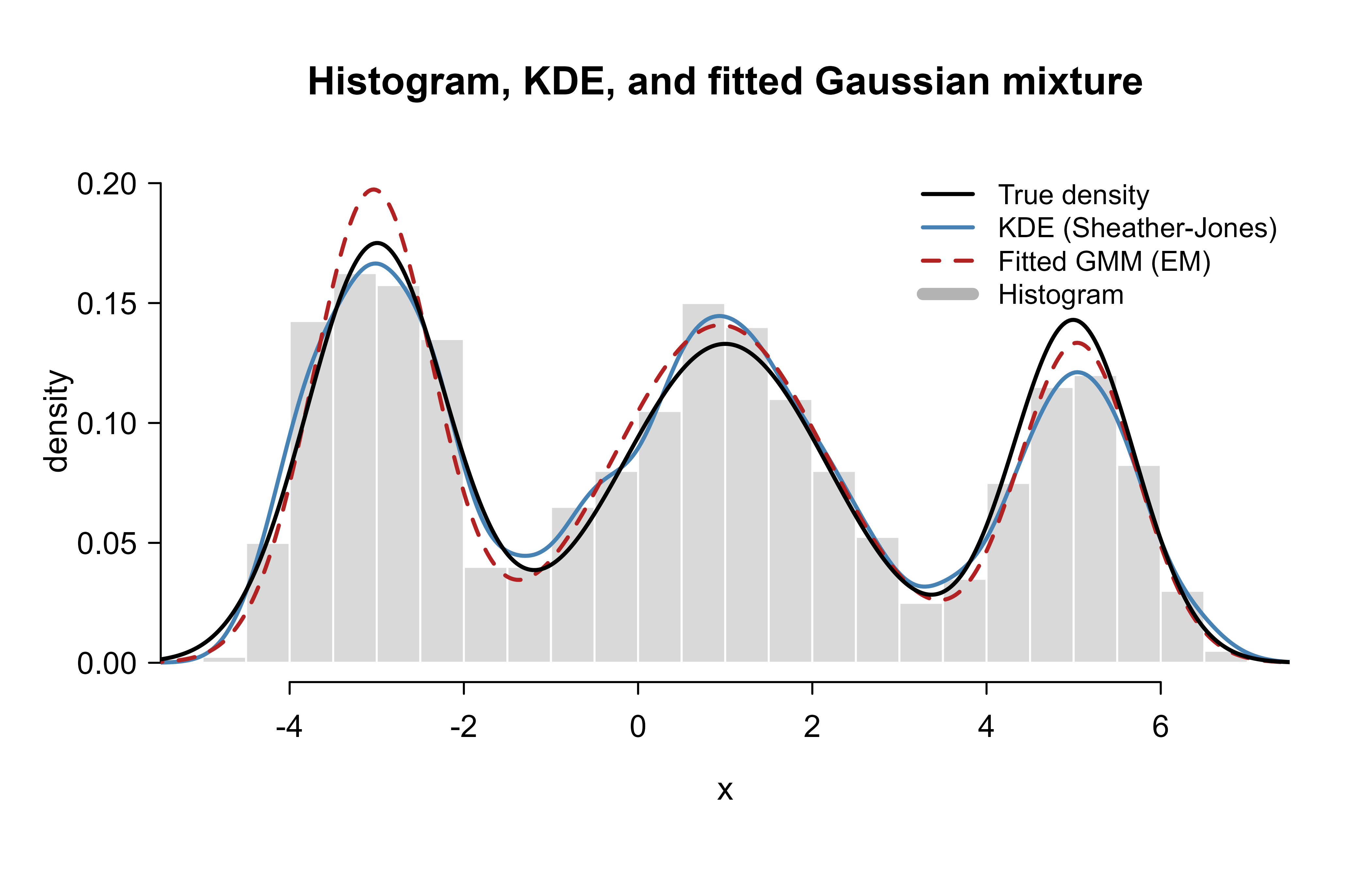
The smooth methods clearly beat the histogram: both the KDE and the mixture recover the three peaks, while the histogram’s bars depend on where the bin edges happen to fall.
32.6.1 The bandwidth effect
The previous figure used one good bandwidth. To see why bandwidth is the decisive choice in KDE, Figure 32.2 shows the same sample estimated with three bandwidths: too small (undersmoothed and spiky), automatic via Sheather-Jones (about right), and too large (oversmoothed into a single blob).
Show code
h_auto <- bw.SJ(x)
kde_small <- density(x, bw = h_auto / 5)
kde_auto <- density(x, bw = h_auto)
kde_large <- density(x, bw = h_auto * 5)

plot(grid, true_p,
    type = "l", lwd = 2, col = "black",
    main = "Effect of KDE bandwidth on the same sample",
    xlab = "x", ylab = "density", ylim = c(0, max(true_p) * 1.25)
)
lines(kde_small, col = "darkorange", lwd = 1.5)
lines(kde_auto, col = "steelblue", lwd = 2)
lines(kde_large, col = "purple", lwd = 2)
legend("topright",
    legend = c(
        "True density",
        sprintf("Too small (h = %.2f)", h_auto / 5),
        sprintf("Sheather-Jones (h = %.2f)", h_auto),
        sprintf("Too large (h = %.2f)", h_auto * 5)
    ),
    col = c("black", "darkorange", "steelblue", "purple"),
    lwd = 2, bty = "n", cex = 0.85
)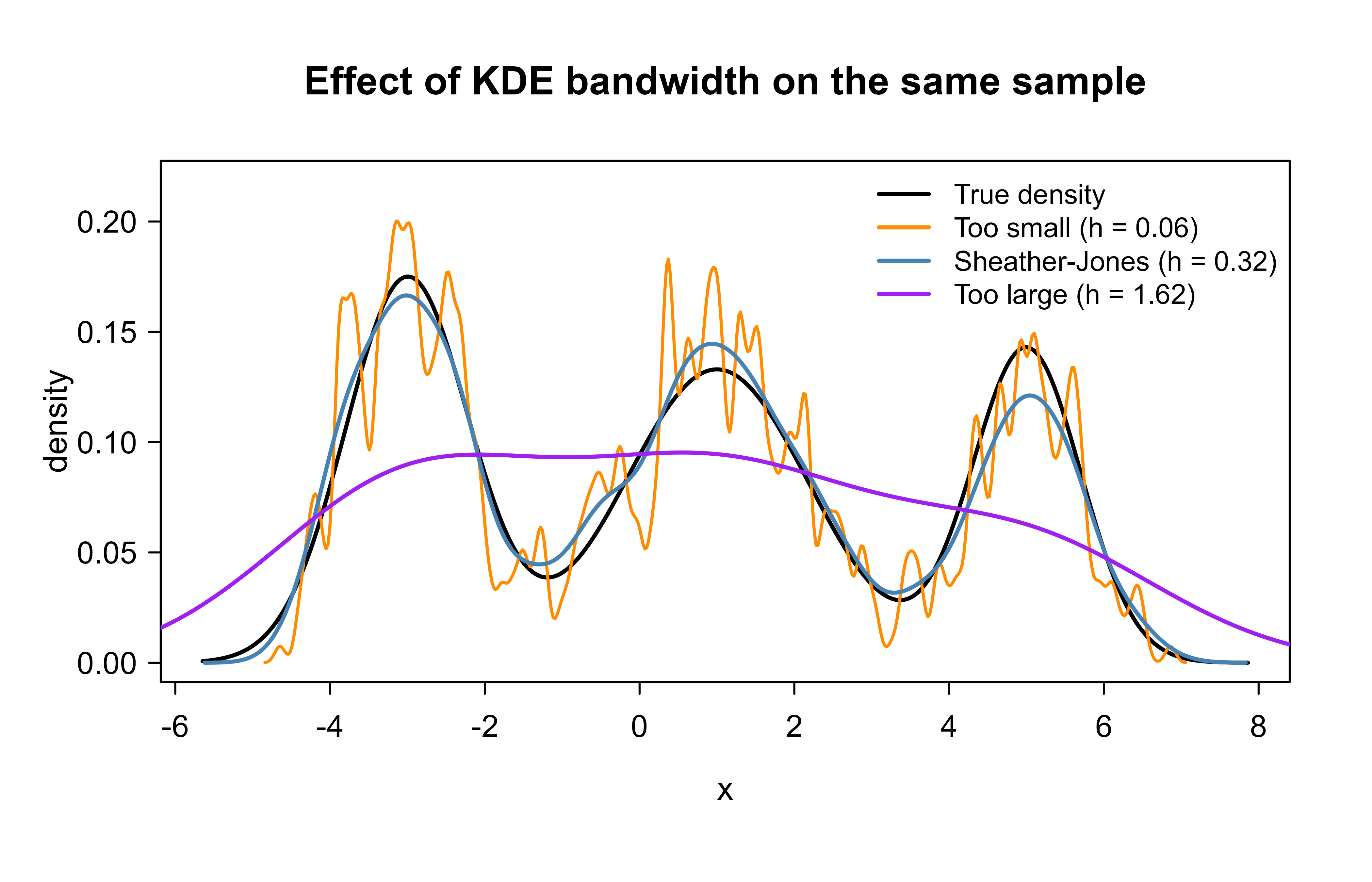
The lesson is visible at a glance: the orange curve chases individual data points and reports modes that are not real, while the purple curve has smoothed the genuine three-peak structure into a single uninformative bump. Only the middle bandwidth tells the truth.
32.7 A scikit-style flow sketch (not run)
For completeness, the conceptual training loop for a normalizing flow is shown below. It needs a deep-learning backend, so it is not executed here; it illustrates the change-of-variables loss in idiomatic pseudocode.
Show code
# Conceptual only: requires the torch backend (not run in this book build).
# A normalizing flow maximizes the exact log-likelihood via change of variables.

library(torch)

# A coupling layer transforms half the coordinates as a function of the other
# half, giving a triangular Jacobian whose log-determinant is cheap.
coupling_forward <- function(x, net) {
    d <- ncol(x) %/% 2
    x1 <- x[, 1:d]
    x2 <- x[, (d + 1):ncol(x)]
    st <- net(x1) # network outputs scale (s) and shift (t)
    s <- st$scale
    t <- st$shift
    y2 <- x2 * torch_exp(s) + t # affine transform of the second half
    list(y = torch_cat(list(x1, y2), dim = 2), log_det = s$sum(dim = 2))
}

# Training: push data to the base space, accumulate log-determinants,
# and maximize log p(x) = log N(z; 0, I) + sum(log|det J|).
flow_nll <- function(x, layers) {
    z <- x
    log_det_total <- torch_zeros(nrow(x))
    for (layer in layers) {
        out <- coupling_forward(z, layer)
        z <- out$y
        log_det_total <- log_det_total + out$log_det
    }
    log_pz <- distr_normal(0, 1)$log_prob(z)$sum(dim = 2)
    -(log_pz + log_det_total)$mean() # negative log-likelihood to minimize
}
32.8 Practical guidance and pitfalls
A few hard-won rules separate a useful density estimate from a misleading one.
Match the method to the dimension. In one or two dimensions, plot a KDE and trust your eyes; in moderate dimensions, fit a Gaussian mixture and select \(K\) by BIC; in high dimensions, abandon nonparametric methods and use a parametric or neural model, because the curse of dimensionality makes KDE meaningless. A KDE in ten dimensions is not a slightly-worse estimate, it is essentially no estimate at all.
Respect the support of the variable. KDE and Gaussians put mass on the whole real line, so a kernel estimate of a strictly positive quantity (a price, a duration) will leak probability below zero and create a spurious bump near the boundary. The standard fixes are to transform first (estimate the density of \(\log x\) and back-transform with the Jacobian) or to use a boundary-corrected kernel.
Choose the bandwidth deliberately. The default rule (Silverman) oversmooths multimodal data because it assumes one Gaussian; prefer the Sheather-Jones plug-in (bw.SJ) or cross-validation (bw.ucv) when you suspect multiple modes. Always look at the estimate under two or three bandwidths before believing any feature.
Beware the singularities of the mixture likelihood. A Gaussian component that collapses onto one point sends the likelihood to infinity; regularize the covariances, use several random restarts, and prefer the lower-BIC fit rather than the highest-likelihood one.
Finally, remember what the density is for. If the downstream task is anomaly detection, you do not need the density to be accurate everywhere, only to be reliably small in the tails where anomalies live; a crude global fit with well-behaved tails can beat a wiggly fit that nails the bulk but produces erratic tail values.
Table 32.2 summarizes the trade-offs across the four approaches.
Show code
methods_tab <- data.frame(
    Method = c("Histogram", "Kernel density (KDE)", "Gaussian mixture (EM)", "Normalizing flow"),
    Type = c("Nonparametric", "Nonparametric", "Parametric", "Neural / parametric"),
    `Smoothing knob` = c("Bin width h", "Bandwidth h", "Components K", "Network capacity"),
    `Good dimension` = c("1", "1 to 2", "Up to dozens", "Hundreds+"),
    `Exact likelihood` = c("Yes", "Yes", "Yes", "Yes"),
    `Can sample` = c("Crudely", "Yes", "Yes", "Yes"),
    check.names = FALSE
)
knitr::kable(
    methods_tab,
    caption = "Comparison of density estimation methods. Nonparametric methods make few assumptions but fail in high dimensions; the Gaussian mixture is compact and interpretable in moderate dimensions; normalizing flows scale to high dimensions at the cost of training a neural network."
)| Method | Type | Smoothing knob | Good dimension | Exact likelihood | Can sample |
|---|---|---|---|---|---|
| Histogram | Nonparametric | Bin width h | 1 | Yes | Crudely |
| Kernel density (KDE) | Nonparametric | Bandwidth h | 1 to 2 | Yes | Yes |
| Gaussian mixture (EM) | Parametric | Components K | Up to dozens | Yes | Yes |
| Normalizing flow | Neural / parametric | Network capacity | Hundreds+ | Yes | Yes |
32.9 Further reading
Silverman (1986), Density Estimation for Statistics and Data Analysis, is the classic and still readable account of histograms and kernel methods, including the bias-variance analysis and the rule-of-thumb bandwidth. Scott (2015), Multivariate Density Estimation, extends this to higher dimensions and is the source of Scott’s rule. Wand and Jones (1995), Kernel Smoothing, give the careful treatment of bandwidth selection, including the Sheather-Jones plug-in.
For mixtures and EM, McLachlan and Peel (2000), Finite Mixture Models, is the standard reference, and the original EM paper is Dempster, Laird, and Rubin (1977). Bishop (2006), Pattern Recognition and Machine Learning, gives a particularly clear derivation of EM for Gaussian mixtures via the evidence lower bound, connecting it to the variational methods in the generative models chapter (Chapter 42).
For normalizing flows, Rezende and Mohamed (2015) introduced the framework for variational inference, Dinh, Sohl-Dickstein, and Bengio (2017) presented RealNVP, and the survey by Papamakarios, Nalisnick, Rezende, Mohamed, and Lakshminarayanan (2021), Normalizing Flows for Probabilistic Modeling and Inference, is the comprehensive modern overview.
This is why the histogram and KDE in this chapter are presented in one dimension, the parametric Gaussian mixture is the workhorse in moderate dimensions, and normalizing flows are the tool of choice when \(d\) is in the hundreds or thousands, as for images.↩︎