Most predictive models return a point estimate \(\hat{y}\) and stop there. In production, the more useful question is often not “what is the prediction?” but “how much should I trust this prediction?” A credit model that is confident on applicants similar to its training data and uncertain on applicants from a new region behaves very differently from one that reports the same confidence everywhere. Uncertainty quantification (UQ) is the set of tools that attaches a calibrated sense of doubt to model outputs.
This chapter covers the practical core of Bayesian deep learning and UQ for data scientists and ML engineers who work in R: the distinction between aleatoric and epistemic uncertainty, and the four methods that show up most often in practice, namely Monte Carlo (MC) dropout, deep ensembles, the Laplace approximation, and variational inference. The runnable demonstrations use base R and installed packages so the ideas are concrete. The deep learning code that needs Keras or Torch is shown as correct, idiomatic code but is not executed here.
By the end you will be able to name and motivate the two kinds of uncertainty, read the one formula that ties them together (the law of total variance), pick a UQ method that fits your constraints, and run a small ensemble in plain R that produces calibrated predictive intervals. The chapter builds on the Bayesian regression and Gaussian process material from earlier and connects forward to any model where a prediction alone is not enough.
Intuition
A point prediction is a confident assertion with no escape hatch. UQ turns “the answer is 7” into “the answer is probably between 5 and 9, and I am especially unsure out here because I have never seen inputs like this.” The second statement is far more useful for any decision that has a cost attached to being wrong.
46.1 Where this fits in a modern ML workflow
A standard supervised pipeline produces a function \(f_\theta(x)\) trained by minimizing a loss. UQ sits at two points in that pipeline.
At training time, it changes how you fit the model (Bayesian priors, dropout kept on, an ensemble of fits) so that the model can express uncertainty at all.
At serving time, it changes what you return: a predictive distribution \(p(y \mid x)\) or an interval, instead of a single number.
Downstream consumers use this in concrete ways. Active learning (Chapter 50) queries the points where epistemic uncertainty is highest. Out-of-distribution detection, closely related to anomaly detection (Chapter 87), flags inputs where the model is uncertain because they look unlike anything in training. Risk-sensitive decisions (medical triage, autonomous control, pricing) use the predictive variance directly in an expected-cost calculation. Selective prediction abstains when uncertainty exceeds a threshold and routes the case to a human.1
When to use this
Reach for UQ whenever a wrong prediction has a cost that depends on how wrong it is, whenever you need to decide where to collect more data, or whenever the model will face inputs that may not resemble its training set. If every prediction is cheap and the data is stationary, a point estimate may be all you need.
46.2 Two kinds of uncertainty
The central conceptual split is between aleatoric and epistemic uncertainty. They behave differently and call for different remedies, so keeping them separate is worth the effort.
Aleatoric uncertainty is the noise inherent in the data-generating process. If you measure the same \(x\) many times and get different \(y\) values, that spread is aleatoric. It does not shrink as you collect more data, because it is a property of the world (sensor noise, intrinsic randomness, unmeasured covariates). In a regression model with response
the term \(\sigma^2(x)\) is the aleatoric variance. When it depends on \(x\) it is called heteroscedastic2; a model can learn \(\sigma^2(x)\) as a second output head.
Epistemic uncertainty is uncertainty about the model itself: which parameters \(\theta\), or even which function \(f\), generated the data. It is large where you have little data and shrinks toward zero as data accumulates. In the Bayesian view, epistemic uncertainty is encoded in the posterior over parameters \(p(\theta \mid \mathcal{D})\), where \(\mathcal{D} = \{(x_i, y_i)\}_{i=1}^n\) is the training set.
Key idea
Aleatoric is noise in the world and will not go away with more data; epistemic is doubt in the model and shrinks as data accumulates. A useful one-word test: if collecting more samples at this input would tighten the prediction, the uncertainty is epistemic; if it would not, it is aleatoric.
The Bayesian predictive distribution makes the decomposition explicit. The posterior predictive for a new input \(x_*\) is
The inner term \(p(y_* \mid x_*, \theta)\) carries aleatoric noise; the spread of \(\theta\) under the posterior carries epistemic uncertainty. Using the law of total variance, the total predictive variance splits as
The first term averages the noise variance over the posterior; the second measures how much the mean prediction moves as \(\theta\) varies. This formula is the practical workhorse of the chapter: every method below is, in effect, a recipe for sampling or approximating \(p(\theta \mid \mathcal{D})\) so that you can estimate these two terms.
46.2.1 Deriving the variance decomposition
The split above is the law of total variance specialized to the posterior predictive, and it is worth deriving once so the two terms are unambiguous. Write \(m(\theta) = E(y_* \mid x_*, \theta)\) for the conditional mean and \(v(\theta) = \operatorname{Var}(y_* \mid x_*, \theta)\) for the conditional (aleatoric) variance, with both conditioned implicitly on \(x_*\), and let expectations \(E_\theta\) and variances \(\operatorname{Var}_\theta\) be taken over the posterior \(p(\theta \mid \mathcal{D})\). Start from the definition of variance applied to the marginal predictive,
Square and take the joint expectation over \((\theta, y_*)\). The cross term vanishes because, conditional on \(\theta\), \(E[(y_* - m(\theta)) \mid \theta] = 0\) while \((m(\theta) - \bar m)\) is \(\theta\)-measurable:
Two consequences are worth stating. The epistemic term Equation 46.1 is nonnegative and shrinks to zero exactly when the posterior concentrates on a single \(\theta\), which under standard regularity (a well-specified model, an identifiable parameter, and a prior with mass near the truth) happens as \(n \to \infty\) by posterior consistency. The aleatoric term does not depend on \(n\) and persists at the irreducible noise floor. This is the precise sense in which “more data removes epistemic but not aleatoric” uncertainty.
Note
If you remember one equation from this chapter, make it the law-of-total-variance split above. Once you can sample plausible parameter settings \(\theta\) from (an approximation of) the posterior, the rest is bookkeeping: average each member’s noise for the aleatoric piece, and measure the scatter of the members’ means for the epistemic piece.
46.3 The four practical methods
The exact integral over \(p(\theta \mid \mathcal{D})\) is intractable for any non-trivial network, so all methods are approximations. They trade off accuracy, compute, and how much they disturb your existing training code. The four below are ordered roughly from least to most intrusive: deep ensembles change only how many times you train, MC dropout changes nothing at all, Laplace bolts on after training, and variational inference rewrites the layers. Read each in three parts: the one-sentence idea, the formula that makes it precise, and the practical catch.
46.3.1 Deep ensembles
Train \(M\) networks independently from different random initializations (and, often, different data shuffles or bootstrap resamples). Each fit \(\theta^{(m)}\) lands in a different mode of the loss surface. Treat the collection as samples that approximate the posterior. The predictive mean and epistemic variance are
If each network also outputs a variance \(\sigma^2_{\theta^{(m)}}(x_*)\), add its mean to get total variance. Ensembles are simple, embarrassingly parallel, and tend to give the best-calibrated uncertainty in benchmarks. The cost is \(M\) times the training and storage.
46.3.1.1 Why a variance head needs the Gaussian NLL, and what it estimates
The heteroscedastic variance head in the Keras template below is trained by minimizing the Gaussian negative log-likelihood, and it is worth seeing why that loss recovers the noise variance rather than collapsing. With outputs \(\mu_\theta(x)\) and \(\sigma^2_\theta(x)\) the per-point negative log-likelihood is, up to a constant,
Hold the mean fixed and minimize over the variance at a single input. Writing \(s = \sigma^2_\theta(x)\) and \(r^2 = (y - \mu_\theta(x))^2\), set \(\partial \ell / \partial s = \tfrac{1}{2s} - \tfrac{r^2}{2 s^2} = 0\), which gives \(\hat s = r^2\). Aggregated over points sharing similar \(x\), the optimal head therefore reports the local mean squared residual, which is exactly the conditional noise variance \(\sigma^2(x)\) that defines aleatoric uncertainty. The \(\tfrac{1}{2}\log s\) term is what prevents the degenerate solution \(s \to \infty\) (which would zero out the data term): it penalizes inflating the variance, so the two terms balance at the true residual scale. In practice one parameterizes the head by \(\log \sigma^2_\theta(x)\) (as in the template) so the output is unconstrained and \(\exp(-\log s)\) is numerically stable, which is the precise role of the tf$exp(-logvar) factor in the code.
Tip
Because the \(M\) fits are independent, you can train them on separate machines or GPUs at the same time. That makes ensembles the easiest UQ method to scale when you have hardware but not much patience for new code.
46.3.2 MC dropout
Dropout randomly zeroes activations with probability \(p\) during training as a regularizer. The MC dropout idea is to keep dropout on at prediction time and run \(T\) stochastic forward passes. Each pass uses a different random mask, equivalent to sampling a different sub-network, so the spread across passes approximates epistemic uncertainty:
where \(z_t\) is the random dropout mask on pass \(t\). This is almost free to add to an existing dropout network: no retraining, just turning off the usual “eval mode” deactivation of dropout. The catch is that the implied posterior is tied to the dropout rate and is often poorly calibrated unless the rate is tuned.
Monte Carlo error of the sample estimators
Both MC dropout and the ensemble combine \(T\) (or \(M\)) stochastic predictions, so their estimates carry Monte Carlo error on top of the modeling error. The sample mean \(\widehat{E}(y_*\mid x_*)\) has standard error \(\operatorname{sd}_{\text{epi}}(x_*)/\sqrt{T}\), so it tightens as \(T^{-1/2}\); the sample variance estimator of the epistemic term itself converges at the same \(T^{-1/2}\) rate but with larger constant (its relative error is roughly \(\sqrt{2/(T-1)}\) for Gaussian draws). The practical reading is that \(T\) in the low hundreds pins down the predictive mean cheaply, but stable variance and tail quantiles want more passes. This MC error is distinct from and additional to the bias of the underlying posterior approximation.
46.3.2.1 MC dropout as variational inference
MC dropout is not an ad hoc trick: it is exact variational inference under a specific approximating family. The argument (Gal and Ghahramani, 2016) treats each weight matrix \(W_\ell\) of layer \(\ell\) as random and uses the variational distribution
where \(M_\ell\) is the learned weight matrix and \(z_\ell\) are the dropout masks. This \(q_\phi\), a mixture of two Gaussians per weight with one component pinned near zero, is the family whose ELBO is being maximized. The reconstruction term of the ELBO is
which is precisely averaging the data log-likelihood over \(T\) dropout masks. With an L2 weight penalty of strength \(\lambda\) standing in for the KL-to-prior term, minimizing the usual dropout training objective is therefore (approximately) maximizing the ELBO. The same masks at test time then turn the trained network into a sampler from \(q_\phi\), and Equation 46.1 supplies the variance decomposition. This derivation also exposes the method’s structural limitation: because the Bernoulli rate \(p\) is fixed, the predictive variance has a floor that does not vanish as \(n \to \infty\), so MC dropout cannot in general be posterior-consistent for epistemic uncertainty without annealing \(p\) with the data.
Warning
MC dropout is cheap precisely because it reuses one set of weights, so its uncertainty does not necessarily shrink to zero even with unlimited data. Treat it as a useful rough signal, not a calibrated posterior, unless you have validated the dropout rate against held-out coverage.
46.3.3 Laplace approximation
Fit the network normally to the maximum-a-posteriori (MAP) estimate \(\hat\theta\), then approximate the posterior near that mode with a Gaussian. A second-order Taylor expansion of the log-posterior \(\log p(\theta \mid \mathcal{D})\) around \(\hat\theta\) gives
where \(H\) is the Hessian of the negative log-posterior at the mode (often approximated by the Fisher information or a Kronecker-factored block-diagonal version, since the full Hessian is too large).3 It is cheap because it reuses the trained weights and only adds a curvature estimate, and modern “last-layer” Laplace applies the Gaussian only to the final layer to keep \(H\) small.
46.3.3.1 Deriving the Laplace Gaussian
Let \(g(\theta) = \log p(\theta \mid \mathcal{D}) = \log p(\mathcal{D}\mid\theta) + \log p(\theta) - \log p(\mathcal{D})\). The MAP estimate \(\hat\theta\) is a stationary point, so \(\nabla g(\hat\theta) = 0\). A second-order Taylor expansion of \(g\) about \(\hat\theta\) has no first-order term,
\[
g(\theta) \approx g(\hat\theta) - \tfrac{1}{2}(\theta - \hat\theta)^\top H (\theta - \hat\theta),
\qquad H = -\nabla^2_\theta g(\hat\theta) ,
\]
so exponentiating gives \(p(\theta\mid\mathcal{D}) \propto \exp\!\big(-\tfrac12 (\theta-\hat\theta)^\top H (\theta-\hat\theta)\big)\), the kernel of a \(N(\hat\theta, H^{-1})\) density (and \(H \succ 0\) at a maximum guarantees a valid covariance). This is the multivariate Laplace method: a Gaussian fit by matching the mode and the curvature there. As a byproduct, integrating the unnormalized posterior under the same quadratic gives the Laplace estimate of the log marginal likelihood,
with \(d = \dim(\theta)\); the \(-\tfrac12\log\det H\) term is an Occam factor that rewards flat (low-curvature) modes and is what makes Laplace usable for hyperparameter selection.
46.3.3.2 From parameter posterior to predictive: the linearized variance
For a regression output \(f_\theta(x_*)\) the Laplace posterior on \(\theta\) must be pushed through \(f\) to get a predictive variance. A first-order (delta-method) expansion around the mode, \(f_\theta(x_*) \approx f_{\hat\theta}(x_*) + J_*^\top (\theta - \hat\theta)\) with Jacobian \(J_* = \nabla_\theta f_\theta(x_*)\big|_{\hat\theta}\), makes the output marginally Gaussian:
This “linearized Laplace” is the form implemented in practice and is what the torch sketch computes. For the last-layer variant the network body is frozen, so \(f_\theta(x_*) = \phi(x_*)^\top w\) is linear in the last-layer weights \(w\), the Jacobian is exactly the frozen features \(J_* = \phi(x_*)\), and Equation 46.3 becomes \(\phi(x_*)^\top H^{-1}\phi(x_*) + \sigma^2\), identical in form to the Bayesian linear regression predictive variance derived in Chapter 46 below. The generalized Gauss-Newton approximation \(H \approx \sum_i J_i J_i^\top / \sigma^2 + I/\tau^2\) replaces the true Hessian with an outer-product (Fisher) form that is always positive semidefinite, which is why it is preferred over the raw Hessian.
46.3.4 Variational inference (brief)
Variational inference (VI) replaces the intractable posterior with a tractable family \(q_\phi(\theta)\), typically a factorized Gaussian, and fits \(\phi\) by maximizing the evidence lower bound (ELBO):
The first term rewards fitting the data; the KL term keeps \(q_\phi\) close to the prior and acts as a complexity penalty. “Bayes by Backprop” makes this differentiable with the reparameterization trick so it trains with the usual stochastic gradient tooling. VI gives a genuine approximate posterior in one training run, but the factorized Gaussian usually underestimates variance and the implementation is more involved than the other three.
46.3.4.1 Why the ELBO is a lower bound
The ELBO is not an arbitrary objective; it is the log evidence minus the gap to the true posterior. Start from the log marginal likelihood and insert \(q_\phi\),
which is exactly the ELBO. The slack in the bound is the posterior approximation error: an algebraic rearrangement gives \(\log p(\mathcal{D}) - \mathcal{L}(\phi) = \operatorname{KL}\!\big(q_\phi(\theta)\,\|\,p(\theta\mid\mathcal{D})\big) \ge 0\). Maximizing the ELBO over \(\phi\) is therefore equivalent to minimizing the reverse KL from \(q_\phi\) to the true posterior. That reverse direction is precisely why mean-field VI underestimates variance: reverse KL is mode-seeking and penalizes placing mass where the posterior is small, so \(q_\phi\) shrinks to fit inside a single mode rather than covering the full posterior spread.
46.3.4.2 The reparameterization trick
The obstacle to gradient training is that \(\phi\) appears in the distribution the expectation is taken over, so \(\nabla_\phi E_{q_\phi}[\,\cdot\,]\) cannot be moved inside the expectation directly. For a factorized Gaussian \(q_\phi(\theta) = N(\mu, \operatorname{diag}(\sigma^2))\) with \(\phi = (\mu, \rho)\) and \(\sigma = \log(1+e^{\rho})\), write the sample as a deterministic transform of parameter-free noise,
A single sample (\(S = 1\)) per minibatch usually suffices. This Monte Carlo gradient is unbiased and typically far lower variance than the score-function (REINFORCE) estimator, which is what makes Bayes by Backprop trainable with ordinary SGD. The KL term against a Gaussian prior \(N(0,\tau^2 I)\) has the closed form \(\operatorname{KL} = \tfrac12\sum_j\big(\sigma_j^2/\tau^2 + \mu_j^2/\tau^2 - 1 - \log(\sigma_j^2/\tau^2)\big)\), so only the data term needs sampling.
46.3.5 Comparison
Table 46.1 lays the four methods side by side so the trade-offs are easy to scan.
Table 46.1: Comparison of the four practical uncertainty quantification methods across posterior approximation, compute cost, what they capture, calibration, and how much they disturb existing training code.
Method
Posterior approximation
Extra training cost
Extra inference cost
Captures
Calibration in practice
Code intrusiveness
Deep ensembles
\(M\) modes (samples)
\(\times M\)
\(\times M\) forward passes
Epistemic (+ aleatoric if variance head)
Usually best
Low (train loop \(M\) times)
MC dropout
Implicit, dropout-induced
None (reuse model)
\(\times T\) forward passes
Epistemic, rate-dependent
Fair, needs tuning
Very low
Laplace
Gaussian at the mode
Small (curvature)
Small (last-layer) to moderate
Epistemic (local)
Good if curvature is reliable
Low (post-hoc)
Variational inference
Tractable family \(q_\phi\)
Comparable to one fit
\(\times T\) samples
Epistemic
Often underestimates
High (rewrite layers)
Reading the table by column tells you what you are buying. The “code intrusiveness” column is the one that most often decides the choice in practice: a method you can add in an afternoon beats a theoretically nicer one that takes a week, especially for a first pass. A common default follows from this:
Start with a small deep ensemble (\(M = 5\)); it is the strongest baseline and the easiest to reason about.
Reach for MC dropout when retraining is impossible and the model already has dropout layers.
Use last-layer Laplace when you need cheap post-hoc intervals on an already-trained model.
Use VI when memory rules out an ensemble and you can afford the engineering.
With the methods surveyed, the next two sections make the ideas concrete in plain R, first by resampling (a bootstrap ensemble) and then in closed form (Bayesian linear regression).
46.4 Runnable demo: bootstrap deep ensemble for predictive intervals
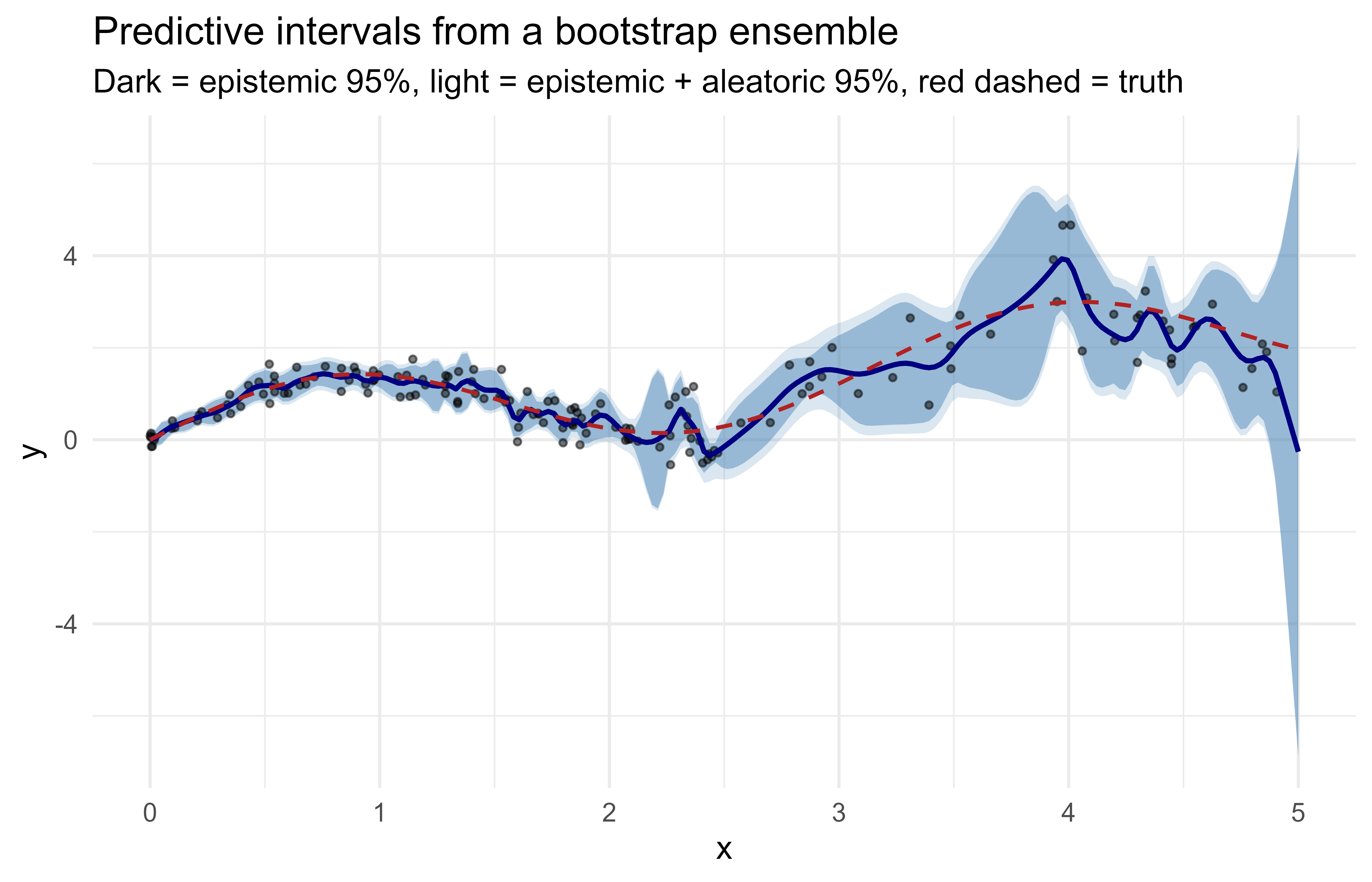
The cleanest way to see the aleatoric/epistemic split without a GPU is a bootstrap ensemble of flexible regressors. A bootstrap resample draws \(n\) rows from the training set with replacement, so each member sees a slightly different dataset and lands on a slightly different fitted function. That collection of functions plays the role of samples from the posterior: a different \(\theta^{(m)}\) per member. The spread of member means is then epistemic, and the residual noise around the truth is aleatoric.
To make both kinds of uncertainty visible at once, we rig the data deliberately. The noise grows with \(x\) (heteroscedastic), so the aleatoric part should widen to the right regardless of how much data we have. And we make the data sparse beyond \(x = 2.5\), so the epistemic part should widen on the right because the members disagree where they have few points to anchor them. A good UQ method should pick up both effects.
Intuition
Bootstrapping is a poor person’s posterior. We cannot enumerate every plausible model, so we perturb the data and refit many times; the wobble in the resulting predictions stands in for our uncertainty about which model is right.
Show code
set.seed(42)# Heteroscedastic truth: noise grows with x. Data is dense on the left,# sparse on the right, so epistemic uncertainty should grow to the right.f_true<-function(x)sin(2*x)+0.5*xsd_noise<-function(x)0.10+0.18*x# aleatoric sd grows with xn<-160x<-c(runif(120, 0, 2.5), runif(40, 2.5, 5))# sparse beyond x = 2.5y<-f_true(x)+rnorm(n, 0, sd_noise(x))dat<-data.frame(x =x, y =y)grid<-data.frame(x =seq(0, 5, length.out =200))# Bootstrap ensemble of smoothing splines. Each member sees a resample,# giving a different fitted function (a draw of theta).M<-200fits<-matrix(NA_real_, nrow =nrow(grid), ncol =M)for(minseq_len(M)){idx<-sample.int(n, n, replace =TRUE)sm<-smooth.spline(dat$x[idx], dat$y[idx], cv =FALSE)fits[, m]<-predict(sm, grid$x)$y}# Epistemic: spread of the member mean functions.mean_pred<-rowMeans(fits)epi_var<-apply(fits, 1, var)# Aleatoric: estimate residual variance, then smooth log of squared# residuals against x so it can vary (heteroscedastic estimate).res2<-(dat$y-predict(smooth.spline(dat$x, dat$y, cv =FALSE), dat$x)$y)^2ale_model<-smooth.spline(dat$x, log(res2+1e-6), cv =FALSE)ale_var<-pmax(exp(predict(ale_model, grid$x)$y), 1e-6)# Total predictive sd from the law of total variance.total_sd<-sqrt(epi_var+ale_var)head(data.frame(x =grid$x, mean =mean_pred, epi_sd =sqrt(epi_var), ale_sd =sqrt(ale_var)))#> x mean epi_sd ale_sd#> 1 0.00000000 0.009162608 0.09693522 0.05078014#> 2 0.02512563 0.042250679 0.08808231 0.05281048#> 3 0.05025126 0.144213643 0.11858262 0.05492543#> 4 0.07537688 0.230213761 0.09235935 0.05712907#> 5 0.10050251 0.293256817 0.06674870 0.05942512#> 6 0.12562814 0.340124616 0.08430585 0.06181662
Figure 46.1 shows the decomposition. The dark band is epistemic only; the lighter band adds aleatoric noise to give a 95% predictive interval. Notice the epistemic band widens where data is sparse (right side), while the aleatoric band widens with \(x\) regardless of data density.
Show code
library(ggplot2)band<-data.frame( x =grid$x, mean =mean_pred, epi_lo =mean_pred-1.96*sqrt(epi_var), epi_hi =mean_pred+1.96*sqrt(epi_var), tot_lo =mean_pred-1.96*total_sd, tot_hi =mean_pred+1.96*total_sd, truth =f_true(grid$x))ggplot()+geom_ribbon(data =band, aes(x, ymin =tot_lo, ymax =tot_hi), fill ="steelblue", alpha =0.20)+geom_ribbon(data =band, aes(x, ymin =epi_lo, ymax =epi_hi), fill ="steelblue", alpha =0.45)+geom_point(data =dat, aes(x, y), size =0.9, alpha =0.5)+geom_line(data =band, aes(x, mean), color ="navy", linewidth =0.9)+geom_line(data =band, aes(x, truth), color ="firebrick", linetype ="dashed", linewidth =0.7)+labs(x ="x", y ="y", title ="Predictive intervals from a bootstrap ensemble", subtitle ="Dark = epistemic 95%, light = epistemic + aleatoric 95%, red dashed = truth")+theme_minimal(base_size =12)
Figure 46.1: Bootstrap deep ensemble. Epistemic uncertainty (dark band) grows where training data is sparse; aleatoric noise (light band) grows with x by construction.
The printed table confirms the intended behavior at a glance: the epistemic standard deviation (epi_sd) and aleatoric standard deviation (ale_sd) are reported separately for each grid point, so you can see the two pieces before they are combined into the total band.
A figure is persuasive but not proof. The honest test of any UQ method is calibration: a 95% predictive interval should contain close to 95% of fresh, held-out points. We check that directly on new data drawn from the same process.
Show code
# Coverage check on fresh test data drawn from the same process.set.seed(7)x_te<-runif(2000, 0, 5)y_te<-f_true(x_te)+rnorm(2000, 0, sd_noise(x_te))# Interpolate the fitted mean and total sd onto the test inputs.mu_te<-approx(grid$x, mean_pred, xout =x_te, rule =2)$ysd_te<-approx(grid$x, total_sd, xout =x_te, rule =2)$ylo<-mu_te-1.96*sd_tehi<-mu_te+1.96*sd_tecoverage<-mean(y_te>=lo&y_te<=hi)round(coverage, 3)# target is about 0.95#> [1] 0.834
The observed coverage lands somewhat below the nominal 95%, which is itself instructive. The aleatoric variance here is estimated by smoothing squared residuals, a deliberately rough plug-in that tends to undershoot the true noise, so the bands come out a little too narrow. This is exactly why the calibration check matters: a plausible-looking figure can still be overconfident, and only held-out coverage reveals it.
Warning
Never judge an uncertainty method by how tight its bands look. Tight and wrong is worse than wide and honest. Always pair a figure with a numeric coverage or scoring-rule check on data the model did not see.
46.5 Runnable demo: Bayesian linear regression posterior predictive
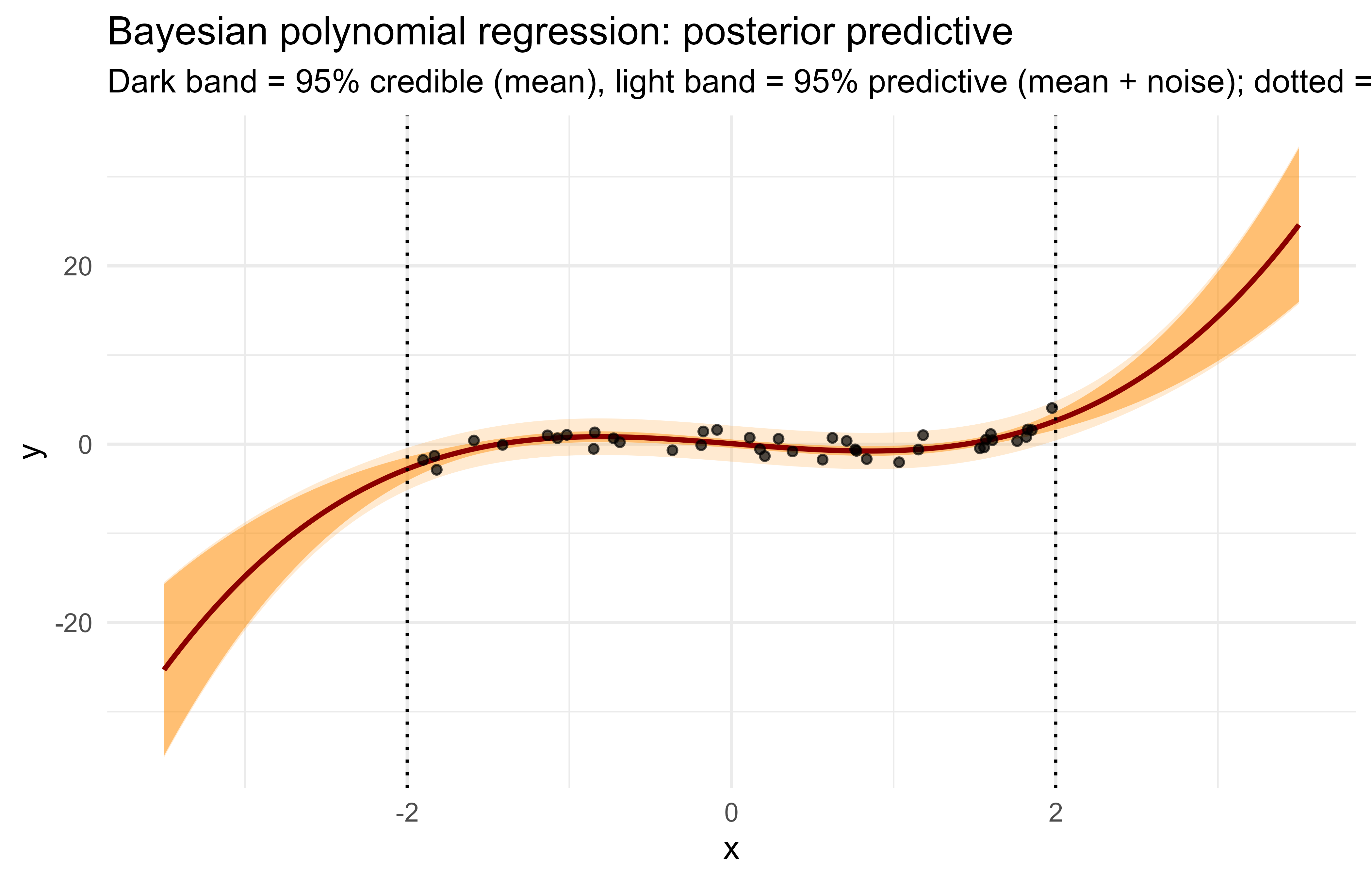
For a model where the posterior is available in closed form, we can show credible bands exactly rather than by resampling. Bayesian linear regression with a conjugate Gaussian prior is the canonical example, and it makes the aleatoric/epistemic split fully analytic.
Take the model \(y = X\beta + \epsilon\) with \(\epsilon \sim N(0, \sigma^2 I)\), a known \(\sigma^2\) for simplicity, and a Gaussian prior \(\beta \sim N(0, \tau^2 I)\). The posterior over coefficients is Gaussian,
To derive Equation 46.4, multiply the Gaussian likelihood by the Gaussian prior and read off the exponent as a quadratic in \(\beta\) (the conjugate “complete the square” argument). Dropping terms not involving \(\beta\), the log posterior is
A Gaussian \(N(\mu_n,\Sigma_n)\) has log density with quadratic coefficient \(-\tfrac12\Sigma_n^{-1}\) and linear coefficient \(\Sigma_n^{-1}\mu_n\). Matching the two displays gives \(\Sigma_n = (\tfrac{1}{\sigma^2}X^\top X + \tfrac{1}{\tau^2}I)^{-1}\) and \(\mu_n = \tfrac{1}{\sigma^2}\Sigma_n X^\top y\) at once. The posterior mean is the ridge estimate with penalty \(\sigma^2/\tau^2\), which exhibits the prior as the regularizer: a tight prior (small \(\tau^2\)) shrinks \(\beta\) harder. As \(n\) grows, \(X^\top X = O(n)\) dominates the \(I/\tau^2\) term, so \(\Sigma_n = O(1/n)\) and the prior washes out, the Bernstein-von Mises behavior for this model.
For a new input row \(x_*\), the posterior predictive is Gaussian with
The two variance terms are exactly the decomposition from the law of total variance, with the epistemic term shrinking as \(X^\top X\) grows with more data. The aleatoric term \(\sigma^2\) is constant here because we assumed homoscedastic noise. We use a polynomial basis so the mean function can curve.
The predictive variance follows directly from Equation 46.4 by writing \(y_* = x_*^\top\beta + \epsilon_*\) with \(\epsilon_* \sim N(0,\sigma^2)\) independent of \(\beta\mid\mathcal{D}\). Then \(x_*^\top\beta \mid \mathcal{D} \sim N(x_*^\top\mu_n,\ x_*^\top\Sigma_n x_*)\) as a linear image of a Gaussian, and adding the independent noise sums the variances:
The first term is the epistemic piece \(\operatorname{Var}_\beta[E(y_*\mid x_*,\beta)]\) and the second is the aleatoric piece \(E_\beta[\operatorname{Var}(y_*\mid x_*,\beta)]\), so this is Equation 46.1 made fully analytic. The quadratic form \(x_*^\top\Sigma_n x_*\) grows when \(x_*\) points in directions poorly covered by the rows of \(X\) (small eigenvalues of \(X^\top X\)), which is why the band fans out under extrapolation in the figure.
Key idea
This closed-form model is the reference standard the deep methods are imitating. The bootstrap ensemble above approximated \(x_*^\top \Sigma_n x_*\) by resampling; here we compute it exactly. Seeing the exact answer once makes it clear what the approximations are reaching for.
Show code
set.seed(123)# Data on a limited x-range so epistemic uncertainty blows up on extrapolation.n<-40xb<-runif(n, -2, 2)yb<-0.5*xb^3-xb+rnorm(n, 0, 1.0)sigma2<-1.0# known observation noise (aleatoric)tau2<-100# weakly informative prior on coefficientsdeg<-3# Design matrices (intercept + polynomial terms).make_X<-function(x)cbind(1, poly(x, deg, raw =TRUE))X<-make_X(xb)p<-ncol(X)# Closed-form posterior over beta.Sig_n<-solve(crossprod(X)/sigma2+diag(p)/tau2)mu_n<-(Sig_n%*%t(X)%*%yb)/sigma2# Predict on a grid that extends BEYOND the training range to show extrapolation.xg<-seq(-3.5, 3.5, length.out =200)Xg<-make_X(xg)mean_g<-as.numeric(Xg%*%mu_n)epi_var_g<-rowSums((Xg%*%Sig_n)*Xg)# x*' Sigma_n x* per rowpred_var<-epi_var_g+sigma2# add aleatoric noisebdf<-data.frame( x =xg, mean =mean_g, cred_lo =mean_g-1.96*sqrt(epi_var_g), cred_hi =mean_g+1.96*sqrt(epi_var_g), pred_lo =mean_g-1.96*sqrt(pred_var), pred_hi =mean_g+1.96*sqrt(pred_var))library(ggplot2)ggplot()+geom_ribbon(data =bdf, aes(x, ymin =pred_lo, ymax =pred_hi), fill ="darkorange", alpha =0.18)+geom_ribbon(data =bdf, aes(x, ymin =cred_lo, ymax =cred_hi), fill ="darkorange", alpha =0.45)+geom_line(data =bdf, aes(x, mean), color ="darkred", linewidth =0.9)+geom_point(data =data.frame(x =xb, y =yb), aes(x, y), size =1.3, alpha =0.7)+geom_vline(xintercept =c(-2, 2), linetype ="dotted")+labs(x ="x", y ="y", title ="Bayesian polynomial regression: posterior predictive", subtitle ="Dark band = 95% credible (mean), light band = 95% predictive (mean + noise); dotted = training range")+theme_minimal(base_size =12)
Figure 46.2: Closed-form Bayesian polynomial regression. The narrow band is the credible interval on the mean function (epistemic); the wide band is the posterior predictive interval that also includes observation noise (aleatoric).
Figure 46.2 shows the result. Outside the training range (the dotted lines), the epistemic band fans out fast: the model knows it is extrapolating. Inside the range the credible band is tight and the predictive band is dominated by the constant aleatoric floor \(\sigma^2\). This is exactly the behavior we want from a UQ method and is the gold standard the approximate deep learning methods are trying to mimic.
The closed-form epistemic variance \(x_*^\top\Sigma_n x_*\) is the population quantity the law of total variance promises. We can confirm the decomposition empirically by drawing \(\beta\) from the posterior, evaluating the mean function \(x_*^\top\beta\) for each draw, and checking that the Monte Carlo variance of those means matches the quadratic form, while the noise term adds the rest.
Show code
# Verify Var_beta[ x*' beta ] == x*' Sigma_n x* by Monte Carlo, and that# adding sigma^2 recovers the total predictive variance.set.seed(99)L<-chol(Sig_n)# Sig_n = L' LB<-50000draws_beta<-matrix(rnorm(B*p), B, p)%*%Ldraws_beta<-sweep(draws_beta, 2, as.numeric(mu_n), "+")# rows ~ N(mu_n, Sig_n)x_star<-Xg[150, ]# one extrapolation pointmean_draws<-as.numeric(draws_beta%*%x_star)mc_epi<-var(mean_draws)# Monte Carlo epistemic variancecf_epi<-as.numeric(t(x_star)%*%Sig_n%*%x_star)# closed form# Draw y* = x*'beta + noise and compare total variance.y_star_draws<-mean_draws+rnorm(B, 0, sqrt(sigma2))c(mc_epistemic =mc_epi, closed_form_epistemic =cf_epi, mc_total =var(y_star_draws), closed_form_total =cf_epi+sigma2)#> mc_epistemic closed_form_epistemic mc_total #> 0.09809957 0.09782923 1.10119300 #> closed_form_total #> 1.09782923
The Monte Carlo and closed-form columns agree to sampling error, confirming both the posterior covariance in Equation 46.4 and the variance split in Equation 46.1.
46.6 Deep learning implementations (not executed here)
The same ideas in a neural network need Keras or Torch. The code below is correct and current but is marked eval=FALSE because training is GPU-heavy and the goal here is the pattern, not the run. Read these as templates: the structure carries over directly, and the uncertainty bookkeeping at the end of each is the same law-of-total-variance split you have already seen.
MC dropout in Keras keeps dropout active at inference by calling the model in training mode:
Show code
library(keras)# A small regression network with dropout after each hidden layer.inputs<-layer_input(shape =ncol(x_train))out<-inputs|>layer_dense(64, activation ="relu")|>layer_dropout(rate =0.1)|>layer_dense(64, activation ="relu")|>layer_dropout(rate =0.1)|>layer_dense(1)model<-keras_model(inputs, out)model|>compile(optimizer ="adam", loss ="mse")model|>fit(x_train, y_train, epochs =200, batch_size =32, verbose =0)# MC dropout: run T stochastic forward passes with training = TRUE so the# dropout masks stay random at prediction time.mc_predict<-function(model, x_new, T=100){draws<-replicate(T, as.numeric(model(x_new, training =TRUE)))list(mean =rowMeans(draws), epistemic_sd =apply(draws, 1, sd))}pred<-mc_predict(model, x_test, T =200)
A deep ensemble with a variance head (so each member reports its own aleatoric noise) trained with the Gaussian negative log-likelihood:
Show code
library(keras)library(tensorflow)# Each member outputs mean and log-variance; the loss is the heteroscedastic# Gaussian NLL (Nix and Weigend, 1994; Lakshminarayanan et al., 2017).gaussian_nll<-function(y_true, y_pred){mu<-y_pred[, 1, drop =FALSE]logvar<-y_pred[, 2, drop =FALSE]0.5*tf$reduce_mean(tf$exp(-logvar)*(y_true-mu)^2+logvar)}build_member<-function(){inp<-layer_input(shape =ncol(x_train))h<-inp|>layer_dense(64, activation ="relu")|>layer_dense(64, activation ="relu")out<-layer_concatenate(list(h|>layer_dense(1), # mean headh|>layer_dense(1)# log-variance head))m<-keras_model(inp, out)m|>compile(optimizer ="adam", loss =gaussian_nll)m}M<-5members<-lapply(seq_len(M), function(i){m<-build_member()m|>fit(x_train, y_train, epochs =200, batch_size =32, verbose =0)m})# Combine members: epistemic from spread of means, aleatoric from mean of# member variances, per the law of total variance.preds<-lapply(members, function(m)as.matrix(predict(m, x_test)))mus<-sapply(preds, function(p)p[, 1])vars<-sapply(preds, function(p)exp(p[, 2]))mean_pred<-rowMeans(mus)epistemic<-apply(mus, 1, var)aleatoric<-rowMeans(vars)total_sd<-sqrt(epistemic+aleatoric)
The torch equivalent of a last-layer Laplace fit, which keeps the network’s trained body fixed and fits a Gaussian only over the final linear layer, follows the same template using nn_module and the generalized Gauss-Newton approximation to the Hessian:
Show code
library(torch)# Sketch: after standard MAP training, freeze the feature extractor and# compute the posterior precision of the last layer as# H = sum_i J_i' J_i / sigma^2 + I / tau^2# where J_i is the Jacobian of the output wrt last-layer weights at x_i.# Predictive variance at x* is then phi(x*)' H^{-1} phi(x*) + sigma^2,# with phi(x*) the frozen features. Libraries such as laplace-torch# automate this; the math matches the Laplace section above.
46.7 Practical guidance, pitfalls, and when to use each
Always validate calibration, not just sharpness. A method can produce tight, confident-looking bands that are wrong. Check empirical coverage (does the 90% interval contain 90% of held-out points?) and use proper scoring rules such as the negative log predictive density or the continuous ranked probability score. A reliability diagram for classification is the analog, covered in the probability calibration chapter (Chapter 86). The coverage check in the bootstrap demo is the minimum you should run.
46.7.1 Proper scoring rules for probabilistic predictions
Coverage checks one quantile; a proper scoring rule grades the whole predictive distribution. A scoring rule \(S(p, y)\) assigns a penalty to a predictive distribution \(p\) given the realized outcome \(y\). It is proper if the expected score is optimized (here, minimized) by reporting the true distribution: \(E_{y\sim q}\,S(q,y) \le E_{y\sim q}\,S(p,y)\) for all \(p\), and strictly proper if equality forces \(p = q\). Propriety is what makes a rule un-gameable: you cannot lower your expected penalty by being deliberately over- or under-confident, so minimizing it on held-out data simultaneously rewards calibration and sharpness.
The negative log predictive density (NLPD), \(S(p,y) = -\log p(y)\), is strictly proper. For a Gaussian predictive \(N(\mu, \sigma^2)\) it equals Equation 46.2 plus a constant, so it explicitly penalizes both a wrong mean (through \((y-\mu)^2/\sigma^2\)) and a miscalibrated spread (through the \(\tfrac12\log\sigma^2\) Occam term that punishes overconfident tiny \(\sigma\)). The continuous ranked probability score integrates the squared distance between the predictive CDF \(F\) and the step function at the outcome,
which is also strictly proper, is in the same units as \(y\) (unlike NLPD), and is finite even when the predictive density is zero at \(y\), making it more robust than NLPD to badly placed tails. For a Gaussian predictive Equation 46.5 has the closed form \(\operatorname{CRPS}(N(\mu,\sigma^2), y) = \sigma\big[\, z(2\Phi(z)-1) + 2\phi(z) - \pi^{-1/2}\big]\) with \(z = (y-\mu)/\sigma\), convenient for the variance-head and Bayesian-linear models above. Report mean NLPD or mean CRPS over the test set alongside coverage: coverage can look right while the distribution is wrong elsewhere, and a strictly proper score will catch it.
Do not confuse the two uncertainties when acting on them. High aleatoric uncertainty means “this region is inherently noisy; collecting more data will not help much.” High epistemic uncertainty means “the model has not seen enough here; more data or abstention will help.” Active learning targets epistemic; deciding whether a measurement is worth taking targets aleatoric. Reporting only total variance hides which lever to pull.
Method-specific traps.
MC dropout uncertainty is sensitive to the dropout rate and does not generally go to zero with infinite data, so treat it as a rough, cheap signal rather than a calibrated posterior. Tune the rate on a validation set.
Deep ensembles need genuine diversity. Identical initializations, identical data order, and over-regularization collapse the members onto the same solution and the epistemic band vanishes. Vary seeds and use bootstrap or different shuffles.
The Laplace approximation is only as good as its Hessian. The full Hessian is intractable for large nets, and crude diagonal approximations can be badly miscalibrated; last-layer or Kronecker-factored versions are the practical compromise. It is also a local, single-mode approximation and will miss multimodality.
Variational inference with a mean-field Gaussian systematically underestimates posterior variance because it cannot represent correlations between weights. Expect overconfidence and budget time for tuning the KL weight.
Distribution shift breaks everything. All these methods quantify uncertainty relative to the training distribution. Under genuine shift (new feature regimes, new label semantics) even well-calibrated models can be confidently wrong. Pair UQ with explicit out-of-distribution monitoring rather than assuming the predictive variance alone will catch it.
A pragmatic decision rule. If you can afford to train a handful of models, a deep ensemble of size 5 is the strong default and the hardest baseline to beat. If the model is already trained and frozen, add MC dropout (if it has dropout layers) or a last-layer Laplace fit for cheap post-hoc intervals. Reserve variational inference for cases where memory forbids an ensemble and you are prepared for the extra engineering. For small tabular problems, the closed-form Bayesian linear or Gaussian process models (Chapter 7) in the earlier chapters give exact uncertainty and should be tried before any deep method.
46.8 Summary
Three ideas carry the whole chapter. First, uncertainty comes in two flavors that demand different responses: aleatoric noise that more data cannot remove, and epistemic doubt that more data can. Second, the law of total variance splits a predictive variance cleanly into those two pieces once you can sample plausible parameter settings, which reduces every method to the same recipe of averaging member noise and measuring member disagreement. Third, the four practical methods (deep ensembles, MC dropout, Laplace, variational inference) are just different ways to produce those parameter samples, trading off compute against how much they disturb your code, and a size-5 ensemble is the default that is hardest to beat. Whichever you choose, validate it by held-out coverage rather than by how convincing the bands look, and remember that all of these methods speak only about the training distribution, so genuine distribution shift still needs separate monitoring.
46.9 Further reading
Kendall and Gal (2017), “What Uncertainties Do We Need in Bayesian Deep Learning for Computer Vision?”, on the aleatoric/epistemic decomposition.
Gal and Ghahramani (2016), “Dropout as a Bayesian Approximation”, the MC dropout paper.
Lakshminarayanan, Pritzel, and Blundell (2017), “Simple and Scalable Predictive Uncertainty Estimation using Deep Ensembles”.
Blundell, Cornebise, Kavukcuoglu, and Wierstra (2015), “Weight Uncertainty in Neural Networks” (Bayes by Backprop), for variational inference.
MacKay (1992), “A Practical Bayesian Framework for Backpropagation Networks”, the original Laplace approximation for neural networks.
Daxberger, Kristiadi, Immer, Eschenhagen, Bauer, and Hennig (2021), “Laplace Redux”, on scalable post-hoc Laplace methods.
Bishop (2006), Pattern Recognition and Machine Learning, chapters 3 and 5, for the conjugate Bayesian linear regression and Laplace foundations.
Gneiting and Raftery (2007), “Strictly Proper Scoring Rules, Prediction, and Estimation”, for evaluating probabilistic forecasts.
Selective prediction is sometimes called “reject option” classification. The model is allowed to say “I don’t know” for the hardest cases, trading coverage (the fraction of inputs it answers) for higher accuracy on the cases it does answer.↩︎
Heteroscedastic simply means “different scatter”: the noise level changes across the input space. The opposite, constant noise everywhere, is homoscedastic.↩︎
The Hessian measures curvature: how sharply the log-posterior bends at its peak. A sharp peak (large curvature) means the data pins the parameters down tightly, so the posterior is narrow and epistemic uncertainty is low. A flat peak means many parameter settings fit nearly as well, so uncertainty is high. Inverting \(H\) turns curvature into a covariance.↩︎
Source Code
# Bayesian Deep Learning and Uncertainty Quantification {#sec-bayesian-deep-learning}```{r}#| include: falsesource("_common.R")```Most predictive models return a point estimate $\hat{y}$ and stop there. In production, the more useful question is often not "what is the prediction?" but "how much should I trust this prediction?" A credit model that is confident on applicants similar to its training data and uncertain on applicants from a new region behaves very differently from one that reports the same confidence everywhere. Uncertainty quantification (UQ) is the set of tools that attaches a calibrated sense of doubt to model outputs.This chapter covers the practical core of Bayesian deep learning and UQ for data scientists and ML engineers who work in R: the distinction between aleatoric and epistemic uncertainty, and the four methods that show up most often in practice, namely Monte Carlo (MC) dropout, deep ensembles, the Laplace approximation, and variational inference. The runnable demonstrations use base R and installed packages so the ideas are concrete. The deep learning code that needs Keras or Torch is shown as correct, idiomatic code but is not executed here.By the end you will be able to name and motivate the two kinds of uncertainty, read the one formula that ties them together (the law of total variance), pick a UQ method that fits your constraints, and run a small ensemble in plain R that produces calibrated predictive intervals. The chapter builds on the Bayesian regression and Gaussian process material from earlier and connects forward to any model where a prediction alone is not enough.::: {.callout-tip title="Intuition"}A point prediction is a confident assertion with no escape hatch. UQ turns "the answer is 7" into "the answer is probably between 5 and 9, and I am especially unsure out here because I have never seen inputs like this." The second statement is far more useful for any decision that has a cost attached to being wrong.:::## Where this fits in a modern ML workflowA standard supervised pipeline produces a function $f_\theta(x)$ trained by minimizing a loss. UQ sits at two points in that pipeline.- At training time, it changes how you fit the model (Bayesian priors, dropout kept on, an ensemble of fits) so that the model can express uncertainty at all.- At serving time, it changes what you return: a predictive distribution $p(y \mid x)$ or an interval, instead of a single number.Downstream consumers use this in concrete ways. Active learning (@sec-active-learning) queries the points where epistemic uncertainty is highest. Out-of-distribution detection, closely related to anomaly detection (@sec-anomaly-detection), flags inputs where the model is uncertain because they look unlike anything in training. Risk-sensitive decisions (medical triage, autonomous control, pricing) use the predictive variance directly in an expected-cost calculation. Selective prediction abstains when uncertainty exceeds a threshold and routes the case to a human.^[Selective prediction is sometimes called "reject option" classification. The model is allowed to say "I don't know" for the hardest cases, trading coverage (the fraction of inputs it answers) for higher accuracy on the cases it does answer.]::: {.callout-tip title="When to use this"}Reach for UQ whenever a wrong prediction has a cost that depends on how wrong it is, whenever you need to decide where to collect more data, or whenever the model will face inputs that may not resemble its training set. If every prediction is cheap and the data is stationary, a point estimate may be all you need.:::## Two kinds of uncertaintyThe central conceptual split is between aleatoric and epistemic uncertainty. They behave differently and call for different remedies, so keeping them separate is worth the effort.Aleatoric uncertainty is the noise inherent in the data-generating process. If you measure the same $x$ many times and get different $y$ values, that spread is aleatoric. It does not shrink as you collect more data, because it is a property of the world (sensor noise, intrinsic randomness, unmeasured covariates). In a regression model with response$$y = f(x) + \epsilon, \qquad \epsilon \sim N(0, \sigma^2(x)),$$the term $\sigma^2(x)$ is the aleatoric variance. When it depends on $x$ it is called heteroscedastic^[Heteroscedastic simply means "different scatter": the noise level changes across the input space. The opposite, constant noise everywhere, is homoscedastic.]; a model can learn $\sigma^2(x)$ as a second output head.Epistemic uncertainty is uncertainty about the model itself: which parameters $\theta$, or even which function $f$, generated the data. It is large where you have little data and shrinks toward zero as data accumulates. In the Bayesian view, epistemic uncertainty is encoded in the posterior over parameters $p(\theta \mid \mathcal{D})$, where $\mathcal{D} = \{(x_i, y_i)\}_{i=1}^n$ is the training set.::: {.callout-important title="Key idea"}Aleatoric is noise in the world and will not go away with more data; epistemic is doubt in the model and shrinks as data accumulates. A useful one-word test: if collecting more samples at this input would tighten the prediction, the uncertainty is epistemic; if it would not, it is aleatoric.:::The Bayesian predictive distribution makes the decomposition explicit. The posterior predictive for a new input $x_*$ is$$p(y_* \mid x_*, \mathcal{D}) = \int p(y_* \mid x_*, \theta)\, p(\theta \mid \mathcal{D})\, d\theta .$$The inner term $p(y_* \mid x_*, \theta)$ carries aleatoric noise; the spread of $\theta$ under the posterior carries epistemic uncertainty. Using the law of total variance, the total predictive variance splits as$$\underbrace{\operatorname{Var}(y_* \mid x_*)}_{\text{total}}= \underbrace{E_\theta\!\big[\operatorname{Var}(y_* \mid x_*, \theta)\big]}_{\text{aleatoric}}+ \underbrace{\operatorname{Var}_\theta\!\big[E(y_* \mid x_*, \theta)\big]}_{\text{epistemic}} .$$The first term averages the noise variance over the posterior; the second measures how much the mean prediction moves as $\theta$ varies. This formula is the practical workhorse of the chapter: every method below is, in effect, a recipe for sampling or approximating $p(\theta \mid \mathcal{D})$ so that you can estimate these two terms.### Deriving the variance decompositionThe split above is the law of total variance specialized to the posterior predictive, and it is worth deriving once so the two terms are unambiguous. Write $m(\theta) = E(y_* \mid x_*, \theta)$ for the conditional mean and $v(\theta) = \operatorname{Var}(y_* \mid x_*, \theta)$ for the conditional (aleatoric) variance, with both conditioned implicitly on $x_*$, and let expectations $E_\theta$ and variances $\operatorname{Var}_\theta$ be taken over the posterior $p(\theta \mid \mathcal{D})$. Start from the definition of variance applied to the marginal predictive,$$\operatorname{Var}(y_* \mid x_*) = E\big[(y_* - E(y_* \mid x_*))^2\big],$$and condition on $\theta$ inside. By the tower property $E(y_* \mid x_*) = E_\theta[m(\theta)] =: \bar m$. Insert and subtract $m(\theta)$,$$y_* - \bar m = \big(y_* - m(\theta)\big) + \big(m(\theta) - \bar m\big).$$Square and take the joint expectation over $(\theta, y_*)$. The cross term vanishes because, conditional on $\theta$, $E[(y_* - m(\theta)) \mid \theta] = 0$ while $(m(\theta) - \bar m)$ is $\theta$-measurable:$$E\big[(y_* - m(\theta))(m(\theta)-\bar m)\big]= E_\theta\!\Big[(m(\theta)-\bar m)\, E\big[(y_* - m(\theta)) \mid \theta\big]\Big] = 0 .$$The two surviving squares are exactly the conditional variance averaged over the posterior and the variance of the conditional mean,$$\operatorname{Var}(y_* \mid x_*)= \underbrace{E_\theta[v(\theta)]}_{\text{aleatoric}}+ \underbrace{E_\theta\big[(m(\theta)-\bar m)^2\big]}_{=\,\operatorname{Var}_\theta[m(\theta)],\ \text{epistemic}} .$$ {#eq-bayesian-deep-learning-total-var}Two consequences are worth stating. The epistemic term @eq-bayesian-deep-learning-total-var is nonnegative and shrinks to zero exactly when the posterior concentrates on a single $\theta$, which under standard regularity (a well-specified model, an identifiable parameter, and a prior with mass near the truth) happens as $n \to \infty$ by posterior consistency. The aleatoric term does not depend on $n$ and persists at the irreducible noise floor. This is the precise sense in which "more data removes epistemic but not aleatoric" uncertainty.::: {.callout-note}If you remember one equation from this chapter, make it the law-of-total-variance split above. Once you can sample plausible parameter settings $\theta$ from (an approximation of) the posterior, the rest is bookkeeping: average each member's noise for the aleatoric piece, and measure the scatter of the members' means for the epistemic piece.:::## The four practical methodsThe exact integral over $p(\theta \mid \mathcal{D})$ is intractable for any non-trivial network, so all methods are approximations. They trade off accuracy, compute, and how much they disturb your existing training code. The four below are ordered roughly from least to most intrusive: deep ensembles change only how many times you train, MC dropout changes nothing at all, Laplace bolts on after training, and variational inference rewrites the layers. Read each in three parts: the one-sentence idea, the formula that makes it precise, and the practical catch.### Deep ensemblesTrain $M$ networks independently from different random initializations (and, often, different data shuffles or bootstrap resamples). Each fit $\theta^{(m)}$ lands in a different mode of the loss surface. Treat the collection as samples that approximate the posterior. The predictive mean and epistemic variance are$$\bar{f}(x_*) = \frac{1}{M}\sum_{m=1}^M f_{\theta^{(m)}}(x_*),\qquad\widehat{\operatorname{Var}}_{\text{epi}}(x_*) = \frac{1}{M-1}\sum_{m=1}^M \big(f_{\theta^{(m)}}(x_*) - \bar{f}(x_*)\big)^2 .$$If each network also outputs a variance $\sigma^2_{\theta^{(m)}}(x_*)$, add its mean to get total variance. Ensembles are simple, embarrassingly parallel, and tend to give the best-calibrated uncertainty in benchmarks. The cost is $M$ times the training and storage.#### Why a variance head needs the Gaussian NLL, and what it estimatesThe heteroscedastic variance head in the Keras template below is trained by minimizing the Gaussian negative log-likelihood, and it is worth seeing why that loss recovers the noise variance rather than collapsing. With outputs $\mu_\theta(x)$ and $\sigma^2_\theta(x)$ the per-point negative log-likelihood is, up to a constant,$$\ell(\theta) = \frac{1}{2}\log \sigma^2_\theta(x) + \frac{(y - \mu_\theta(x))^2}{2\,\sigma^2_\theta(x)} .$$ {#eq-bayesian-deep-learning-gauss-nll}Hold the mean fixed and minimize over the variance at a single input. Writing $s = \sigma^2_\theta(x)$ and $r^2 = (y - \mu_\theta(x))^2$, set $\partial \ell / \partial s = \tfrac{1}{2s} - \tfrac{r^2}{2 s^2} = 0$, which gives $\hat s = r^2$. Aggregated over points sharing similar $x$, the optimal head therefore reports the local mean squared residual, which is exactly the conditional noise variance $\sigma^2(x)$ that defines aleatoric uncertainty. The $\tfrac{1}{2}\log s$ term is what prevents the degenerate solution $s \to \infty$ (which would zero out the data term): it penalizes inflating the variance, so the two terms balance at the true residual scale. In practice one parameterizes the head by $\log \sigma^2_\theta(x)$ (as in the template) so the output is unconstrained and $\exp(-\log s)$ is numerically stable, which is the precise role of the `tf$exp(-logvar)` factor in the code.::: {.callout-tip}Because the $M$ fits are independent, you can train them on separate machines or GPUs at the same time. That makes ensembles the easiest UQ method to scale when you have hardware but not much patience for new code.:::### MC dropoutDropout randomly zeroes activations with probability $p$ during training as a regularizer. The MC dropout idea is to keep dropout on at prediction time and run $T$ stochastic forward passes. Each pass uses a different random mask, equivalent to sampling a different sub-network, so the spread across passes approximates epistemic uncertainty:$$\widehat{E}(y_* \mid x_*) \approx \frac{1}{T}\sum_{t=1}^T f_{\hat\theta, z_t}(x_*),$$where $z_t$ is the random dropout mask on pass $t$. This is almost free to add to an existing dropout network: no retraining, just turning off the usual "eval mode" deactivation of dropout. The catch is that the implied posterior is tied to the dropout rate and is often poorly calibrated unless the rate is tuned.::: {.callout-note title="Monte Carlo error of the sample estimators"}Both MC dropout and the ensemble combine $T$ (or $M$) stochastic predictions, so their estimates carry Monte Carlo error on top of the modeling error. The sample mean $\widehat{E}(y_*\mid x_*)$ has standard error $\operatorname{sd}_{\text{epi}}(x_*)/\sqrt{T}$, so it tightens as $T^{-1/2}$; the sample variance estimator of the epistemic term itself converges at the same $T^{-1/2}$ rate but with larger constant (its relative error is roughly $\sqrt{2/(T-1)}$ for Gaussian draws). The practical reading is that $T$ in the low hundreds pins down the predictive mean cheaply, but stable variance and tail quantiles want more passes. This MC error is distinct from and additional to the bias of the underlying posterior approximation.:::#### MC dropout as variational inferenceMC dropout is not an ad hoc trick: it is exact variational inference under a specific approximating family. The argument (Gal and Ghahramani, 2016) treats each weight matrix $W_\ell$ of layer $\ell$ as random and uses the variational distribution$$W_\ell = M_\ell \cdot \operatorname{diag}(z_\ell), \qquad z_{\ell,j} \sim \operatorname{Bernoulli}(1 - p),$$where $M_\ell$ is the learned weight matrix and $z_\ell$ are the dropout masks. This $q_\phi$, a mixture of two Gaussians per weight with one component pinned near zero, is the family whose ELBO is being maximized. The reconstruction term of the ELBO is$$E_{q_\phi}\big[\log p(\mathcal{D}\mid\theta)\big]\approx \frac{1}{T}\sum_{t=1}^T \log p\big(\mathcal{D}\mid \theta_t\big), \qquad \theta_t \sim q_\phi,$$which is precisely averaging the data log-likelihood over $T$ dropout masks. With an L2 weight penalty of strength $\lambda$ standing in for the KL-to-prior term, minimizing the usual dropout training objective is therefore (approximately) maximizing the ELBO. The same masks at test time then turn the trained network into a sampler from $q_\phi$, and @eq-bayesian-deep-learning-total-var supplies the variance decomposition. This derivation also exposes the method's structural limitation: because the Bernoulli rate $p$ is fixed, the predictive variance has a floor that does not vanish as $n \to \infty$, so MC dropout cannot in general be posterior-consistent for epistemic uncertainty without annealing $p$ with the data.::: {.callout-warning}MC dropout is cheap precisely because it reuses one set of weights, so its uncertainty does not necessarily shrink to zero even with unlimited data. Treat it as a useful rough signal, not a calibrated posterior, unless you have validated the dropout rate against held-out coverage.:::### Laplace approximationFit the network normally to the maximum-a-posteriori (MAP) estimate $\hat\theta$, then approximate the posterior near that mode with a Gaussian. A second-order Taylor expansion of the log-posterior $\log p(\theta \mid \mathcal{D})$ around $\hat\theta$ gives$$p(\theta \mid \mathcal{D}) \approx N\big(\hat\theta,\, H^{-1}\big),\qquadH = -\nabla^2_\theta \log p(\theta \mid \mathcal{D})\big|_{\hat\theta},$$where $H$ is the Hessian of the negative log-posterior at the mode (often approximated by the Fisher information or a Kronecker-factored block-diagonal version, since the full Hessian is too large).^[The Hessian measures curvature: how sharply the log-posterior bends at its peak. A sharp peak (large curvature) means the data pins the parameters down tightly, so the posterior is narrow and epistemic uncertainty is low. A flat peak means many parameter settings fit nearly as well, so uncertainty is high. Inverting $H$ turns curvature into a covariance.] It is cheap because it reuses the trained weights and only adds a curvature estimate, and modern "last-layer" Laplace applies the Gaussian only to the final layer to keep $H$ small.#### Deriving the Laplace GaussianLet $g(\theta) = \log p(\theta \mid \mathcal{D}) = \log p(\mathcal{D}\mid\theta) + \log p(\theta) - \log p(\mathcal{D})$. The MAP estimate $\hat\theta$ is a stationary point, so $\nabla g(\hat\theta) = 0$. A second-order Taylor expansion of $g$ about $\hat\theta$ has no first-order term,$$g(\theta) \approx g(\hat\theta) - \tfrac{1}{2}(\theta - \hat\theta)^\top H (\theta - \hat\theta),\qquad H = -\nabla^2_\theta g(\hat\theta) ,$$so exponentiating gives $p(\theta\mid\mathcal{D}) \propto \exp\!\big(-\tfrac12 (\theta-\hat\theta)^\top H (\theta-\hat\theta)\big)$, the kernel of a $N(\hat\theta, H^{-1})$ density (and $H \succ 0$ at a maximum guarantees a valid covariance). This is the multivariate Laplace method: a Gaussian fit by matching the mode and the curvature there. As a byproduct, integrating the unnormalized posterior under the same quadratic gives the Laplace estimate of the log marginal likelihood,$$\log p(\mathcal{D}) \approx \log p(\mathcal{D}\mid\hat\theta) + \log p(\hat\theta) + \tfrac{d}{2}\log(2\pi) - \tfrac{1}{2}\log\det H ,$$with $d = \dim(\theta)$; the $-\tfrac12\log\det H$ term is an Occam factor that rewards flat (low-curvature) modes and is what makes Laplace usable for hyperparameter selection.#### From parameter posterior to predictive: the linearized varianceFor a regression output $f_\theta(x_*)$ the Laplace posterior on $\theta$ must be pushed through $f$ to get a predictive variance. A first-order (delta-method) expansion around the mode, $f_\theta(x_*) \approx f_{\hat\theta}(x_*) + J_*^\top (\theta - \hat\theta)$ with Jacobian $J_* = \nabla_\theta f_\theta(x_*)\big|_{\hat\theta}$, makes the output marginally Gaussian:$$f_\theta(x_*) \mid \mathcal{D} \;\approx\; N\!\big(f_{\hat\theta}(x_*),\; J_*^\top H^{-1} J_*\big),\qquad\operatorname{Var}(y_* \mid x_*) \approx \underbrace{J_*^\top H^{-1} J_*}_{\text{epistemic}} + \underbrace{\sigma^2}_{\text{aleatoric}} .$$ {#eq-bayesian-deep-learning-laplace-pred}This "linearized Laplace" is the form implemented in practice and is what the torch sketch computes. For the last-layer variant the network body is frozen, so $f_\theta(x_*) = \phi(x_*)^\top w$ is linear in the last-layer weights $w$, the Jacobian is exactly the frozen features $J_* = \phi(x_*)$, and @eq-bayesian-deep-learning-laplace-pred becomes $\phi(x_*)^\top H^{-1}\phi(x_*) + \sigma^2$, identical in form to the Bayesian linear regression predictive variance derived in @sec-bayesian-deep-learning below. The generalized Gauss-Newton approximation $H \approx \sum_i J_i J_i^\top / \sigma^2 + I/\tau^2$ replaces the true Hessian with an outer-product (Fisher) form that is always positive semidefinite, which is why it is preferred over the raw Hessian.### Variational inference (brief)Variational inference (VI) replaces the intractable posterior with a tractable family $q_\phi(\theta)$, typically a factorized Gaussian, and fits $\phi$ by maximizing the evidence lower bound (ELBO):$$\mathcal{L}(\phi) = E_{q_\phi(\theta)}\big[\log p(\mathcal{D} \mid \theta)\big] - \operatorname{KL}\!\big(q_\phi(\theta)\,\|\,p(\theta)\big).$$The first term rewards fitting the data; the KL term keeps $q_\phi$ close to the prior and acts as a complexity penalty. "Bayes by Backprop" makes this differentiable with the reparameterization trick so it trains with the usual stochastic gradient tooling. VI gives a genuine approximate posterior in one training run, but the factorized Gaussian usually underestimates variance and the implementation is more involved than the other three.#### Why the ELBO is a lower boundThe ELBO is not an arbitrary objective; it is the log evidence minus the gap to the true posterior. Start from the log marginal likelihood and insert $q_\phi$,$$\log p(\mathcal{D}) = \log \int p(\mathcal{D}\mid\theta)p(\theta)\,d\theta= \log E_{q_\phi}\!\left[\frac{p(\mathcal{D}\mid\theta)p(\theta)}{q_\phi(\theta)}\right].$$Jensen's inequality (the log of an expectation is at least the expectation of the log) pushes the log inside,$$\log p(\mathcal{D}) \ge E_{q_\phi}\!\big[\log p(\mathcal{D}\mid\theta)\big] - \operatorname{KL}\!\big(q_\phi \,\|\, p(\theta)\big) = \mathcal{L}(\phi),$$which is exactly the ELBO. The slack in the bound is the posterior approximation error: an algebraic rearrangement gives $\log p(\mathcal{D}) - \mathcal{L}(\phi) = \operatorname{KL}\!\big(q_\phi(\theta)\,\|\,p(\theta\mid\mathcal{D})\big) \ge 0$. Maximizing the ELBO over $\phi$ is therefore equivalent to minimizing the reverse KL from $q_\phi$ to the true posterior. That reverse direction is precisely why mean-field VI underestimates variance: reverse KL is mode-seeking and penalizes placing mass where the posterior is small, so $q_\phi$ shrinks to fit inside a single mode rather than covering the full posterior spread.#### The reparameterization trickThe obstacle to gradient training is that $\phi$ appears in the distribution the expectation is taken over, so $\nabla_\phi E_{q_\phi}[\,\cdot\,]$ cannot be moved inside the expectation directly. For a factorized Gaussian $q_\phi(\theta) = N(\mu, \operatorname{diag}(\sigma^2))$ with $\phi = (\mu, \rho)$ and $\sigma = \log(1+e^{\rho})$, write the sample as a deterministic transform of parameter-free noise,$$\theta = \mu + \sigma \odot \varepsilon, \qquad \varepsilon \sim N(0, I).$$Now the randomness no longer depends on $\phi$, and the gradient passes through:$$\nabla_\phi\, E_{q_\phi}\big[h(\theta)\big]= E_{\varepsilon \sim N(0,I)}\big[\nabla_\phi\, h(\mu + \sigma\odot\varepsilon)\big]\approx \frac{1}{S}\sum_{s=1}^S \nabla_\phi\, h(\mu + \sigma\odot\varepsilon_s).$$A single sample ($S = 1$) per minibatch usually suffices. This Monte Carlo gradient is unbiased and typically far lower variance than the score-function (REINFORCE) estimator, which is what makes Bayes by Backprop trainable with ordinary SGD. The KL term against a Gaussian prior $N(0,\tau^2 I)$ has the closed form $\operatorname{KL} = \tfrac12\sum_j\big(\sigma_j^2/\tau^2 + \mu_j^2/\tau^2 - 1 - \log(\sigma_j^2/\tau^2)\big)$, so only the data term needs sampling.### Comparison@tbl-bayesian-deep-learning-method-comparison lays the four methods side by side so the trade-offs are easy to scan.| Method | Posterior approximation | Extra training cost | Extra inference cost | Captures | Calibration in practice | Code intrusiveness ||---|---|---|---|---|---|---|| Deep ensembles | $M$ modes (samples) | $\times M$ | $\times M$ forward passes | Epistemic (+ aleatoric if variance head) | Usually best | Low (train loop $M$ times) || MC dropout | Implicit, dropout-induced | None (reuse model) | $\times T$ forward passes | Epistemic, rate-dependent | Fair, needs tuning | Very low || Laplace | Gaussian at the mode | Small (curvature) | Small (last-layer) to moderate | Epistemic (local) | Good if curvature is reliable | Low (post-hoc) || Variational inference | Tractable family $q_\phi$ | Comparable to one fit | $\times T$ samples | Epistemic | Often underestimates | High (rewrite layers) |: Comparison of the four practical uncertainty quantification methods across posterior approximation, compute cost, what they capture, calibration, and how much they disturb existing training code. {#tbl-bayesian-deep-learning-method-comparison}Reading the table by column tells you what you are buying. The "code intrusiveness" column is the one that most often decides the choice in practice: a method you can add in an afternoon beats a theoretically nicer one that takes a week, especially for a first pass. A common default follows from this:- Start with a small deep ensemble ($M = 5$); it is the strongest baseline and the easiest to reason about.- Reach for MC dropout when retraining is impossible and the model already has dropout layers.- Use last-layer Laplace when you need cheap post-hoc intervals on an already-trained model.- Use VI when memory rules out an ensemble and you can afford the engineering.With the methods surveyed, the next two sections make the ideas concrete in plain R, first by resampling (a bootstrap ensemble) and then in closed form (Bayesian linear regression).## Runnable demo: bootstrap deep ensemble for predictive intervalsThe cleanest way to see the aleatoric/epistemic split without a GPU is a bootstrap ensemble of flexible regressors. A bootstrap resample draws $n$ rows from the training set with replacement, so each member sees a slightly different dataset and lands on a slightly different fitted function. That collection of functions plays the role of samples from the posterior: a different $\theta^{(m)}$ per member. The spread of member means is then epistemic, and the residual noise around the truth is aleatoric.To make both kinds of uncertainty visible at once, we rig the data deliberately. The noise grows with $x$ (heteroscedastic), so the aleatoric part should widen to the right regardless of how much data we have. And we make the data sparse beyond $x = 2.5$, so the epistemic part should widen on the right because the members disagree where they have few points to anchor them. A good UQ method should pick up both effects.::: {.callout-tip title="Intuition"}Bootstrapping is a poor person's posterior. We cannot enumerate every plausible model, so we perturb the data and refit many times; the wobble in the resulting predictions stands in for our uncertainty about which model is right.:::```{r, message=FALSE, warning=FALSE}set.seed(42)# Heteroscedastic truth: noise grows with x. Data is dense on the left,# sparse on the right, so epistemic uncertainty should grow to the right.f_true <-function(x) sin(2* x) +0.5* xsd_noise <-function(x) 0.10+0.18* x # aleatoric sd grows with xn <-160x <-c(runif(120, 0, 2.5), runif(40, 2.5, 5)) # sparse beyond x = 2.5y <-f_true(x) +rnorm(n, 0, sd_noise(x))dat <-data.frame(x = x, y = y)grid <-data.frame(x =seq(0, 5, length.out =200))# Bootstrap ensemble of smoothing splines. Each member sees a resample,# giving a different fitted function (a draw of theta).M <-200fits <-matrix(NA_real_, nrow =nrow(grid), ncol = M)for (m inseq_len(M)) { idx <-sample.int(n, n, replace =TRUE) sm <-smooth.spline(dat$x[idx], dat$y[idx], cv =FALSE) fits[, m] <-predict(sm, grid$x)$y}# Epistemic: spread of the member mean functions.mean_pred <-rowMeans(fits)epi_var <-apply(fits, 1, var)# Aleatoric: estimate residual variance, then smooth log of squared# residuals against x so it can vary (heteroscedastic estimate).res2 <- (dat$y -predict(smooth.spline(dat$x, dat$y, cv =FALSE), dat$x)$y)^2ale_model <-smooth.spline(dat$x, log(res2 +1e-6), cv =FALSE)ale_var <-pmax(exp(predict(ale_model, grid$x)$y), 1e-6)# Total predictive sd from the law of total variance.total_sd <-sqrt(epi_var + ale_var)head(data.frame(x = grid$x, mean = mean_pred,epi_sd =sqrt(epi_var), ale_sd =sqrt(ale_var)))```@fig-bayesian-deep-learning-bootstrap-bands shows the decomposition. The dark band is epistemic only; the lighter band adds aleatoric noise to give a 95% predictive interval. Notice the epistemic band widens where data is sparse (right side), while the aleatoric band widens with $x$ regardless of data density.```{r fig-bayesian-deep-learning-bootstrap-bands, message=FALSE, warning=FALSE, fig.width=7, fig.height=4.5, fig.cap="Bootstrap deep ensemble. Epistemic uncertainty (dark band) grows where training data is sparse; aleatoric noise (light band) grows with x by construction."}library(ggplot2)band <-data.frame(x = grid$x,mean = mean_pred,epi_lo = mean_pred -1.96*sqrt(epi_var),epi_hi = mean_pred +1.96*sqrt(epi_var),tot_lo = mean_pred -1.96* total_sd,tot_hi = mean_pred +1.96* total_sd,truth =f_true(grid$x))ggplot() +geom_ribbon(data = band, aes(x, ymin = tot_lo, ymax = tot_hi),fill ="steelblue", alpha =0.20) +geom_ribbon(data = band, aes(x, ymin = epi_lo, ymax = epi_hi),fill ="steelblue", alpha =0.45) +geom_point(data = dat, aes(x, y), size =0.9, alpha =0.5) +geom_line(data = band, aes(x, mean), color ="navy", linewidth =0.9) +geom_line(data = band, aes(x, truth), color ="firebrick",linetype ="dashed", linewidth =0.7) +labs(x ="x", y ="y",title ="Predictive intervals from a bootstrap ensemble",subtitle ="Dark = epistemic 95%, light = epistemic + aleatoric 95%, red dashed = truth") +theme_minimal(base_size =12)```The printed table confirms the intended behavior at a glance: the epistemic standard deviation (`epi_sd`) and aleatoric standard deviation (`ale_sd`) are reported separately for each grid point, so you can see the two pieces before they are combined into the total band.A figure is persuasive but not proof. The honest test of any UQ method is calibration: a 95% predictive interval should contain close to 95% of fresh, held-out points. We check that directly on new data drawn from the same process.```{r, message=FALSE, warning=FALSE}# Coverage check on fresh test data drawn from the same process.set.seed(7)x_te <-runif(2000, 0, 5)y_te <-f_true(x_te) +rnorm(2000, 0, sd_noise(x_te))# Interpolate the fitted mean and total sd onto the test inputs.mu_te <-approx(grid$x, mean_pred, xout = x_te, rule =2)$ysd_te <-approx(grid$x, total_sd, xout = x_te, rule =2)$ylo <- mu_te -1.96* sd_tehi <- mu_te +1.96* sd_tecoverage <-mean(y_te >= lo & y_te <= hi)round(coverage, 3) # target is about 0.95```The observed coverage lands somewhat below the nominal 95%, which is itself instructive. The aleatoric variance here is estimated by smoothing squared residuals, a deliberately rough plug-in that tends to undershoot the true noise, so the bands come out a little too narrow. This is exactly why the calibration check matters: a plausible-looking figure can still be overconfident, and only held-out coverage reveals it.::: {.callout-warning}Never judge an uncertainty method by how tight its bands look. Tight and wrong is worse than wide and honest. Always pair a figure with a numeric coverage or scoring-rule check on data the model did not see.:::## Runnable demo: Bayesian linear regression posterior predictiveFor a model where the posterior is available in closed form, we can show credible bands exactly rather than by resampling. Bayesian linear regression with a conjugate Gaussian prior is the canonical example, and it makes the aleatoric/epistemic split fully analytic.Take the model $y = X\beta + \epsilon$ with $\epsilon \sim N(0, \sigma^2 I)$, a known $\sigma^2$ for simplicity, and a Gaussian prior $\beta \sim N(0, \tau^2 I)$. The posterior over coefficients is Gaussian,$$\beta \mid \mathcal{D} \sim N(\mu_n, \Sigma_n),\qquad\Sigma_n = \Big(\tfrac{1}{\sigma^2} X^\top X + \tfrac{1}{\tau^2} I\Big)^{-1},\qquad\mu_n = \tfrac{1}{\sigma^2}\, \Sigma_n X^\top y .$$ {#eq-bayesian-deep-learning-blr-post}To derive @eq-bayesian-deep-learning-blr-post, multiply the Gaussian likelihood by the Gaussian prior and read off the exponent as a quadratic in $\beta$ (the conjugate "complete the square" argument). Dropping terms not involving $\beta$, the log posterior is$$\log p(\beta\mid\mathcal{D}) = -\frac{1}{2\sigma^2}(y - X\beta)^\top(y - X\beta) - \frac{1}{2\tau^2}\beta^\top\beta + \text{const}.$$Expanding and collecting the quadratic and linear terms in $\beta$,$$= -\frac{1}{2}\,\beta^\top\!\underbrace{\Big(\tfrac{1}{\sigma^2}X^\top X + \tfrac{1}{\tau^2}I\Big)}_{\Sigma_n^{-1}}\beta\;+\; \beta^\top \underbrace{\tfrac{1}{\sigma^2}X^\top y}_{\Sigma_n^{-1}\mu_n} \;+\; \text{const}.$$A Gaussian $N(\mu_n,\Sigma_n)$ has log density with quadratic coefficient $-\tfrac12\Sigma_n^{-1}$ and linear coefficient $\Sigma_n^{-1}\mu_n$. Matching the two displays gives $\Sigma_n = (\tfrac{1}{\sigma^2}X^\top X + \tfrac{1}{\tau^2}I)^{-1}$ and $\mu_n = \tfrac{1}{\sigma^2}\Sigma_n X^\top y$ at once. The posterior mean is the ridge estimate with penalty $\sigma^2/\tau^2$, which exhibits the prior as the regularizer: a tight prior (small $\tau^2$) shrinks $\beta$ harder. As $n$ grows, $X^\top X = O(n)$ dominates the $I/\tau^2$ term, so $\Sigma_n = O(1/n)$ and the prior washes out, the Bernstein-von Mises behavior for this model.For a new input row $x_*$, the posterior predictive is Gaussian with$$E(y_* \mid x_*, \mathcal{D}) = x_*^\top \mu_n,\qquad\operatorname{Var}(y_* \mid x_*, \mathcal{D}) = \underbrace{x_*^\top \Sigma_n x_*}_{\text{epistemic}} + \underbrace{\sigma^2}_{\text{aleatoric}} .$$The two variance terms are exactly the decomposition from the law of total variance, with the epistemic term shrinking as $X^\top X$ grows with more data. The aleatoric term $\sigma^2$ is constant here because we assumed homoscedastic noise. We use a polynomial basis so the mean function can curve.The predictive variance follows directly from @eq-bayesian-deep-learning-blr-post by writing $y_* = x_*^\top\beta + \epsilon_*$ with $\epsilon_* \sim N(0,\sigma^2)$ independent of $\beta\mid\mathcal{D}$. Then $x_*^\top\beta \mid \mathcal{D} \sim N(x_*^\top\mu_n,\ x_*^\top\Sigma_n x_*)$ as a linear image of a Gaussian, and adding the independent noise sums the variances:$$\operatorname{Var}(y_*\mid x_*,\mathcal{D}) = x_*^\top\Sigma_n x_* + \sigma^2 .$$The first term is the epistemic piece $\operatorname{Var}_\beta[E(y_*\mid x_*,\beta)]$ and the second is the aleatoric piece $E_\beta[\operatorname{Var}(y_*\mid x_*,\beta)]$, so this is @eq-bayesian-deep-learning-total-var made fully analytic. The quadratic form $x_*^\top\Sigma_n x_*$ grows when $x_*$ points in directions poorly covered by the rows of $X$ (small eigenvalues of $X^\top X$), which is why the band fans out under extrapolation in the figure.::: {.callout-important title="Key idea"}This closed-form model is the reference standard the deep methods are imitating. The bootstrap ensemble above approximated $x_*^\top \Sigma_n x_*$ by resampling; here we compute it exactly. Seeing the exact answer once makes it clear what the approximations are reaching for.:::```{r fig-bayesian-deep-learning-bayes-poly, message=FALSE, warning=FALSE, fig.width=7, fig.height=4.5, fig.cap="Closed-form Bayesian polynomial regression. The narrow band is the credible interval on the mean function (epistemic); the wide band is the posterior predictive interval that also includes observation noise (aleatoric)."}set.seed(123)# Data on a limited x-range so epistemic uncertainty blows up on extrapolation.n <-40xb <-runif(n, -2, 2)yb <-0.5* xb^3- xb +rnorm(n, 0, 1.0)sigma2 <-1.0# known observation noise (aleatoric)tau2 <-100# weakly informative prior on coefficientsdeg <-3# Design matrices (intercept + polynomial terms).make_X <-function(x) cbind(1, poly(x, deg, raw =TRUE))X <-make_X(xb)p <-ncol(X)# Closed-form posterior over beta.Sig_n <-solve(crossprod(X) / sigma2 +diag(p) / tau2)mu_n <- (Sig_n %*%t(X) %*% yb) / sigma2# Predict on a grid that extends BEYOND the training range to show extrapolation.xg <-seq(-3.5, 3.5, length.out =200)Xg <-make_X(xg)mean_g <-as.numeric(Xg %*% mu_n)epi_var_g <-rowSums((Xg %*% Sig_n) * Xg) # x*' Sigma_n x* per rowpred_var <- epi_var_g + sigma2 # add aleatoric noisebdf <-data.frame(x = xg,mean = mean_g,cred_lo = mean_g -1.96*sqrt(epi_var_g),cred_hi = mean_g +1.96*sqrt(epi_var_g),pred_lo = mean_g -1.96*sqrt(pred_var),pred_hi = mean_g +1.96*sqrt(pred_var))library(ggplot2)ggplot() +geom_ribbon(data = bdf, aes(x, ymin = pred_lo, ymax = pred_hi),fill ="darkorange", alpha =0.18) +geom_ribbon(data = bdf, aes(x, ymin = cred_lo, ymax = cred_hi),fill ="darkorange", alpha =0.45) +geom_line(data = bdf, aes(x, mean), color ="darkred", linewidth =0.9) +geom_point(data =data.frame(x = xb, y = yb), aes(x, y),size =1.3, alpha =0.7) +geom_vline(xintercept =c(-2, 2), linetype ="dotted") +labs(x ="x", y ="y",title ="Bayesian polynomial regression: posterior predictive",subtitle ="Dark band = 95% credible (mean), light band = 95% predictive (mean + noise); dotted = training range") +theme_minimal(base_size =12)```@fig-bayesian-deep-learning-bayes-poly shows the result. Outside the training range (the dotted lines), the epistemic band fans out fast: the model knows it is extrapolating. Inside the range the credible band is tight and the predictive band is dominated by the constant aleatoric floor $\sigma^2$. This is exactly the behavior we want from a UQ method and is the gold standard the approximate deep learning methods are trying to mimic.The closed-form epistemic variance $x_*^\top\Sigma_n x_*$ is the population quantity the law of total variance promises. We can confirm the decomposition empirically by drawing $\beta$ from the posterior, evaluating the mean function $x_*^\top\beta$ for each draw, and checking that the Monte Carlo variance of those means matches the quadratic form, while the noise term adds the rest.```{r, message=FALSE, warning=FALSE}# Verify Var_beta[ x*' beta ] == x*' Sigma_n x* by Monte Carlo, and that# adding sigma^2 recovers the total predictive variance.set.seed(99)L <-chol(Sig_n) # Sig_n = L' LB <-50000draws_beta <-matrix(rnorm(B * p), B, p) %*% Ldraws_beta <-sweep(draws_beta, 2, as.numeric(mu_n), "+") # rows ~ N(mu_n, Sig_n)x_star <- Xg[150, ] # one extrapolation pointmean_draws <-as.numeric(draws_beta %*% x_star)mc_epi <-var(mean_draws) # Monte Carlo epistemic variancecf_epi <-as.numeric(t(x_star) %*% Sig_n %*% x_star) # closed form# Draw y* = x*'beta + noise and compare total variance.y_star_draws <- mean_draws +rnorm(B, 0, sqrt(sigma2))c(mc_epistemic = mc_epi, closed_form_epistemic = cf_epi,mc_total =var(y_star_draws), closed_form_total = cf_epi + sigma2)```The Monte Carlo and closed-form columns agree to sampling error, confirming both the posterior covariance in @eq-bayesian-deep-learning-blr-post and the variance split in @eq-bayesian-deep-learning-total-var.## Deep learning implementations (not executed here)The same ideas in a neural network need Keras or Torch. The code below is correct and current but is marked `eval=FALSE` because training is GPU-heavy and the goal here is the pattern, not the run. Read these as templates: the structure carries over directly, and the uncertainty bookkeeping at the end of each is the same law-of-total-variance split you have already seen.MC dropout in Keras keeps dropout active at inference by calling the model in training mode:```{r, eval=FALSE}library(keras)# A small regression network with dropout after each hidden layer.inputs <-layer_input(shape =ncol(x_train))out <- inputs |>layer_dense(64, activation ="relu") |>layer_dropout(rate =0.1) |>layer_dense(64, activation ="relu") |>layer_dropout(rate =0.1) |>layer_dense(1)model <-keras_model(inputs, out)model |>compile(optimizer ="adam", loss ="mse")model |>fit(x_train, y_train, epochs =200, batch_size =32, verbose =0)# MC dropout: run T stochastic forward passes with training = TRUE so the# dropout masks stay random at prediction time.mc_predict <-function(model, x_new, T =100) { draws <-replicate(T, as.numeric(model(x_new, training =TRUE)))list(mean =rowMeans(draws),epistemic_sd =apply(draws, 1, sd))}pred <-mc_predict(model, x_test, T =200)```A deep ensemble with a variance head (so each member reports its own aleatoric noise) trained with the Gaussian negative log-likelihood:```{r, eval=FALSE}library(keras)library(tensorflow)# Each member outputs mean and log-variance; the loss is the heteroscedastic# Gaussian NLL (Nix and Weigend, 1994; Lakshminarayanan et al., 2017).gaussian_nll <-function(y_true, y_pred) { mu <- y_pred[, 1, drop =FALSE] logvar <- y_pred[, 2, drop =FALSE]0.5* tf$reduce_mean(tf$exp(-logvar) * (y_true - mu)^2+ logvar)}build_member <-function() { inp <-layer_input(shape =ncol(x_train)) h <- inp |>layer_dense(64, activation ="relu") |>layer_dense(64, activation ="relu") out <-layer_concatenate(list( h |>layer_dense(1), # mean head h |>layer_dense(1) # log-variance head )) m <-keras_model(inp, out) m |>compile(optimizer ="adam", loss = gaussian_nll) m}M <-5members <-lapply(seq_len(M), function(i) { m <-build_member() m |>fit(x_train, y_train, epochs =200, batch_size =32, verbose =0) m})# Combine members: epistemic from spread of means, aleatoric from mean of# member variances, per the law of total variance.preds <-lapply(members, function(m) as.matrix(predict(m, x_test)))mus <-sapply(preds, function(p) p[, 1])vars <-sapply(preds, function(p) exp(p[, 2]))mean_pred <-rowMeans(mus)epistemic <-apply(mus, 1, var)aleatoric <-rowMeans(vars)total_sd <-sqrt(epistemic + aleatoric)```The torch equivalent of a last-layer Laplace fit, which keeps the network's trained body fixed and fits a Gaussian only over the final linear layer, follows the same template using `nn_module` and the generalized Gauss-Newton approximation to the Hessian:```{r, eval=FALSE}library(torch)# Sketch: after standard MAP training, freeze the feature extractor and# compute the posterior precision of the last layer as# H = sum_i J_i' J_i / sigma^2 + I / tau^2# where J_i is the Jacobian of the output wrt last-layer weights at x_i.# Predictive variance at x* is then phi(x*)' H^{-1} phi(x*) + sigma^2,# with phi(x*) the frozen features. Libraries such as laplace-torch# automate this; the math matches the Laplace section above.```## Practical guidance, pitfalls, and when to use eachAlways validate calibration, not just sharpness. A method can produce tight, confident-looking bands that are wrong. Check empirical coverage (does the 90% interval contain 90% of held-out points?) and use proper scoring rules such as the negative log predictive density or the continuous ranked probability score. A reliability diagram for classification is the analog, covered in the probability calibration chapter (@sec-probability-calibration). The coverage check in the bootstrap demo is the minimum you should run.### Proper scoring rules for probabilistic predictionsCoverage checks one quantile; a proper scoring rule grades the whole predictive distribution. A scoring rule $S(p, y)$ assigns a penalty to a predictive distribution $p$ given the realized outcome $y$. It is proper if the expected score is optimized (here, minimized) by reporting the true distribution: $E_{y\sim q}\,S(q,y) \le E_{y\sim q}\,S(p,y)$ for all $p$, and strictly proper if equality forces $p = q$. Propriety is what makes a rule un-gameable: you cannot lower your expected penalty by being deliberately over- or under-confident, so minimizing it on held-out data simultaneously rewards calibration and sharpness.The negative log predictive density (NLPD), $S(p,y) = -\log p(y)$, is strictly proper. For a Gaussian predictive $N(\mu, \sigma^2)$ it equals @eq-bayesian-deep-learning-gauss-nll plus a constant, so it explicitly penalizes both a wrong mean (through $(y-\mu)^2/\sigma^2$) and a miscalibrated spread (through the $\tfrac12\log\sigma^2$ Occam term that punishes overconfident tiny $\sigma$). The continuous ranked probability score integrates the squared distance between the predictive CDF $F$ and the step function at the outcome,$$\operatorname{CRPS}(F, y) = \int_{-\infty}^{\infty}\big(F(t) - \mathbb{1}\{t \ge y\}\big)^2\,dt ,$$ {#eq-bayesian-deep-learning-crps}which is also strictly proper, is in the same units as $y$ (unlike NLPD), and is finite even when the predictive density is zero at $y$, making it more robust than NLPD to badly placed tails. For a Gaussian predictive @eq-bayesian-deep-learning-crps has the closed form $\operatorname{CRPS}(N(\mu,\sigma^2), y) = \sigma\big[\, z(2\Phi(z)-1) + 2\phi(z) - \pi^{-1/2}\big]$ with $z = (y-\mu)/\sigma$, convenient for the variance-head and Bayesian-linear models above. Report mean NLPD or mean CRPS over the test set alongside coverage: coverage can look right while the distribution is wrong elsewhere, and a strictly proper score will catch it.Do not confuse the two uncertainties when acting on them. High aleatoric uncertainty means "this region is inherently noisy; collecting more data will not help much." High epistemic uncertainty means "the model has not seen enough here; more data or abstention will help." Active learning targets epistemic; deciding whether a measurement is worth taking targets aleatoric. Reporting only total variance hides which lever to pull.Method-specific traps.- MC dropout uncertainty is sensitive to the dropout rate and does not generally go to zero with infinite data, so treat it as a rough, cheap signal rather than a calibrated posterior. Tune the rate on a validation set.- Deep ensembles need genuine diversity. Identical initializations, identical data order, and over-regularization collapse the members onto the same solution and the epistemic band vanishes. Vary seeds and use bootstrap or different shuffles.- The Laplace approximation is only as good as its Hessian. The full Hessian is intractable for large nets, and crude diagonal approximations can be badly miscalibrated; last-layer or Kronecker-factored versions are the practical compromise. It is also a local, single-mode approximation and will miss multimodality.- Variational inference with a mean-field Gaussian systematically underestimates posterior variance because it cannot represent correlations between weights. Expect overconfidence and budget time for tuning the KL weight.Distribution shift breaks everything. All these methods quantify uncertainty relative to the training distribution. Under genuine shift (new feature regimes, new label semantics) even well-calibrated models can be confidently wrong. Pair UQ with explicit out-of-distribution monitoring rather than assuming the predictive variance alone will catch it.A pragmatic decision rule. If you can afford to train a handful of models, a deep ensemble of size 5 is the strong default and the hardest baseline to beat. If the model is already trained and frozen, add MC dropout (if it has dropout layers) or a last-layer Laplace fit for cheap post-hoc intervals. Reserve variational inference for cases where memory forbids an ensemble and you are prepared for the extra engineering. For small tabular problems, the closed-form Bayesian linear or Gaussian process models (@sec-gaussian-process-reg) in the earlier chapters give exact uncertainty and should be tried before any deep method.## SummaryThree ideas carry the whole chapter. First, uncertainty comes in two flavors that demand different responses: aleatoric noise that more data cannot remove, and epistemic doubt that more data can. Second, the law of total variance splits a predictive variance cleanly into those two pieces once you can sample plausible parameter settings, which reduces every method to the same recipe of averaging member noise and measuring member disagreement. Third, the four practical methods (deep ensembles, MC dropout, Laplace, variational inference) are just different ways to produce those parameter samples, trading off compute against how much they disturb your code, and a size-5 ensemble is the default that is hardest to beat. Whichever you choose, validate it by held-out coverage rather than by how convincing the bands look, and remember that all of these methods speak only about the training distribution, so genuine distribution shift still needs separate monitoring.## Further reading- Kendall and Gal (2017), "What Uncertainties Do We Need in Bayesian Deep Learning for Computer Vision?", on the aleatoric/epistemic decomposition.- Gal and Ghahramani (2016), "Dropout as a Bayesian Approximation", the MC dropout paper.- Lakshminarayanan, Pritzel, and Blundell (2017), "Simple and Scalable Predictive Uncertainty Estimation using Deep Ensembles".- Blundell, Cornebise, Kavukcuoglu, and Wierstra (2015), "Weight Uncertainty in Neural Networks" (Bayes by Backprop), for variational inference.- MacKay (1992), "A Practical Bayesian Framework for Backpropagation Networks", the original Laplace approximation for neural networks.- Daxberger, Kristiadi, Immer, Eschenhagen, Bauer, and Hennig (2021), "Laplace Redux", on scalable post-hoc Laplace methods.- Bishop (2006), *Pattern Recognition and Machine Learning*, chapters 3 and 5, for the conjugate Bayesian linear regression and Laplace foundations.- Gneiting and Raftery (2007), "Strictly Proper Scoring Rules, Prediction, and Estimation", for evaluating probabilistic forecasts.