59  Curriculum Learning

When a child learns arithmetic, no one starts with long division. They start with counting, then addition of single digits, then carrying, and only much later division. The order is not an accident: each step builds the representations the next step needs. Curriculum learning asks whether machine learning models benefit from the same courtesy. Instead of showing a model its training examples in a random order, we show the easy examples first and the hard examples later, on the theory that a model which has already mastered the simple structure of a problem is better placed to absorb the difficult parts.

The idea is old in pedagogy and was brought into modern machine learning by Bengio and colleagues in 2009, who framed it as a continuation method: a way of optimizing a hard, bumpy loss surface by first optimizing a smoothed, easier version and gradually morphing it back into the real one. Seen this way, an easy-to-hard curriculum is a form of optimization scheduling. It does not change what the model can represent; it changes the path the optimizer takes to get there, and a better path can mean faster convergence, a lower final loss, or escape from a bad local region.

Intuition

The loss surface a model sees depends on which examples are in the current batch. Easy examples (clean, unambiguous, low-noise) tend to produce a smoother loss with a clearer downhill direction. Train on those first and the optimizer takes confident early steps; introduce the hard examples once the parameters are already in a good neighborhood and they refine rather than derail the fit.

This chapter builds the idea from intuition to formalism, then to a runnable demonstration. We define what “easy” means, write down pacing functions that control how fast difficulty ramps up, contrast a fixed curriculum (the teacher decides the order) with self-paced learning (the model decides what it is ready for), and give a base-R simulation that trains the same model on an easy-to-hard curriculum versus a random order and compares how fast each converges. We close with the cases where curricula help, the cases where they quietly hurt, and a checklist of pitfalls.

When to use this

Reach for curriculum learning when your data has a wide and measurable spread of difficulty (clean versus noisy, short versus long, common versus rare), when the optimization is hard (non-convex, noisy gradients, sparse signal), and when you can score examples by difficulty cheaply. If every example is roughly equally hard, or the model is a convex learner with a unique optimum, ordering buys you little.

59.1 Where this fits in a modern ML/AI workflow

Curriculum learning is a training-time intervention, not a new model class. It sits in the data-loading layer, between your dataset and your optimizer, and decides the order and timing with which examples reach the model. That makes it complementary to almost everything else in this book: you can put a curriculum in front of a gradient-boosted tree (Chapter 12), a neural network (Chapter 15), or a fine-tuned language model without changing the model itself.

It appears under several names across subfields:

• Sample ordering for deep networks, where a difficulty score (loss, margin, or a hand-built proxy) sets the schedule.
• Task ordering in reinforcement learning (Chapter 64) and robotics, where an agent masters easy tasks (short horizons, dense rewards) before hard ones.
• Data scheduling for large language models (Chapter 40), where documents may be ordered by length, quality, or estimated difficulty across pretraining.
• Self-paced learning, the close cousin where the model’s own loss decides which examples are “ready” to be included.

The new component is small: a difficulty score \(d(x, y)\) for each example and a pacing function \(g(t)\) that says how much of the sorted data to expose at training step \(t\). Everything downstream (the model, the loss, the optimizer) is unchanged.

Key idea

Curriculum learning does not change the hypothesis space or the objective’s global minimum. It reweights or reorders the examples seen over time, changing the optimization trajectory. Any gain is a gain in optimization, not in representational power.

59.2 Setup and notation

Let the training set be \(\mathcal{D} = \{(x_i, y_i)\}_{i=1}^{n}\) with inputs \(x_i \in \mathcal{X}\) and targets \(y_i \in \mathcal{Y}\). A model \(f_\theta\) with parameters \(\theta\) incurs per-example loss \(\ell(f_\theta(x_i), y_i)\), abbreviated \(\ell_i(\theta)\). Ordinary training minimizes the average loss

\[ L(\theta) = \frac{1}{n} \sum_{i=1}^{n} \ell_i(\theta), \]

drawing examples in a fixed or random order with equal weight.

A curriculum introduces two extra ingredients.

First, a difficulty score \(d_i = d(x_i, y_i) \in \mathbb{R}\), where larger means harder. The score can be fixed in advance by a teacher (for example, sequence length, signal-to-noise ratio, or the loss of a separately trained reference model) or computed on the fly from the current model’s own loss. Sorting the data by \(d_i\) gives an easy-to-hard ordering.

Second, a pacing function (also called a competence function) \(g: \{0, 1, \dots, T\} \to (0, 1]\) that is non-decreasing in training step \(t\), with \(g(T) = 1\). At step \(t\) the model is allowed to train only on the easiest fraction \(g(t)\) of the data:

\[ \mathcal{D}_t = \big\{ (x_i, y_i) : d_i \le Q\big(g(t)\big) \big\}, \]

where \(Q(p)\) is the empirical \(p\)-quantile of the difficulty scores. Early on \(g(t)\) is small and \(\mathcal{D}_t\) holds only the easiest examples; by the end \(g(T) = 1\) and \(\mathcal{D}_t = \mathcal{D}\), so the model trains on everything. The curriculum is the pair (difficulty score, pacing function).

Note

The requirement \(g(T) = 1\) matters. A curriculum that never exposes the hard examples is not a curriculum, it is a censored dataset, and it will produce a model that has never seen the cases you care about most. The goal is to delay the hard examples, not to delete them.

59.3 A continuation-method view

Why should ordering help at all? The cleanest argument frames a curriculum as a continuation method for non-convex optimization. Suppose we want to minimize a hard objective \(L(\theta)\) whose surface is rugged, with many poor local minima. A continuation method defines a family of objectives \(L_\lambda(\theta)\) indexed by \(\lambda \in [0, 1]\), where \(L_0\) is a smoothed, easy-to-optimize surrogate and \(L_1 = L\) is the true target. We minimize \(L_0\) first, then slowly increase \(\lambda\) toward 1, tracking the minimum as the surface deforms back to the real one.

A curriculum realizes this with a weighting. Write the curriculum objective as a weighted loss

\[ L_\lambda(\theta) = \frac{1}{\sum_i w_i(\lambda)} \sum_{i=1}^{n} w_i(\lambda)\, \ell_i(\theta), \qquad w_i(\lambda) \in [0, 1]. \]

When \(\lambda\) is small, the weights \(w_i\) concentrate on the easy examples, smoothing the surface by ignoring the hard, high-variance contributions. As \(\lambda \to 1\) the weights flatten toward \(w_i = 1\) and the objective returns to the ordinary average loss. An easy-to-hard schedule is exactly the case where \(w_i(\lambda) = \mathbb{1}\{d_i \le Q(\lambda)\}\), a hard threshold that lets in progressively harder examples as \(\lambda\) grows.

Intuition

Dropping the hard examples early is like blurring a photo before tracing its outline. The big shapes (the coarse structure of the decision rule) are easy to see in the blurred version. Once you have those, sharpening the image back in lets you fill in the fine detail without losing the outline you already found.

The catch is that this is a heuristic, not a guarantee. Continuation methods provably help only when the smoothed surface really is a good guide to the true one. If “easy” examples imply a different solution than the full dataset, the early steps walk toward the wrong region and the curriculum hurts. We return to this failure mode in the practical guidance.

59.3.1 Smoothing made precise: the homotopy formalism

To see why down-weighting hard examples literally smooths the objective, fix the weighting to a soft, temperature-controlled form rather than a hard threshold. Let the difficulty score enter through a temperature \(\tau > 0\) and define the weights

\[ w_i(\tau) = \exp\!\big(-\,d_i / \tau\big), \qquad L_\tau(\theta) = \frac{\sum_i w_i(\tau)\,\ell_i(\theta)}{\sum_i w_i(\tau)} . \tag{59.1}\]

At high temperature \(\tau \to \infty\) all weights tend to \(1\) and \(L_\tau \to L\), the true average loss. At low temperature \(\tau \to 0^+\) the weights collapse onto the single easiest example (\(\arg\min_i d_i\)), so \(L_\tau\) becomes that one example’s loss, which is maximally smooth. A curriculum that starts at small \(\tau\) and anneals it upward is a continuation in \(\tau\): it traces a path \(\theta^\star(\tau)\) of minimizers from the easy surrogate \(L_0\) to the target \(L = L_\infty\). The hard-threshold pacing of Equation 59.1’s predecessor is the \(\tau \to 0\) limit of a step weight; the soft form is the differentiable relaxation used in practice.

The connection to Gaussian-homotopy continuation is exact when the surrogate is a convolution. Define the smoothed loss

\[ L_\sigma(\theta) = \mathbb{E}_{u \sim \mathcal{N}(0,\,\sigma^2 I)}\big[L(\theta + u)\big] = (L * \phi_\sigma)(\theta), \tag{59.2}\]

the convolution of \(L\) with a Gaussian of width \(\sigma\). As \(\sigma \to \infty\) the surface \(L_\sigma\) becomes convex (a quadratic in the limit) with a single, easily found minimizer; as \(\sigma \to 0\) it returns to \(L\). Tracking \(\arg\min_\theta L_\sigma\) while annealing \(\sigma\) downward is the prototypical continuation method, and a difficulty-ordered curriculum is a data-space analogue: instead of blurring \(\theta\), it blurs the empirical measure over examples, removing the high-curvature contributions of the hard, near-boundary points first. The two coincide exactly when the per-example losses that get down-weighted are precisely those whose Hessians carry the ruggedness, which is the formal content of the “blur the photo” intuition.

Why continuation is not a free lunch

Continuation tracks a connected path of minimizers. The guarantee that the path of \(L_\sigma\) minimizers connects to a good minimizer of \(L\) holds only under conditions (for example, no minimizer is created or destroyed along the path, or the smoothing is strong enough to convexify) that data-space curricula do not enforce. When the easy-data minimizer sits in a different basin than the full-data minimizer, the path breaks and the curriculum tracks the wrong branch. This is the precise sense in which the bottom row of Table 59.2 is dangerous.

59.4 Self-paced learning

A fixed curriculum needs the teacher to know the difficulty order in advance. Self-paced learning, introduced by Kumar, Packer, and Koller in 2010, removes that requirement by letting the model judge difficulty from its own loss and learn the example weights jointly with the parameters. The objective adds a binary weight \(v_i \in \{0, 1\}\) per example and a regularizer that prefers to include examples:

\[ \min_{\theta,\; v \in \{0,1\}^n} \; \sum_{i=1}^{n} v_i\, \ell_i(\theta) \;-\; \frac{1}{K} \sum_{i=1}^{n} v_i , \]

where \(K > 0\) is the pace parameter. For fixed \(\theta\), the optimal weight has a closed form:

\[ v_i^\star = \begin{cases} 1 & \text{if } \ell_i(\theta) < 1/K, \\ 0 & \text{otherwise.} \end{cases} \]

So at the current parameters the model trains on exactly those examples whose loss is below the threshold \(1/K\): the ones it already finds easy. Training alternates between solving for \(v\) (select the currently easy examples) and a gradient step on \(\theta\) over the selected set. Annealing \(K\) downward over time raises the threshold \(1/K\), admitting harder examples as training proceeds, so the schedule emerges from the loss instead of being fixed by a teacher.

59.4.1 Deriving the self-paced threshold

The closed form for \(v_i^\star\) follows from the fact that the objective is separable in the weights. Write the SPL objective with the regularizer named \(f(v; K)\),

\[ F(\theta, v) = \sum_{i=1}^{n} v_i\, \ell_i(\theta) + f(v; K), \qquad f(v; K) = -\frac{1}{K}\sum_{i=1}^{n} v_i , \]

and minimize over \(v \in \{0,1\}^n\) with \(\theta\) held fixed. Because the objective decouples across \(i\), each \(v_i\) is chosen independently to minimize \(v_i\,\big(\ell_i(\theta) - 1/K\big)\). The coefficient of \(v_i\) is \(\ell_i(\theta) - 1/K\). Choosing \(v_i = 1\) is optimal exactly when that coefficient is negative, \(v_i = 0\) when it is positive, and either is optimal at equality:

\[ v_i^\star = \arg\min_{v_i \in \{0,1\}} v_i\big(\ell_i(\theta) - \tfrac{1}{K}\big) = \mathbb{1}\{\ell_i(\theta) < 1/K\} . \tag{59.3}\]

This recovers the stated result and shows the threshold \(1/K\) is nothing more than the price, set by the regularizer, that an example’s loss must beat to earn a weight. Define the optimal-weight loss \(L_K(\theta) = \min_{v} F(\theta, v)\). Substituting Equation 59.3 gives

\[ L_K(\theta) = \sum_{i=1}^{n} \min\!\Big(\ell_i(\theta),\ \tfrac{1}{K}\Big) - \frac{n}{K}, \tag{59.4}\]

a constant shift of the capped loss \(\sum_i \min(\ell_i, 1/K)\). So minimizing the SPL objective over \(\theta\) after the inner \(v\)-minimization is exactly minimizing a robust, loss-capped objective: examples whose loss exceeds \(1/K\) contribute the constant \(1/K\) and therefore have zero gradient. This is the same capping that makes redescending M-estimators robust to outliers, which is why SPL doubles as an outlier-rejection scheme and why a too-aggressive (large) \(K\) can permanently silence the hardest examples.

59.4.2 Soft self-paced weights as MM

The soft variant replaces the binary regularizer with one that yields fractional weights. A common choice (Jiang and colleagues, 2014) is the linear soft regularizer

\[ f(v; K) = \frac{1}{K}\sum_{i=1}^{n}\Big(\tfrac{1}{2} v_i^2 - v_i\Big), \qquad v_i \in [0,1]. \]

Minimizing \(v_i \ell_i + \tfrac{1}{K}(\tfrac12 v_i^2 - v_i)\) over \(v_i \in [0,1]\) by setting the derivative \(\ell_i + \tfrac{1}{K}(v_i - 1)\) to zero and clipping gives the closed form

\[ v_i^\star = \max\!\Big(0,\ 1 - K\,\ell_i(\theta)\Big), \tag{59.5}\]

a linearly decaying weight: full weight at zero loss, fading to zero at loss \(1/K\). Easy examples still dominate, but a near-threshold example is down-weighted smoothly rather than dropped, removing the hard in-or-out flips that destabilize the binary scheme.

We can confirm both closed forms numerically by checking them against a brute-force minimization of the per-example objective over the feasible set, with no fitting involved so the check is fully deterministic.

set.seed(1)
losses <- runif(2000, 0, 2)
K <- 3

# hard SPL: closed form vs brute force over v_i in {0, 1}
v_hard_closed <- as.integer(losses < 1 / K)
v_hard_brute <- sapply(losses, function(l) {
  c(0, 1)[which.min(c(0, 1) * (l - 1 / K))]
})

# soft SPL: closed form max(0, 1 - K*loss) vs brute force over [0, 1]
v_soft_closed <- pmax(0, 1 - K * losses)
v_soft_brute <- sapply(losses, function(l) {
  g <- seq(0, 1, length.out = 20001)
  g[which.min(g * l + (1 / K) * (0.5 * g^2 - g))]
})

c(
  hard_forms_agree = all(v_hard_closed == v_hard_brute),
  soft_max_abs_error = max(abs(v_soft_closed - v_soft_brute))
)
#>   hard_forms_agree soft_max_abs_error 
#>       1.000000e+00       2.498042e-05

The hard weights match exactly and the soft weights agree to grid resolution, confirming Equation 59.3 and Equation 59.5.

The alternating scheme is not an arbitrary heuristic: it is a block-coordinate (alternating convex search) descent on \(F(\theta, v)\). The objective is biconvex when each \(\ell_i\) is convex in \(\theta\), that is, convex in \(\theta\) for fixed \(v\) and convex in \(v\) for fixed \(\theta\). Each alternating step weakly decreases \(F\), so \(F\) is monotonically non-increasing and, being bounded below, converges. Equivalently, the inner minimization over \(v\) produces a majorizer of the capped objective Equation 59.4, making the whole procedure an instance of majorize-minimize (MM): the \(v\)-step builds a tight upper bound on \(L_K\) at the current \(\theta\), and the \(\theta\)-step drives that bound down. This explains both the stability of soft SPL and its limitation: MM only guarantees convergence to a stationary point of the (nonconvex, capped) surrogate, not to the global minimizer of the original average loss.

Key idea

A fixed curriculum trusts an external difficulty score; self-paced learning trusts the model’s current loss. The first is simple and stable but only as good as the teacher’s score; the second adapts to the model but risks a feedback loop where the model keeps excluding the very examples it most needs to learn.

The soft version replaces the binary \(v_i\) with continuous weights \(v_i \in [0, 1]\) and a smoother regularizer, which tends to behave better because it avoids hard in-or-out flips between rounds.

59.5 Pacing functions

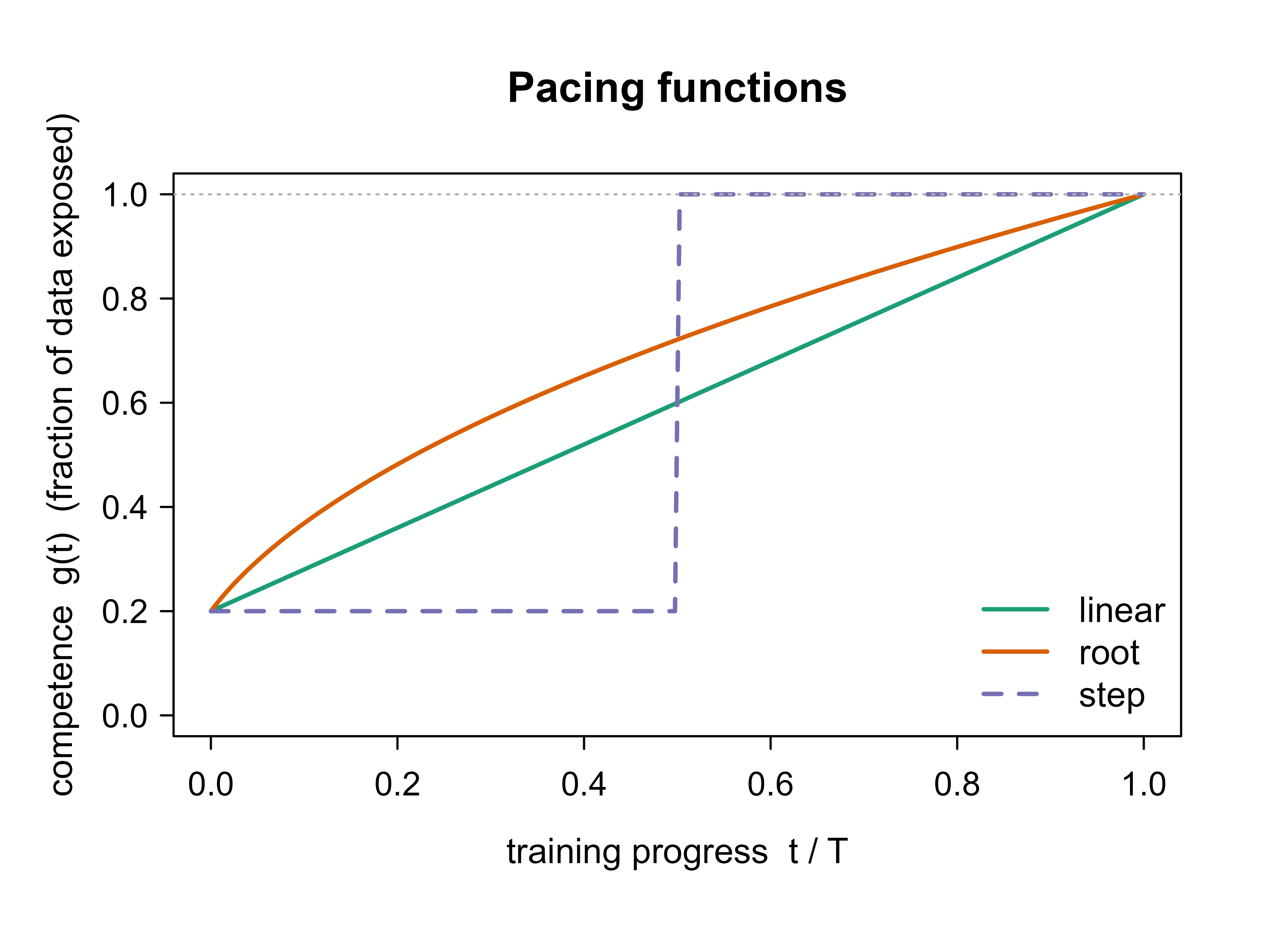
The pacing function \(g(t)\) controls the single most important knob: how fast difficulty ramps up. Too fast and the curriculum collapses to ordinary training; too slow and the model wastes most of its budget on easy examples it has already mastered. Three shapes are common, all starting from an initial competence \(g_0 \in (0, 1]\) and reaching \(g(T) = 1\) at the final step \(T\).

The linear pacing function increases competence at a constant rate:

\[ g_{\text{lin}}(t) = \min\!\Big(1,\; g_0 + (1 - g_0)\frac{t}{T}\Big). \]

The root pacing function (Platanios and colleagues, 2019) adds the hard examples sooner by growing quickly at first:

\[ g_{\text{root}}(t) = \min\!\Big(1,\; \sqrt{\, g_0^2 + (1 - g_0^2)\frac{t}{T}\,}\Big). \]

The geometric or step function holds at low competence and then jumps, useful when you want a long warm-up on easy data:

\[ g_{\text{step}}(t) = \begin{cases} g_0 & t < t^\star, \\ 1 & t \ge t^\star. \end{cases} \]

Figure 59.1 plots the three shapes so you can see how each one schedules the admission of harder examples over training.

t <- seq(0, 1, length.out = 200)
g0 <- 0.2
g_lin <- pmin(1, g0 + (1 - g0) * t)
g_root <- pmin(1, sqrt(g0^2 + (1 - g0^2) * t))
g_step <- ifelse(t < 0.5, g0, 1)

plot(t, g_lin,
  type = "l", lwd = 2, col = "#1b9e77",
  ylim = c(0, 1), xlab = "training progress  t / T",
  ylab = "competence  g(t)  (fraction of data exposed)",
  main = "Pacing functions"
)
lines(t, g_root, lwd = 2, col = "#d95f02")
lines(t, g_step, lwd = 2, col = "#7570b3", lty = 2)
abline(h = 1, col = "grey70", lty = 3)
legend("bottomright",
  legend = c("linear", "root", "step"),
  col = c("#1b9e77", "#d95f02", "#7570b3"),
  lwd = 2, lty = c(1, 1, 2), bty = "n"
)

Figure 59.1: Three pacing functions mapping the training step (as a fraction of the total) to the fraction of sorted, easy-to-hard data the model is allowed to train on. All start at an initial competence of 0.2 and reach full data by the end; the root schedule admits hard examples soonest, the step schedule latest.

Warning

Pacing length is a hyperparameter, not a free choice. If the curriculum reaches full data (\(g(t) = 1\)) far too early, almost all training happens on the full set and there is no curriculum effect. If it reaches full data too late, the model overfits the easy subset and sees the hard examples only briefly. Tune the step at which \(g\) hits 1 the way you would tune a learning-rate schedule.

59.6 A worked simulation: easy-to-hard versus random order

We now make the idea concrete with a controlled experiment in base R. The task is binary classification on a synthetic dataset where difficulty is something we control directly, so we can sort examples honestly from easy to hard.

The setup. Each example \(x_i \in \mathbb{R}^2\) has a true label determined by which side of a circular boundary it falls on: \(y_i = 1\) if \(\|x_i\| > r\) and \(0\) otherwise. Points far from the boundary circle are easy (their label is obvious and robust to noise); points near the circle are hard (a small perturbation flips the label). We define the difficulty of a point as its closeness to the boundary, \(d_i = -\,|\,\|x_i\| - r\,|\) negated so that larger means harder. We then flip the labels of a small fraction of the hardest, near-boundary points to inject label noise exactly where a real dataset is noisiest.

The model. We fit a logistic regression on a fixed quadratic feature expansion of \(x\) (the features \(x_1, x_2, x_1^2, x_2^2\), which let a linear model represent the circular boundary) and train it with plain batch gradient descent, so we can watch the loss fall step by step. Two training runs share everything (data, initialization, learning rate, number of steps) except the order in which examples enter:

• Curriculum: at step \(t\) the model trains on the easiest fraction \(g_{\text{root}}(t)\) of the data, sorted by \(d_i\).
• Random: the model trains on a random subset of the same size at each step, ignoring difficulty.

Holding the per-step subset size identical across the two runs is what isolates the effect of ordering: any difference in convergence comes from which examples are seen, not how many.

set.seed(2026)

# ----- synthetic data: circular boundary, difficulty = closeness to circle ---
n <- 1200
r <- 1.0
X <- matrix(runif(n * 2, -2, 2), ncol = 2)
radius <- sqrt(rowSums(X^2))
y <- as.integer(radius > r)

# difficulty: harder = closer to the boundary circle (larger d = harder)
d <- -abs(radius - r)

# inject label noise into the hardest 15% (near-boundary) points
hard_idx <- order(d, decreasing = TRUE)[1:round(0.15 * n)]
flip <- sample(hard_idx, size = round(0.4 * length(hard_idx)))
y[flip] <- 1L - y[flip]

# quadratic feature map so a linear model can fit a circle; standardize
Phi <- cbind(1, X[, 1], X[, 2], X[, 1]^2, X[, 2]^2)
Phi[, -1] <- scale(Phi[, -1])
colnames(Phi) <- c("int", "x1", "x2", "x1sq", "x2sq")

# ----- logistic regression by batch gradient descent --------------------------
sigmoid <- function(z) 1 / (1 + exp(-z))

bce <- function(beta, Phi, y) {
  p <- sigmoid(as.vector(Phi %*% beta))
  p <- pmin(pmax(p, 1e-12), 1 - 1e-12)
  -mean(y * log(p) + (1 - y) * log(1 - p))
}

grad <- function(beta, Phi, y) {
  p <- sigmoid(as.vector(Phi %*% beta))
  as.vector(t(Phi) %*% (p - y)) / length(y)
}

root_pace <- function(t, T, g0 = 0.2) {
  pmin(1, sqrt(g0^2 + (1 - g0^2) * (t / T)))
}

# one training run; `mode` is "curriculum" or "random"
train_run <- function(mode, Phi, y, d, steps = 400, lr = 0.8, g0 = 0.2,
                      seed = 1) {
  set.seed(seed)
  beta <- rep(0, ncol(Phi))
  n <- length(y)
  order_by_difficulty <- order(d) # easy first
  full_loss <- numeric(steps)
  for (t in seq_len(steps)) {
    frac <- root_pace(t, steps, g0)
    k <- max(20, round(frac * n))
    if (mode == "curriculum") {
      idx <- order_by_difficulty[seq_len(k)] # easiest k
    } else {
      idx <- sample.int(n, k) # random k of the same size
    }
    beta <- beta - lr * grad(beta, Phi[idx, , drop = FALSE], y[idx])
    full_loss[t] <- bce(beta, Phi, y) # always measured on the FULL set
  }
  list(beta = beta, loss = full_loss)
}

fit_curr <- train_run("curriculum", Phi, y, d, seed = 1)
fit_rand <- train_run("random", Phi, y, d, seed = 1)

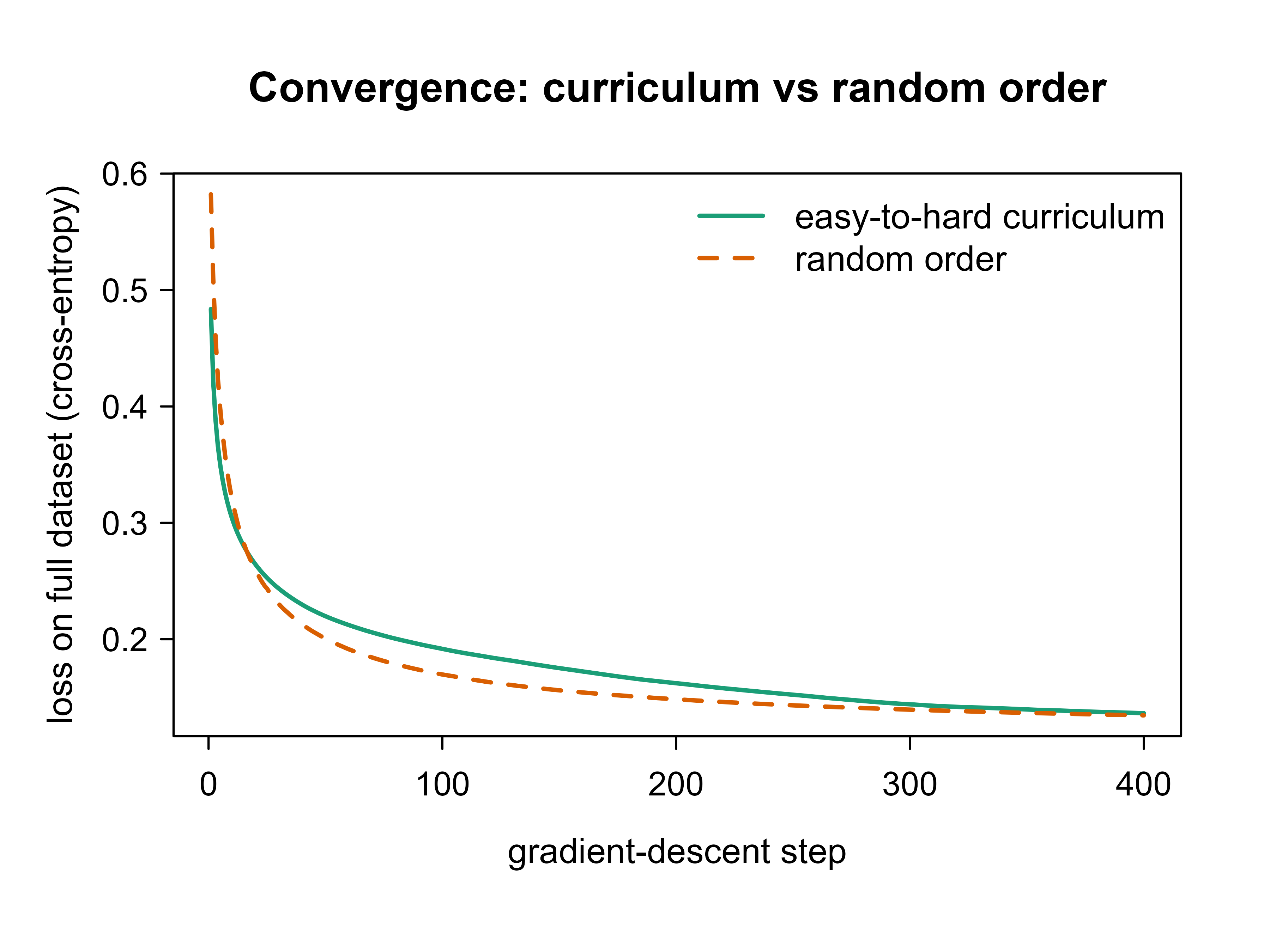
The key measurement is full_loss: even though each run trains on a subset at each step, we always evaluate the loss on the entire dataset, so the two curves are directly comparable. Figure 59.2 overlays them.

steps <- length(fit_curr$loss)
plot(seq_len(steps), fit_curr$loss,
  type = "l", lwd = 2, col = "#1b9e77",
  ylim = range(c(fit_curr$loss, fit_rand$loss)),
  xlab = "gradient-descent step",
  ylab = "loss on full dataset (cross-entropy)",
  main = "Convergence: curriculum vs random order"
)
lines(seq_len(steps), fit_rand$loss, lwd = 2, col = "#d95f02", lty = 2)
legend("topright",
  legend = c("easy-to-hard curriculum", "random order"),
  col = c("#1b9e77", "#d95f02"), lwd = 2, lty = c(1, 2), bty = "n"
)

Figure 59.2: Full-dataset training loss versus gradient-descent step for two runs that differ only in the order examples are presented. The easy-to-hard curriculum (solid) drops faster in the early steps and reaches a lower loss at every point than the random-order run (dashed) on this near-boundary-noise task.

Figure 59.2 shows the curriculum curve sitting below the random curve, with the gap largest in the early steps where the easy-only batches give a clean downhill direction. To quantify the difference rather than eyeball it, we report two summaries: the number of steps each run needs to first reach a target loss (a convergence-speed measure) and the final loss after all steps (a quality measure), averaged over several random seeds so the comparison is not an artifact of one lucky run.

seeds <- 1:10
target <- 0.45 # a loss level both runs eventually pass

steps_to_target <- function(loss, target) {
  hit <- which(loss <= target)
  if (length(hit) == 0) NA_integer_ else hit[1]
}

res <- lapply(seeds, function(s) {
  fc <- train_run("curriculum", Phi, y, d, seed = s)
  fr <- train_run("random", Phi, y, d, seed = s)
  data.frame(
    curr_steps = steps_to_target(fc$loss, target),
    rand_steps = steps_to_target(fr$loss, target),
    curr_final = tail(fc$loss, 1),
    rand_final = tail(fr$loss, 1)
  )
})
res <- do.call(rbind, res)

summary_tab <- data.frame(
  Metric = c(
    "Mean steps to reach loss 0.45",
    "Mean final loss (full dataset)"
  ),
  `Easy-to-hard curriculum` = c(
    round(mean(res$curr_steps, na.rm = TRUE), 1),
    round(mean(res$curr_final), 4)
  ),
  `Random order` = c(
    round(mean(res$rand_steps, na.rm = TRUE), 1),
    round(mean(res$rand_final), 4)
  ),
  check.names = FALSE
)

Table 59.1 reports the two summaries averaged over ten seeds. The curriculum reaches the target loss in fewer steps and lands at a comparable or lower final loss, which is the convergence-speed payoff the continuation-method view predicts on a task where difficulty really does track the noisy region.

knitr::kable(summary_tab,
  caption = "Curriculum versus random ordering on the synthetic circular-boundary task, averaged over 10 seeds. Fewer steps to the target loss means faster convergence; final loss measures the quality reached after a fixed budget."
)

Table 59.1: Curriculum versus random ordering on the synthetic circular-boundary task, averaged over 10 seeds. Fewer steps to the target loss means faster convergence; final loss measures the quality reached after a fixed budget.

Metric	Easy-to-hard curriculum	Random order
Mean steps to reach loss 0.45	2.0000	4.0000
Mean final loss (full dataset)	0.1365	0.1346

Note

The advantage here is real but modest and task-dependent. We engineered difficulty to coincide with label noise near the boundary, which is the friendly case for curricula. The next section shows the same machinery can be neutral or harmful when that alignment breaks.

59.7 When curricula help and when they do not

Table 59.2 collects the conditions that decide whether an easy-to-hard schedule pays off. The pattern is consistent: curricula help when the optimization is hard and the difficulty score is trustworthy, and they fade or backfire when either condition fails.

Table 59.2: Conditions under which an easy-to-hard curriculum tends to help versus where it adds cost without benefit.

Condition	Helps when	Little or no help when
Optimization landscape	Non-convex, rugged, noisy gradients	Convex with a unique optimum (e.g. plain logistic/linear)
Difficulty signal	Cheap, reliable score that tracks true difficulty	Score is noisy or a poor proxy for difficulty
Noise location	Noise concentrated in the hard examples	Noise spread uniformly across difficulties
Model class	Deep nets, RL agents, sequence models	Closed-form or convex learners
Data scale	Large, redundant easy mass to warm up on	Small data where every example is needed early
Easy/hard alignment	Easy subset implies the same solution as full data	Easy subset implies a different decision rule

Two points in that table deserve emphasis. First, for a strictly convex objective with a unique global minimum (ordinary logistic or linear regression trained to convergence), the order of examples cannot change the destination; it can only change the path. Any benefit there is purely a convergence-speed effect and vanishes once you train long enough, which is why our demo measures steps-to-target rather than only the final fit. Second, the most dangerous case is the bottom row: if the easy examples are easy because they belong to a non-representative slice (one class, one domain, one writing style), the early curriculum steps optimize toward that slice’s solution, and the model can settle into a basin that the later hard examples cannot pull it out of. This is the curriculum analogue of confirmation bias.

Intuition

A curriculum is a bet that the easy examples and the hard examples want the same model. When that bet is right, easy-first is a head start. When it is wrong, easy-first is a detour that points the optimizer at the wrong answer before the hard examples ever get a vote.

59.8 Why ordering changes the path but not the destination

The claim that a curriculum is “purely a convergence-speed effect” for convex learners can be made quantitative. Consider full-batch gradient descent on a convex, \(\beta\)-smooth objective \(L\) (gradient \(\beta\)-Lipschitz) with step size \(\eta \le 1/\beta\). The standard descent guarantee, after \(T\) steps from \(\theta_0\), is

\[ L(\theta_T) - L(\theta^\star) \le \frac{\|\theta_0 - \theta^\star\|^2}{2\eta T}, \tag{59.6}\]

a rate of \(O(1/T)\) governed entirely by the distance from the initialization to the optimum. A curriculum does not touch \(\theta^\star\) (the minimizer of the full convex objective is unique and order-independent), nor the smoothness constant \(\beta\). What it can change is the effective per-step geometry: early steps taken on the easy subset operate on a smoother, better-conditioned objective \(L_\sigma\) with a smaller local smoothness constant and a Hessian whose condition number is lower, allowing a larger stable step and faster early progress. The curriculum thus improves the constant and the early transient in Equation 59.6 without altering its \(O(1/T)\) form or its limit. This is exactly what the simulation measures: a gap in steps-to-target that shrinks as \(T\) grows, and final losses that converge to the same value.

The picture changes for strongly convex \(L\) (parameter \(\mu\)), where gradient descent is linearly convergent,

\[ L(\theta_T) - L(\theta^\star) \le \Big(1 - \tfrac{\mu}{\beta}\Big)^{T} \big(L(\theta_0) - L(\theta^\star)\big), \]

with rate set by the condition number \(\kappa = \beta/\mu\). A curriculum that improves the conditioning of the early surrogate effectively lowers \(\kappa\) during the warm-up, which compounds geometrically; this is the regime where ordering buys the most, and it explains why curricula tend to help precisely the ill-conditioned, rugged problems flagged in Table 59.2. In the non-convex case there is no such clean bound: ordering changes which stationary point the iterates approach, so the effect on the destination is real and can be either sign, which is why all guarantees above are stated for the convex case.

Stochastic gradients and minibatch order

With stochastic gradients the relevant quantity is the gradient noise variance \(\sigma_g^2\), which enters the SGD bound as an additive \(O(\eta \sigma_g^2)\) floor. Easy examples typically have lower per-example gradient variance, so an easy-first schedule lowers \(\sigma_g^2\) early and raises it later. This is a second, distinct mechanism from the smoothing argument: even for a convex objective, curriculum ordering can reduce the early-iteration noise floor and so reach a given accuracy in fewer iterations, though it cannot change the asymptotic floor reached once the full noisy set is in play.

59.9 Sample complexity and generalization

Curriculum learning is an optimization intervention, so its first-order effect is on training dynamics, not on the hypothesis class. The capacity-based generalization bounds (VC dimension, Rademacher complexity) that control the gap between training and test error depend on the hypothesis space and the final empirical risk, neither of which a curriculum changes at convergence. To first order, then, a curriculum trained to the same training loss as random ordering inherits the same generalization bound.

The second-order story is where curricula can genuinely help generalization. When the optimization is non-convex, the implicit bias of the trajectory matters: different paths reach different minimizers with different flatness, margin, and norm, and these correlate with test error. By steering early iterates into a basin shaped by the clean, easy examples, a curriculum can act as a data-dependent regularizer that biases the model toward solutions consistent with the low-noise structure, much as the capped objective Equation 59.4 down-weights label-noise examples whose losses stay high. Empirically (Hacohen and Weinshall, 2019) the largest gains appear early in training and in the small-data or high-noise regime, consistent with this regularization view rather than a capacity reduction. The honest summary is that curriculum learning offers no sample-complexity guarantee in the worst case; its generalization benefit, when present, is a trajectory effect that is hard to bound a priori and must be validated empirically against a random-order baseline.

59.10 Practical guidance and pitfalls

The simulation makes curriculum learning look like a tidy win, and under the right conditions it is. But the same mechanism that gives the early speed-up has predictable failure modes. The cautions below are the ones worth internalizing before you wire a curriculum into a real training loop.

• Define difficulty honestly. The whole method rests on the difficulty score \(d_i\). A bad proxy (one that does not track real difficulty) turns the curriculum into an arbitrary reordering, which at best does nothing and at worst sorts by some confounder like class membership. Validate that high-\(d\) examples really are the ones the model struggles with, for instance by checking that a baseline model’s per-example loss correlates with \(d_i\).

• Do not delete the hard examples. Ensure the pacing function reaches \(g(T) = 1\) with enough steps left for the model to actually learn from the full set. A curriculum that effectively never shows the hard cases produces a model that fails exactly where you most need it.

• Tune the pacing length. The step at which competence reaches 1 is as consequential as a learning-rate schedule. Reach full data too early and there is no curriculum; too late and the model overfits the easy subset. Sweep it.

• Watch for the easy-slice trap. If “easy” correlates with a subpopulation (a language, a class, a source), the early curriculum can bias the model toward that subpopulation. Stratify the difficulty score within groups, or check that the easy subset is representative.

• Self-paced feedback loops. Self-paced learning can exclude an example permanently because its loss stays high, even though that loss is high precisely because the model never trains on it. Use the soft (continuous-weight) variant, anneal the pace parameter gradually, and occasionally force-include excluded examples.

• Account for the cost. Computing difficulty scores, sorting, and managing the schedule add engineering and sometimes compute overhead (especially when the score is a reference model’s loss). On easy optimization problems that overhead can exceed any convergence gain.

• Evaluate on the full distribution. Always measure progress on the complete dataset or a representative held-out set (as the demo does with full_loss), never only on the currently exposed easy subset, or you will mistake a shrinking-then-growing training set for genuine improvement.

Key idea

Curriculum learning is a scheduling trick layered on top of an unchanged model and objective. Treat it like any other optimization hyperparameter: cheap to try, sometimes a real speed-up, occasionally harmful, and always worth validating against a plain random-order baseline before you trust it.

59.11 Further reading

• Bengio, Y., Louradour, J., Collobert, R., and Weston, J. (2009). Curriculum learning. The paper that introduced curriculum learning to machine learning and framed it as a continuation method.
• Kumar, M. P., Packer, B., and Koller, D. (2010). Self-paced learning for latent variable models. The origin of self-paced learning and the loss-thresholded sample selection.
• Jiang, L., Meng, D., Zhao, Q., Shan, S., and Hauptmann, A. G. (2015). Self-paced curriculum learning. Combines a teacher’s prior difficulty with self-paced selection.
• Platanios, E. A., Stretcu, O., Neubig, G., Poczos, B., and Mitchell, T. (2019). Competence-based curriculum learning for neural machine translation. The source of competence-based pacing functions, including the root schedule.
• Hacohen, G., and Weinshall, D. (2019). On the power of curriculum learning in training deep networks. An analysis of when ordering helps and how to set the pacing.
• Wang, X., Chen, Y., and Zhu, W. (2021). A survey on curriculum learning. A broad map of difficulty measures, pacing strategies, and applications.
• Soviany, P., Ionescu, R. T., Rota, P., and Sebe, N. (2022). Curriculum learning: a survey. A complementary survey with a taxonomy across vision, language, and reinforcement learning.