44  Graph Neural Networks

Most models in this book assume that observations are independent rows in a table. Each row carries its own features, and the model maps those features to a target. Many problems do not fit that picture. A user in a social network is described partly by who their friends are. A molecule’s properties depend on how its atoms are bonded. A transaction looks normal in isolation but suspicious once you see the accounts it connects to. In these settings the relationships between observations carry as much signal as the observations themselves.

Graph Neural Networks (GNNs) are models that learn from data structured as a graph: a set of nodes (entities) connected by edges (relationships).¹ The core idea is that a node’s representation should be built from its own features plus information gathered from its neighbors. Stack a few rounds of this neighbor gathering and each node sees a widening region of the graph. This chapter develops the math of message passing, walks through the three architectures a practitioner meets first (GCN, GraphSAGE, GAT), implements one graph convolution layer in base R so the mechanics are concrete, and gives practical guidance including the over-smoothing failure mode.

Intuition

Picture each node passing notes to its neighbors. In one round, you learn what your immediate friends know. In a second round, your friends have already absorbed what their friends know, so a piece of that reaches you too. A GNN is just this rumor-spreading process made differentiable, so the rules for what to pass and how to combine it can be learned from data.

What you will learn

how to represent a graph as matrices, the single message-passing template that nearly every GNN layer follows, how GCN, GraphSAGE, and GAT each fill in that template, how to build a graph convolution by hand in base R, and the practical traps (over-smoothing, heterophily, scale) that separate a working GNN from a broken one.

44.1 Where GNNs Fit in a Modern Workflow

In an applied ML or AI pipeline, GNNs occupy the slot you reach for when the relational structure is part of the data, not an afterthought. Typical entry points:

• Fraud and risk: accounts, devices, and transactions form a graph; fraud rings show up as suspicious subgraphs.
• Recommendation: users and items form a bipartite graph; predicting a missing edge is the recommendation (Chapter 89).
• Molecules and materials: atoms are nodes, bonds are edges, and the task is to predict a property of the whole graph.
• Knowledge graphs and retrieval: entities and relations support link prediction and graph-aware retrieval that can feed a downstream LLM (Chapter 40).
• Traffic, supply chains, and infrastructure: sensors and roads or warehouses and routes form a graph evolving over time.

A reasonable rule of thumb: if you can draw your data as nodes and edges and you believe a node’s label depends on its neighborhood, a GNN is worth trying. If the relationships are weak or absent, a plain tabular model (gradient boosting (Chapter 12), a feedforward network (Chapter 15)) is usually simpler and stronger. GNNs are not a replacement for those models; they are the relational extension of them.

When to use this

reach for a GNN when the edges carry signal you would otherwise have to engineer by hand (counts of suspicious neighbors, average rating of co-purchased items, and so on). The GNN learns those neighborhood summaries for you. When the edges are noise or convenience, skip it.

44.2 Graphs and Adjacency

A graph is \(G = (V, E)\) with node set \(V\) of size \(n = |V|\) and edge set \(E\). We store node features in a matrix \(X \in \mathbb{R}^{n \times d}\), where row \(i\) is the feature vector \(x_i\) of node \(i\) and \(d\) is the number of input features.

The connectivity is encoded in the adjacency matrix \(A \in \mathbb{R}^{n \times n}\):

\[ A_{ij} = \begin{cases} 1 & \text{if there is an edge from } i \text{ to } j \\ 0 & \text{otherwise} \end{cases} \]

For an undirected graph \(A\) is symmetric, \(A = A^\top\). Weighted graphs replace the \(1\) with an edge weight. The degree of node \(i\) is the number of its neighbors, \(\deg(i) = \sum_j A_{ij}\), and the diagonal degree matrix \(D\) has \(D_{ii} = \deg(i)\) and zeros off the diagonal.

Two derived matrices appear constantly. The combinatorial graph Laplacian is

\[ L = D - A, \]

and its symmetric normalized form is

\[ L_{\text{sym}} = I - D^{-1/2} A D^{-1/2}. \]

The Laplacian measures how much a signal on the graph varies between connected nodes, and it is the bridge between GNNs and classical spectral graph theory.²

Note

You do not need spectral graph theory to use a GNN, but it explains why the normalization in the GCN layer below looks the way it does. We flag the connection and move on; the message-passing view in the next section is self-contained.

Before choosing an architecture, decide what you are predicting. Tasks on graphs come in three flavors, and the distinction drives everything downstream, from how you split the data to what the final layer outputs. Table 44.1 summarizes the three task levels and what each one produces.

Table 44.1: The three levels of prediction task on graphs, with an example and the output shape for each.

Task level	What you predict	Example	Output shape
Node	a label per node	which users are bots	one prediction per node
Edge	whether or how two nodes link	will user \(u\) buy item \(v\)	one prediction per node pair
Graph	a label for the whole graph	is this molecule toxic	one prediction per graph

44.3 Message Passing: The Common Framework

Almost every GNN layer is an instance of one pattern. Each node updates its representation by (1) collecting messages from its neighbors, (2) aggregating those messages into a single vector, and (3) combining the aggregate with its own current state. Let \(h_i^{(k)}\) denote the representation of node \(i\) after layer \(k\), with \(h_i^{(0)} = x_i\). Let \(\mathcal{N}(i)\) be the neighbors of \(i\). Then

\[ m_i^{(k)} = \underset{j \in \mathcal{N}(i)}{\text{AGGREGATE}} \left( \phi\!\left(h_i^{(k-1)}, h_j^{(k-1)}\right) \right), \]

\[ h_i^{(k)} = \text{UPDATE}\!\left(h_i^{(k-1)}, m_i^{(k)}\right). \tag{44.1}\]

Here \(\phi\) builds a message from a node and one of its neighbors, AGGREGATE is a permutation-invariant pooling function (sum, mean, or max, because neighbors have no inherent order), and UPDATE merges the pooled message with the node’s prior state, usually through a learned linear map and a nonlinearity.

Key idea

AGGREGATE must be permutation invariant, meaning the answer cannot depend on the order you list the neighbors in. A node’s neighbors form a set, not a sequence, so the only legal operations are ones like sum, mean, and max that ignore order. This single constraint is what distinguishes a GNN from feeding a node’s neighbor list into an ordinary network.

The depth \(k\) controls the receptive field. After \(k\) layers, node \(i\)’s representation depends on every node within \(k\) hops. This is the graph analogue of a convolutional network’s growing receptive field over an image. The architectures below differ only in their choices of \(\phi\), AGGREGATE, and UPDATE, so once you have this template the differences between GCN, GraphSAGE, and GAT are small and easy to keep straight.

44.4 Graph Convolutional Network (GCN)

The GCN layer of Kipf and Welling (2017) is the most common starting point. Its propagation rule for a full layer is

\[ H^{(k)} = \sigma\!\left( \hat{A}\, H^{(k-1)} W^{(k)} \right), \]

where \(H^{(k-1)} \in \mathbb{R}^{n \times d_{k-1}}\) is the matrix of node representations entering the layer, \(W^{(k)} \in \mathbb{R}^{d_{k-1} \times d_k}\) is a learnable weight matrix, \(\sigma\) is an elementwise nonlinearity such as ReLU, and \(\hat{A}\) is the symmetric normalized adjacency with self-loops.

The matrix \(\hat{A}\) is built in two steps. First add self-loops so each node keeps its own information,

\[ \tilde{A} = A + I, \]

with degree matrix \(\tilde{D}\) where \(\tilde{D}_{ii} = \sum_j \tilde{A}_{ij}\). Then normalize symmetrically,

\[ \hat{A} = \tilde{D}^{-1/2}\, \tilde{A}\, \tilde{D}^{-1/2}. \]

Why this normalization? The product \(\tilde{A} H\) alone is a sum over neighbors, so high-degree nodes would accumulate large magnitudes and dominate. Dividing by degrees rebalances this. The symmetric form \(\tilde{D}^{-1/2} \tilde{A} \tilde{D}^{-1/2}\) scales entry \((i,j)\) by \(1 / \sqrt{\deg(i)\,\deg(j)}\), which keeps the operator’s spectrum bounded and stabilizes training. In message-passing terms, GCN uses a degree-weighted mean as AGGREGATE, a shared linear map as the message and update, and folds the node’s own state in through the self-loop.

Warning

If you forget the self-loop in \(\tilde{A} = A + I\), each node throws away its own features and is described purely by its neighbors. This silently degrades accuracy and is one of the most common GNN implementation bugs. Always add self-loops before normalizing.

GCN is simple and fast, but the same weight matrix \(W^{(k)}\) and the fixed normalization apply everywhere, so the model cannot weight some neighbors more than others, and it needs the whole adjacency matrix at training time (it is transductive in its basic form).³

44.4.1 Derivation: From Spectral Convolution to the GCN Layer

The GCN rule is not arbitrary. It is a first-order approximation of a spectral graph convolution, and tracing that derivation explains every term in \(\hat A H W\). Work with the symmetric normalized Laplacian \(L_{\text{sym}} = I - D^{-1/2} A D^{-1/2}\), which is real symmetric and positive semidefinite, hence admits an eigendecomposition

\[ L_{\text{sym}} = U \Lambda U^\top, \qquad \Lambda = \operatorname{diag}(\lambda_1, \dots, \lambda_n), \quad 0 = \lambda_1 \le \dots \le \lambda_n \le 2 . \tag{44.2}\]

The bound \(\lambda_n \le 2\) is standard for \(L_{\text{sym}}\) and is the fact that makes the approximation below stable. The graph Fourier transform of a signal \(x \in \mathbb{R}^n\) (one scalar feature per node) is \(\hat x = U^\top x\), and a spectral filter with frequency response \(g_\theta(\Lambda)\) acts as

\[ g_\theta \star x = U\, g_\theta(\Lambda)\, U^\top x . \tag{44.3}\]

Evaluating \(U g_\theta(\Lambda) U^\top\) requires the full eigendecomposition, an \(O(n^3)\) cost, and the filter has \(n\) free parameters, so it is neither scalable nor localized. Defferrard, Bresson, and Vandergheynst (2016) make the filter a degree-\(K\) polynomial in \(\Lambda\) expanded in Chebyshev polynomials \(T_k\),

\[ g_\theta(\Lambda) \approx \sum_{k=0}^{K} \theta_k\, T_k(\tilde\Lambda), \qquad \tilde\Lambda = \tfrac{2}{\lambda_n}\Lambda - I , \tag{44.4}\]

where the rescaling sends the spectrum into \([-1,1]\), the domain on which \(T_k\) are defined by the recurrence \(T_0 = 1\), \(T_1 = z\), \(T_k(z) = 2 z\, T_{k-1}(z) - T_{k-2}(z)\). Because \(U T_k(\tilde\Lambda) U^\top = T_k(\tilde L)\) with \(\tilde L = \tfrac{2}{\lambda_n} L_{\text{sym}} - I\), the filter becomes a polynomial in the Laplacian itself,

\[ g_\theta \star x \approx \sum_{k=0}^{K} \theta_k\, T_k(\tilde L)\, x , \tag{44.5}\]

which costs \(O(K |E|)\) via sparse matrix-vector products and is exactly \(K\)-localized: \(T_k(\tilde L)\) has the same sparsity pattern as \(L^k\), so it touches only nodes within \(k\) hops. This is already a usable GNN (ChebNet). Kipf and Welling specialize it twice. First set \(K = 1\), keeping only the constant and linear terms, and approximate \(\lambda_n \approx 2\) so that \(\tilde L = L_{\text{sym}} - I = -D^{-1/2} A D^{-1/2}\). Then Equation 44.5 collapses to

\[ g_\theta \star x \approx \theta_0\, x + \theta_1 \big( L_{\text{sym}} - I \big) x = \theta_0\, x - \theta_1\, D^{-1/2} A D^{-1/2} x . \tag{44.6}\]

Second, tie the two parameters by \(\theta = \theta_0 = -\theta_1\) (a regularization that halves the parameter count and discourages overfitting), giving the single-parameter filter

\[ g_\theta \star x \approx \theta \big( I + D^{-1/2} A D^{-1/2} \big) x . \tag{44.7}\]

The operator \(I + D^{-1/2} A D^{-1/2}\) has eigenvalues in \([0, 2]\) (since those of \(D^{-1/2} A D^{-1/2}\) lie in \([-1,1]\)). Stacking many layers each multiplying by such an operator would amplify signals and cause numerical instability, so Kipf and Welling apply the renormalization trick: replace \(I + D^{-1/2} A D^{-1/2}\) by \(\tilde D^{-1/2} \tilde A \tilde D^{-1/2}\) with \(\tilde A = A + I\) and \(\tilde D_{ii} = \sum_j \tilde A_{ij}\). This is exactly the \(\hat A\) defined above; it folds the identity (the self-loop) directly into the adjacency before normalizing, which keeps the spectrum bounded in a way that is stable under repeated application. Promoting the scalar feature to a \(d\)-dimensional one (so \(x\) becomes \(H \in \mathbb{R}^{n \times d}\)) and the scalar \(\theta\) to a weight matrix \(W\) yields the layer pre-activation \(\hat A H W\), and applying a nonlinearity gives Equation 44.6’s matured form, the GCN propagation rule. Every piece, the self-loop, the symmetric normalization, the linear map, is now accounted for by this chain of approximations rather than asserted.

Note

The renormalization trick is more than cosmetic. The naive operator \(I + D^{-1/2} A D^{-1/2}\) has top eigenvalue \(2\), so \(L\) stacked layers scale the leading graph-frequency component by up to \(2^L\). The renormalized \(\hat A\) has spectral radius at most \(1\), which is what permits stacking several layers without exploding activations. It also shifts the spectrum so that the all-ones (constant) signal is the dominant eigenvector, which is the seed of over-smoothing analyzed below.

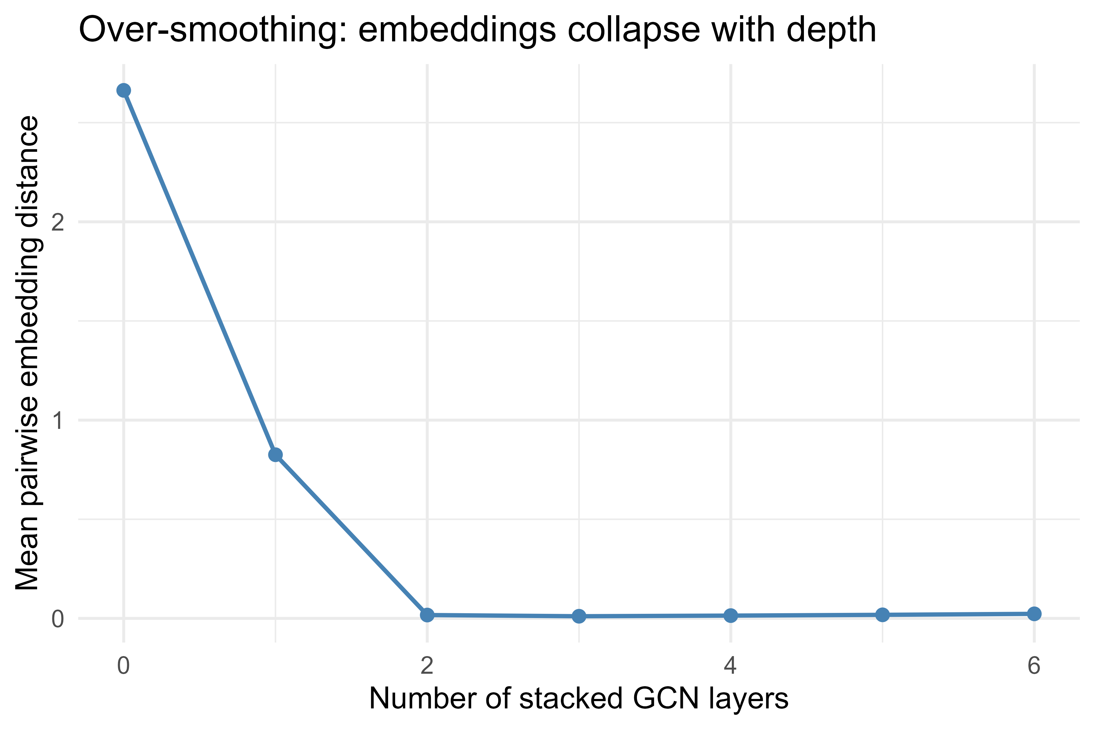
44.4.2 Over-smoothing as Convergence to the Dominant Eigenvector

The collapse seen in Figure 44.1 is not a coincidence of the random weights; it is forced by the spectrum of \(\hat A\). Strip away the nonlinearity and the per-layer weights for a moment (the linear case already captures the mechanism). After \(k\) layers the embeddings are \(H^{(k)} = \hat A^{k} X W^{(1)} \cdots W^{(k)}\), so the question reduces to the behavior of \(\hat A^{k}\) as \(k \to \infty\). Write the eigendecomposition \(\hat A = \sum_{r=1}^{n} \mu_r\, u_r u_r^\top\) with \(|\mu_1| \ge |\mu_2| \ge \dots\). For a connected non-bipartite graph the symmetric normalized adjacency with self-loops has a unique top eigenvalue \(\mu_1 = 1\) with eigenvector

\[ u_1 \propto \tilde D^{1/2} \mathbf{1}, \qquad (u_1)_i \propto \sqrt{\tilde d_i} , \tag{44.8}\]

and all other eigenvalues satisfy \(|\mu_r| < 1\). Decomposing any feature column \(x = \sum_r c_r u_r\) gives

\[ \hat A^{k} x = \sum_{r=1}^{n} \mu_r^{k}\, c_r\, u_r = c_1\, u_1 + \sum_{r \ge 2} \mu_r^{k}\, c_r\, u_r \xrightarrow{k \to \infty} c_1\, u_1 , \tag{44.9}\]

because every term with \(r \ge 2\) decays geometrically at rate \(|\mu_r|^k\). The limit \(c_1 u_1\) is the same for every node up to its \(\sqrt{\tilde d_i}\) scaling: all nodes collapse onto a single direction whose entries depend only on degree, erasing the feature information a classifier needs. The convergence rate is governed by the spectral gap \(1 - |\mu_2|\): the residual distance from the limit shrinks like \(|\mu_2|^k\), so well-connected graphs (large gap) over-smooth in very few layers, exactly the two-to-three-layer collapse the figure shows. The ReLU and the weights modulate the constants but do not change the geometric decay of the non-dominant components, which is why over-smoothing is robust to the details of the network. This also clarifies why the mitigations listed below work: residual connections add back a component along the original \(x\) that \(\hat A^k\) would otherwise annihilate, and jumping knowledge reads off the shallow layers before the high-frequency components have decayed.

Tip

The diagnostic in Figure 44.1 measures mean pairwise embedding distance, which is a direct estimate of the energy in the non-dominant eigencomponents. Plotting it on a log scale against depth should give an approximately straight line whose slope estimates \(\log |\mu_2|\), the second-largest eigenvalue magnitude of \(\hat A\). That slope is a quantitative read on how aggressively your particular graph will over-smooth.

We can verify Equation 44.8 and Equation 44.9 directly. The top eigenvalue of \(\hat A\) should equal \(1\), its eigenvector should be proportional to \(\sqrt{\tilde d_i}\), and iterating \(\hat A^k x\) should align with that eigenvector at a rate set by \(|\mu_2|\).

# Build the same 6-node two-cluster graph and symmetric-normalized adjacency
# that the base-R GCN section below uses, so this check is self-contained.
A <- matrix(0, 6, 6)
for (e in list(c(1, 2), c(1, 3), c(2, 3), c(4, 5), c(4, 6), c(5, 6), c(3, 4))) {
  A[e[1], e[2]] <- 1; A[e[2], e[1]] <- 1
}
gcn_norm <- function(A) {
  At <- A + diag(nrow(A)); d <- rowSums(At)
  diag(1 / sqrt(d)) %*% At %*% diag(1 / sqrt(d))
}
Ahat  <- gcn_norm(A)
eig   <- eigen(Ahat, symmetric = TRUE)
mu1   <- eig$values[1]              # should be 1
mu2   <- abs(eig$values[2])        # spectral-gap term
u1    <- abs(eig$vectors[, 1])     # dominant eigenvector (sign-free)

deg_self <- rowSums(A + diag(nrow(A)))   # tilde-degrees
# u1 should be proportional to sqrt(tilde d): check correlation is ~1
cor_check <- cor(u1, sqrt(deg_self))

# Power iteration: cosine of angle between Ahat^k x and u1 should -> 1.
# Rate is set by |mu2|, so on a small graph it takes a few dozen steps.
cos_align <- function(a, b) abs(sum(a * b)) / (sqrt(sum(a^2)) * sqrt(sum(b^2)))
v <- rnorm(nrow(A))
align <- numeric(40)
for (k in 1:40) { v <- as.numeric(Ahat %*% v); align[k] <- cos_align(v, u1) }

round(c(mu1 = mu1, mu2 = mu2,
        cor_u1_sqrt_deg = cor_check,
        align_k1 = align[1], align_k10 = align[10], align_k40 = align[40]), 4)
#>             mu1             mu2 cor_u1_sqrt_deg        align_k1       align_k10 
#>          1.0000          0.8604          1.0000          0.8588          0.9893 
#>       align_k40 
#>          1.0000

The top eigenvalue is \(1\) and the dominant eigenvector correlates perfectly with \(\sqrt{\tilde d_i}\), confirming Equation 44.8. The alignment of \(\hat A^k x\) with \(u_1\) climbs toward \(1\) as \(k\) grows, slowly here because this small graph has \(|\mu_2| \approx 0.86\) (a narrow spectral gap), so the non-dominant components decay only like \(0.86^k\). On a graph with a wider gap the collapse arrives in a handful of steps, which is the regime that produces the over-smoothing in Figure 44.1.

44.5 A GCN Layer in Base R

The propagation rule reduces to three matrix multiplications, so we can implement and inspect one layer with nothing but base R. No deep learning framework is needed to see the mechanism. We build a tiny 6-node graph with two communities loosely linked by a bridge, run one untrained GCN layer, and look at the resulting node embeddings.

Tip

Reading code that uses random, untrained weights can feel pointless, but it is the cleanest way to see what the architecture does on its own, before any learning. Whatever structure shows up here (such as neighbors landing close together) comes purely from the graph operator, not from fitting.

set.seed(1)

# 6 nodes: {1,2,3} form one cluster, {4,5,6} another, edge 3-4 is the bridge
A <- matrix(0, 6, 6)
edges <- rbind(
  c(1, 2), c(1, 3), c(2, 3),   # cluster 1 (a triangle)
  c(4, 5), c(4, 6), c(5, 6),   # cluster 2 (a triangle)
  c(3, 4)                      # bridge between clusters
)
for (e in seq_len(nrow(edges))) {
  i <- edges[e, 1]; j <- edges[e, 2]
  A[i, j] <- 1; A[j, i] <- 1   # undirected
}

# Symmetric normalized adjacency with self-loops: Ahat = Dt^{-1/2} (A+I) Dt^{-1/2}
gcn_norm <- function(A) {
  n  <- nrow(A)
  At <- A + diag(n)                 # add self-loops
  d  <- rowSums(At)                 # degrees including self-loop
  Dinv_sqrt <- diag(1 / sqrt(d))
  Dinv_sqrt %*% At %*% Dinv_sqrt
}

Ahat <- gcn_norm(A)

# One GCN layer: H_out = relu( Ahat %*% X %*% W )
relu <- function(z) pmax(z, 0)

gcn_layer <- function(X, Ahat, W) {
  relu(Ahat %*% X %*% W)
}

# Input features: 3 raw features per node, plus a fixed random projection W
d_in  <- 3
d_out <- 2
X <- matrix(rnorm(6 * d_in), nrow = 6, ncol = d_in)
W <- matrix(rnorm(d_in * d_out), nrow = d_in, ncol = d_out)

H1 <- gcn_layer(X, Ahat, W)
rownames(H1) <- paste0("node", 1:6)
colnames(H1) <- c("emb1", "emb2")
round(H1, 3)
#>       emb1  emb2
#> node1 0.00 0.973
#> node2 0.00 0.973
#> node3 0.00 1.171
#> node4 0.90 0.000
#> node5 0.84 0.000
#> node6 0.84 0.000

The output is a 2-dimensional embedding per node. Because the layer mixes each node with its neighbors, nodes in the same cluster end up with more similar embeddings than nodes across the bridge, even with random untrained weights. We can confirm this by measuring how the layer pulls neighbors together: compute the average Euclidean distance between embeddings for within-cluster pairs versus across-cluster pairs.

emb_dist <- function(H, i, j) sqrt(sum((H[i, ] - H[j, ])^2))

within  <- mean(c(
  emb_dist(H1, 1, 2), emb_dist(H1, 1, 3), emb_dist(H1, 2, 3),
  emb_dist(H1, 4, 5), emb_dist(H1, 4, 6), emb_dist(H1, 5, 6)
))
across  <- mean(c(
  emb_dist(H1, 1, 4), emb_dist(H1, 1, 5), emb_dist(H1, 2, 6), emb_dist(H1, 3, 6)
))

c(within_cluster = round(within, 3), across_cluster = round(across, 3))
#> within_cluster across_cluster 
#>          0.086          1.335

The within-cluster distance comes out far smaller than the across-cluster distance. With no training at all, a single graph convolution has already pulled members of the same community together and kept the two communities apart, simply because each node was averaged with its neighbors. This is the entire promise of message passing in miniature: structure in the graph becomes structure in the embeddings.

44.6 A Figure: Watching the Receptive Field Grow

A single GCN layer mixes 1-hop neighbors. Stacking layers mixes farther nodes. Figure 44.1 stacks the same untrained GCN layer up to six times on a small ring-of-clusters graph and plots how the mean pairwise distance between node embeddings shrinks as information spreads across a wider neighborhood. It also shows the over-smoothing tendency: with each added layer, all node embeddings move closer together.

library(ggplot2)

# Build a larger graph: 4 clusters of 5 nodes arranged in a ring
make_ring_of_clusters <- function(n_clusters = 4, per = 5) {
  n <- n_clusters * per
  A <- matrix(0, n, n)
  idx <- split(seq_len(n), rep(seq_len(n_clusters), each = per))
  # dense within each cluster
  for (g in idx) for (i in g) for (j in g) if (i < j) { A[i, j] <- 1; A[j, i] <- 1 }
  # one bridge edge between consecutive clusters
  for (c in seq_len(n_clusters)) {
    nxt <- if (c == n_clusters) 1 else c + 1
    i <- idx[[c]][per]; j <- idx[[nxt]][1]
    A[i, j] <- 1; A[j, i] <- 1
  }
  A
}

A2   <- make_ring_of_clusters()
Ahat2 <- gcn_norm(A2)
n2 <- nrow(A2)

set.seed(7)
X2 <- matrix(rnorm(n2 * 4), nrow = n2)
W2 <- matrix(rnorm(4 * 4), nrow = 4)   # keep width fixed so we can iterate the layer

mean_pairwise_dist <- function(H) {
  D <- as.matrix(dist(H))
  mean(D[upper.tri(D)])
}

H  <- X2
records <- data.frame(depth = 0, dist = mean_pairwise_dist(H))
for (k in 1:6) {
  H <- gcn_layer(H, Ahat2, W2)
  records <- rbind(records, data.frame(depth = k, dist = mean_pairwise_dist(H)))
}

ggplot(records, aes(depth, dist)) +
  geom_line(color = "steelblue") +
  geom_point(size = 2, color = "steelblue") +
  labs(x = "Number of stacked GCN layers",
       y = "Mean pairwise embedding distance",
       title = "Over-smoothing: embeddings collapse with depth") +
  theme_minimal(base_size = 12)

Figure 44.1: Average pairwise distance between node embeddings shrinks as GCN depth increases, illustrating over-smoothing.

The downward trend is the visual signature of over-smoothing: after only two or three layers the mean pairwise distance has nearly collapsed to zero, meaning the nodes have become almost indistinguishable. We return to why this happens, and what to do about it, in the pitfalls section below.

44.7 GraphSAGE: Sampling and Inductive Learning

GraphSAGE (Hamilton, Ying, and Leskovec, 2017) addresses two GCN limitations: full-graph training and the inability to generalize to unseen nodes. Instead of using the entire neighborhood, it samples a fixed-size set of neighbors, and instead of folding the node’s own state through a self-loop, it concatenates the aggregated neighborhood with the node’s current representation:

\[ h_{\mathcal{N}(i)}^{(k)} = \text{AGGREGATE}_k\!\left( \{ h_j^{(k-1)} : j \in \mathcal{S}(i) \} \right), \]

\[ h_i^{(k)} = \sigma\!\left( W^{(k)} \cdot \big[\, h_i^{(k-1)} \,\|\, h_{\mathcal{N}(i)}^{(k)} \,\big] \right), \]

where \(\mathcal{S}(i) \subseteq \mathcal{N}(i)\) is a sampled neighbor subset, \(\|\) is concatenation, and AGGREGATE can be mean, max-pooling, or an LSTM over neighbors. A normalization step \(h_i^{(k)} \leftarrow h_i^{(k)} / \lVert h_i^{(k)} \rVert_2\) usually follows.

The payoff is inductive learning: because the model learns aggregation functions rather than a fixed embedding per node, it can produce embeddings for nodes that did not exist at training time. The neighbor sampling also bounds per-batch computation, which is what makes GraphSAGE practical on graphs with millions of nodes.

When to use this

choose GraphSAGE when new nodes keep arriving (new users, new products, new transactions) so retraining the whole model for every newcomer is not an option, or when the graph is simply too large to hold in memory at once. Sampling a fixed number of neighbors caps the cost per node no matter how large the graph grows.

44.8 Graph Attention Network (GAT)

GCN and GraphSAGE weight neighbors by degree or treat them uniformly. GAT (Velickovic et al., 2018) lets the model learn how much attention to pay to each neighbor.

Intuition

Not all neighbors are equally informative. In a citation network, a paper’s most relevant citation may matter more than a passing reference; in a social graph, a close collaborator should outweigh a one-time contact. Attention lets the model decide, per edge, how much each neighbor contributes, instead of fixing those weights in advance by degree.

For a layer, first project all nodes with a shared weight \(W\), then compute an unnormalized attention score for each edge \((i, j)\):

\[ e_{ij} = \text{LeakyReLU}\!\left( a^\top \big[\, W h_i \,\|\, W h_j \,\big] \right), \tag{44.10}\]

where \(a\) is a learnable attention vector. Normalize the scores over each node’s neighborhood with a softmax:

\[ \alpha_{ij} = \frac{\exp(e_{ij})}{\sum_{l \in \mathcal{N}(i)} \exp(e_{il})}. \]

The new representation is the attention-weighted sum of neighbor projections:

\[ h_i' = \sigma\!\left( \sum_{j \in \mathcal{N}(i)} \alpha_{ij}\, W h_j \right). \]

In practice GAT runs several attention heads in parallel and concatenates or averages them, the same multi-head idea used in transformers (Chapter 38). Attention helps when neighbors differ in relevance, for example a noisy graph where some edges are spurious, at the cost of more parameters and compute per edge.

44.8.1 Comparing the Three Architectures

With all three layers in hand, it helps to see them side by side. Each makes a different choice for the message-passing template’s three slots, and those choices map directly onto when you would pick one over another. Table 44.2 lays out how GCN, GraphSAGE, and GAT differ across the properties that matter in practice.

Table 44.2: Side-by-side comparison of GCN, GraphSAGE, and GAT across neighbor weighting, aggregation, own-state handling, sampling, inductive capability, compute cost, and the setting each suits best.

Property	GCN	GraphSAGE	GAT
Neighbor weighting	fixed, by degree	uniform over sampled set	learned via attention
Aggregation	degree-weighted mean	mean / max / LSTM	attention-weighted sum
Own-state handling	self-loop	concatenation	self-loop (optional self-attention)
Uses neighbor sampling	no (full graph)	yes	no (basic form)
Inductive (unseen nodes)	no (basic form)	yes	yes
Relative compute	low	low to medium	medium to high
Best when	small, static, homophilous graph	large graph, new nodes arrive	neighbor relevance varies

44.8.2 Expressive Power: The Weisfeiler-Lehman Ceiling

How much can a message-passing GNN distinguish? The answer, made precise by Xu, Hu, Leskovec, and Jegelka (2019), is bounded by a classical combinatorial test. The one-dimensional Weisfeiler-Lehman (1-WL) color refinement algorithm assigns each node an initial color, then iteratively recolors

\[ c_i^{(k)} = \operatorname{HASH}\!\Big( c_i^{(k-1)},\ \{\!\!\{\, c_j^{(k-1)} : j \in \mathcal{N}(i) \,\}\!\!\} \Big) , \tag{44.11}\]

where \(\{\!\!\{ \cdot \}\!\!\}\) denotes a multiset and HASH is an injective map. Two graphs that 1-WL colors differently are provably non-isomorphic. The structural correspondence to message passing is exact: Equation 44.11 is Equation 44.1’s AGGREGATE/UPDATE template with an injective hash in place of the learned functions. This yields the central result.

Theorem (expressivity ceiling)

Any message-passing GNN of the form Equation 44.1 is at most as powerful as 1-WL at distinguishing non-isomorphic graphs. Two nodes (or graphs) that 1-WL assigns the same color can never be separated by such a GNN, no matter the weights or depth.

The proof is a depth induction: if two nodes have identical 1-WL colors at every round, their feature aggregates coincide at every layer, so any deterministic AGGREGATE/UPDATE produces identical embeddings. The converse direction is the design lesson. A GNN reaches the 1-WL ceiling only if its AGGREGATE and UPDATE are injective on multisets. Mean and max aggregation are not injective: mean cannot tell a single neighbor from two identical neighbors (the average is unchanged), and max collapses a multiset to its largest element. Sum aggregation is injective on multisets of bounded countable features, which is why the Graph Isomorphism Network (GIN) uses

\[ h_i^{(k)} = \operatorname{MLP}^{(k)}\!\Big( (1 + \epsilon^{(k)})\, h_i^{(k-1)} + \sum_{j \in \mathcal{N}(i)} h_j^{(k-1)} \Big) , \tag{44.12}\]

with \(\epsilon^{(k)}\) a learnable or fixed scalar. The universal approximation property of the MLP supplies the injective UPDATE, and the sum supplies the injective AGGREGATE, so GIN provably matches 1-WL. The practical reading: if your task requires counting substructures or distinguishing regular graphs (for example, telling two non-isomorphic molecules apart that look identical under degree statistics), expect any plain GCN/SAGE/GAT to fail on the 1-WL-equivalent cases, and reach for sum aggregation or higher-order schemes.

Note

The 1-WL bound is about distinguishing power on the worst case, not about node-classification accuracy on a fixed graph, where mean aggregation often outperforms sum because it is degree-invariant and less variance-prone. Expressivity and generalization are different axes; GIN wins the first, GCN often wins the second on noisy homophilous data.

44.8.3 Computational and Sample Complexity

Cost analysis decides whether an architecture is even runnable. For a full-graph GCN layer with feature widths \(d_{k-1} \to d_k\), the work splits into the dense map \(H W\), costing \(O(n\, d_{k-1} d_k)\), and the sparse propagation \(\hat A (HW)\), costing \(O(|E|\, d_k)\) when \(\hat A\) is stored sparsely (a dense \(\hat A H\) would be \(O(n^2 d_k)\) and is the usual memory wall). A full forward pass over \(L\) layers is therefore

\[ O\!\Big( L\, |E|\, d + L\, n\, d^2 \Big) \tag{44.13}\]

with \(d = \max_k d_k\), and memory is \(O(L n d)\) for stored activations plus \(O(|E|)\) for the sparse operator. This is linear in the number of edges, which is the property that makes GCN scale to large sparse graphs but also explains the memory blow-up of full-batch training: every node’s activation at every layer must be retained for backpropagation. Neighbor sampling (GraphSAGE) replaces the full neighborhood by a fixed sample of size \(s\) per node, capping a single target node’s \(L\)-layer receptive field at \(\prod_{k=1}^{L} s_k\) nodes and decoupling per-batch cost from \(n\). GAT adds the per-edge attention score Equation 44.10, costing \(O(|E|\, d)\) extra per head for \(H\) heads, so \(O(H |E| d)\), which is why GAT sits at the high end of the compute table. On the statistical side there is no clean i.i.d. sample-complexity bound because the nodes are dependent through the edges; the effective sample size for node classification is closer to the number of labeled nodes times the diversity of their neighborhoods, and semi-supervised GCN training routinely succeeds with only a handful of labels per class precisely because message passing propagates label-correlated structure across the graph.

44.9 Over-smoothing and Other Pitfalls

No GNN survives contact with real data without running into at least one of the following. Knowing the failure modes in advance saves a great deal of debugging.

Figure 44.1 showed embeddings collapsing as depth grows. This is over-smoothing: repeated neighbor averaging acts like a low-pass filter on the graph, and in the limit every connected node converges to the same vector, erasing the distinctions a classifier needs. The practical consequence is that deep GNNs often perform worse than shallow ones, which is the opposite of the intuition from image CNNs. Most GNNs use only two to four layers.

Warning

Adding layers to a GNN is not like adding layers to a CNN. Beyond a handful of layers, accuracy usually drops rather than improves. If your deep GNN underperforms a shallow one, suspect over-smoothing before anything else.

Several mitigations work in practice, and they can be combined:

• Residual or skip connections that add \(h_i^{(k-1)}\) back into \(h_i^{(k)}\), so the node retains its own signal.
• Jumping knowledge, which concatenates representations from all layers instead of using only the last.
• Normalization tailored to graphs (for example PairNorm) that keeps embeddings from collapsing.
• Simply keeping the network shallow and widening it instead of deepening it.

Over-smoothing is the most famous trap, but it is not the only one. A few others come up often enough to plan for:

• Over-squashing: information from an exponentially growing neighborhood is compressed into a fixed-size vector, so long-range dependencies get lost through narrow bottleneck edges.
• Heterophily: GCN assumes neighbors tend to share labels (homophily). On graphs where connected nodes usually differ, neighbor averaging hurts, and models designed for heterophily are preferable.
• Leakage in transductive splits: when train and test nodes live in one graph, message passing can pull test information into training. Use proper masked training and, where the use case is inductive, evaluate on held-out subgraphs.
• Scale: full-graph training does not fit in memory beyond modest sizes; use neighbor sampling (GraphSAGE), subgraph sampling (Cluster-GCN, GraphSAINT), or a framework that handles minibatching.

44.10 torch geometric Reference Code

The base R layer above is for understanding, not production. For real work you would call a deep learning backend that gives you automatic differentiation, GPU support, and efficient sparse operations. The torch package and its torchvision/geometric extensions are not in this book’s installed set, so the chunks below are marked eval=FALSE. They are written as correct, current code a reader can run after installing torch. The first defines a two-layer GCN as a torch module; the second is the equivalent in Python with PyTorch Geometric, which remains the most widely used GNN library.

library(torch)

# A from-scratch 2-layer GCN in R torch.
# edge_index is a 2 x E integer tensor of (source, target) pairs (1-based here).
gcn_norm_torch <- function(edge_index, num_nodes) {
  # build dense adjacency with self-loops, then symmetric normalization
  A <- torch_zeros(num_nodes, num_nodes)
  src <- edge_index[1, ]; dst <- edge_index[2, ]
  A[cbind(as.integer(src), as.integer(dst))] <- 1
  A[cbind(as.integer(dst), as.integer(src))] <- 1   # undirected
  A <- A + torch_eye(num_nodes)
  deg <- A$sum(dim = 2)
  dinv <- torch_diag(deg$pow(-0.5))
  dinv$mm(A)$mm(dinv)
}

GCN <- nn_module(
  "GCN",
  initialize = function(d_in, d_hidden, d_out) {
    self$lin1 <- nn_linear(d_in, d_hidden, bias = FALSE)
    self$lin2 <- nn_linear(d_hidden, d_out, bias = FALSE)
  },
  forward = function(x, Ahat) {
    h <- nnf_relu(Ahat$mm(self$lin1(x)))
    h <- nnf_dropout(h, p = 0.5, training = self$training)
    Ahat$mm(self$lin2(h))   # logits per node
  }
)

# Training loop sketch for node classification with a train mask.
fit_gcn <- function(x, Ahat, y, train_mask, d_hidden = 16, epochs = 200) {
  model <- GCN(d_in = x$size(2), d_hidden = d_hidden, d_out = length(unique(as.integer(y))))
  opt <- optim_adam(model$parameters, lr = 0.01, weight_decay = 5e-4)
  for (epoch in seq_len(epochs)) {
    model$train()
    opt$zero_grad()
    logits <- model(x, Ahat)
    loss <- nnf_cross_entropy(logits[train_mask, ], y[train_mask])
    loss$backward()
    opt$step()
  }
  model
}

# Python, PyTorch Geometric: a 2-layer GAT for node classification.
import torch
import torch.nn.functional as F
from torch_geometric.nn import GATConv
from torch_geometric.datasets import Planetoid

dataset = Planetoid(root="data/Cora", name="Cora")
data = dataset[0]

class GAT(torch.nn.Module):
    def __init__(self, in_dim, hidden, out_dim, heads=8):
        super().__init__()
        self.conv1 = GATConv(in_dim, hidden, heads=heads, dropout=0.6)
        self.conv2 = GATConv(hidden * heads, out_dim, heads=1, concat=False, dropout=0.6)

    def forward(self, x, edge_index):
        x = F.dropout(x, p=0.6, training=self.training)
        x = F.elu(self.conv1(x, edge_index))
        x = F.dropout(x, p=0.6, training=self.training)
        return self.conv2(x, edge_index)

model = GAT(dataset.num_features, 8, dataset.num_classes)
opt = torch.optim.Adam(model.parameters(), lr=0.005, weight_decay=5e-4)

for epoch in range(200):
    model.train()
    opt.zero_grad()
    out = model(data.x, data.edge_index)
    loss = F.cross_entropy(out[data.train_mask], data.y[data.train_mask])
    loss.backward()
    opt.step()

model.eval()
pred = model(data.x, data.edge_index).argmax(dim=1)
acc = (pred[data.test_mask] == data.y[data.test_mask]).float().mean().item()
print(f"test accuracy: {acc:.3f}")

44.11 Training Objectives

The code chunks optimize a loss, but it is worth writing the objectives down precisely, because they differ by task level and the edge-level case has a subtlety. Let \(z_i = h_i^{(L)}\) be the final node embedding produced by the GNN with parameters \(\theta\) (all the \(W^{(k)}\), attention vectors, and so on).

For node classification with classes \(1, \dots, C\), a readout \(\operatorname{softmax}(W_o z_i)\) gives class probabilities \(p_{ic}\), and training minimizes the masked cross-entropy over the labeled set \(\mathcal{V}_{\text{train}}\),

\[ \mathcal{L}_{\text{node}}(\theta) = -\frac{1}{|\mathcal{V}_{\text{train}}|} \sum_{i \in \mathcal{V}_{\text{train}}} \sum_{c=1}^{C} y_{ic}\, \log p_{ic} , \tag{44.14}\]

where the mask is essential: message passing still uses the whole graph (including unlabeled and test nodes) in the forward pass, but the loss is evaluated only on \(\mathcal{V}_{\text{train}}\). This is what makes a GCN semi-supervised by construction.

For graph classification, a permutation-invariant pooling (READOUT) collapses node embeddings into a graph embedding \(z_G = \operatorname{READOUT}(\{ z_i : i \in V \})\), typically sum or mean, and the same cross-entropy applies at the graph level. Sum-pooling preserves the injectivity argument from Section 44.8.2; mean-pooling discards graph size.

For edge (link) prediction the labels are which pairs are connected, and a score \(s_{ij} = z_i^\top z_j\) (or a learned bilinear form \(z_i^\top R\, z_j\)) measures affinity. Because the non-edges vastly outnumber the edges, the standard objective is negative sampling: for each true edge \((i,j) \in E\) draw \(Q\) corrupted endpoints \(j' \sim P_n\) from a noise distribution and minimize

\[ \mathcal{L}_{\text{edge}}(\theta) = -\sum_{(i,j) \in E} \Big[ \log \sigma(s_{ij}) + \sum_{q=1}^{Q} \mathbb{E}_{j' \sim P_n} \log \sigma(-s_{ij'}) \Big] , \tag{44.15}\]

with \(\sigma\) the logistic function. The first term pushes connected nodes’ embeddings together; the second pushes randomly paired nodes apart. This is the same noise-contrastive form used in word embeddings, and choosing \(P_n\) (uniform versus degree-proportional) and \(Q\) (typically 1 to 5) are the main knobs.

44.12 Practical Guidance

Pulling the chapter together, here is the short checklist worth keeping next to you when you build a GNN. Most of it is about resisting the urge to overcomplicate.

• Start simple. Fit a two-layer GCN before reaching for attention. If a plain tabular model on node features alone already does well, the graph may not be adding much.
• Keep it shallow. Two to four layers is typical. If you need a larger receptive field, prefer skip connections or jumping knowledge over raw depth.
• Always add self-loops and normalize the adjacency. Skipping normalization lets high-degree hubs swamp the signal.
• Match the split to the deployment. If new nodes will appear in production, train and evaluate inductively (GraphSAGE style) rather than transductively.
• Check homophily first. Compute the fraction of edges whose endpoints share a label. Low homophily means a vanilla GCN may underperform a label-agnostic baseline.
• Watch for over-smoothing and over-squashing as you scale depth or graph size, and validate with the embedding-distance diagnostic shown above.
• Mind compute. Use neighbor or subgraph sampling for large graphs, and reserve GAT’s per-edge attention for cases where you have evidence that neighbors differ in relevance.

Key idea

Every GNN layer is the same three-step recipe (gather messages from neighbors, aggregate them with an order-blind pooling, combine with the node’s own state). GCN, GraphSAGE, and GAT differ only in how they fill those three slots. If you remember the recipe, you can read any new GNN paper as a variation on a theme rather than a fresh idea.

44.13 Further Reading

• Kipf and Welling (2017), “Semi-Supervised Classification with Graph Convolutional Networks.” The GCN propagation rule.
• Hamilton, Ying, and Leskovec (2017), “Inductive Representation Learning on Large Graphs.” GraphSAGE and neighbor sampling.
• Velickovic, Cucurull, Casanova, Romero, Lio, and Bengio (2018), “Graph Attention Networks.” Attention over neighbors.
• Gilmer, Schoenholz, Riley, Vinyals, and Dahl (2017), “Neural Message Passing for Quantum Chemistry.” The unifying message-passing view.
• Xu, Hu, Leskovec, and Jegelka (2019), “How Powerful are Graph Neural Networks?” Expressive power and the Graph Isomorphism Network.
• Hamilton (2020), “Graph Representation Learning.” A book-length treatment of the field.
• Bronstein, Bruna, Cohen, and Velickovic (2021), “Geometric Deep Learning.” A broad framework that places GNNs among models built on symmetry and structure.

---

1. A graph here is the mathematical object from graph theory, a collection of points and the links between them, not a chart or plot. The points are called nodes (or vertices) and the links are called edges.

2. Concretely, the quadratic form \(f^\top L f = \tfrac{1}{2}\sum_{i,j} A_{ij}(f_i - f_j)^2\) is small when the signal \(f\) takes similar values on connected nodes. The normalization in \(L_{\text{sym}}\) rescales this so that high-degree and low-degree nodes are compared on equal footing.

3. Transductive means the model is trained on one fixed graph and can only score nodes that were present during training. The opposite, inductive, means the model can produce predictions for brand-new nodes or even entirely new graphs. GraphSAGE, below, is the inductive answer.