Suppose you want to reason about a small medical scenario. A patient may or may not be a smoker; smoking raises the chance of lung disease; lung disease changes what a chest X-ray shows and whether the patient is short of breath. Written out as one giant table, the joint distribution over (smoker, disease, X-ray, dyspnea) has many cells, and most of them encode relationships that do not actually exist. The X-ray does not depend on whether the patient smokes once we already know whether they have the disease. The X-ray tells us about the disease, the disease tells us about smoking, but the X-ray adds nothing once the disease is fixed.
Probabilistic graphical models are a language for writing down exactly which of these relationships are real and which can be dropped. A graph records the dependencies: each variable is a node, and the edges (or their absence) encode conditional independence. The payoff is twofold. First, the joint distribution factorizes into small local pieces, so we store and estimate far fewer numbers. Second, the same graph that compresses the model also tells us how to answer questions about it, such as “given a positive X-ray, how likely is the patient to be a smoker?” This chapter develops both the directed family (Bayesian networks) and the undirected family (Markov random fields), shows how the joint factorizes in each, derives the conditional-independence rules that justify the factorization, works through exact inference by variable elimination, sketches belief propagation, covers parameter learning, and ends with a runnable base-R example that computes a posterior on a four-node Bayes net by brute-force enumeration.
When to use this
Reach for a graphical model when you have many interacting variables, you know (or want to learn) the qualitative structure of how they relate, and you need to answer probabilistic queries about some variables given evidence on others. They are the natural home for reasoning under uncertainty with structure, and they connect directly to Chapter 18 (the simplest Bayes net), Chapter 20, and the probabilistic modeling tools in Chapter 75.
73.1 The Curse of the Full Joint
Everything we want to know about a set of discrete random variables \(X_1, \dots, X_n\) is contained in their joint distribution \(p(x_1, \dots, x_n)\). The problem is size. If each \(X_i\) takes \(K\) values, the joint is a table with \(K^n\) entries, and because the entries must sum to one it has \(K^n - 1\) free parameters. For \(n = 30\) binary variables that is more than a billion numbers, which we can neither store nor estimate from any realistic dataset. The same combinatorial blowup that haunts density estimation in high dimensions (Chapter 32) appears here.
The chain rule of probability lets us write the joint exactly, with no assumptions, as a product of conditionals,
This rewriting does not save anything by itself, because the last factor still conditions on everything before it. The key move of graphical models is to assert that most of those conditioning variables do not matter: each \(X_i\) depends only on a small subset of the others. Encoding which subset is exactly what the graph does.
Key idea
A graphical model is a claim that the joint factorizes into local pieces, each involving only a few variables. The graph is a picture of that factorization, and equivalently a picture of a set of conditional-independence statements. Fewer edges means a stronger claim and fewer parameters.
73.2 Directed Models: Bayesian Networks
A Bayesian network is a directed acyclic graph (DAG) \(G\) with one node per variable, together with one conditional probability distribution (CPD) per node. An edge from \(X_j\) to \(X_i\) means \(X_j\) is a direct cause or parent of \(X_i\); write \(\mathrm{pa}(i)\) for the set of parents of node \(i\). The network asserts that the joint factorizes as a product of each node conditioned on its parents,
Each factor \(p(x_i \mid x_{\mathrm{pa}(i)})\) is a local conditional probability table (CPT) for discrete variables, or a parametric conditional density in the continuous case. The savings are dramatic. A node with \(k\) parents, each binary, needs only \(2^k\) parameters instead of conditioning on all \(n - 1\) predecessors. The medical example factorizes as
with \(s\) for smoker, \(d\) for disease, \(x\) for X-ray, \(b\) for breathlessness (dyspnea). Four small tables replace one table of fifteen free parameters.
73.2.1 Why the Factorization Encodes Conditional Independence
The factorization in Equation 73.1 is equivalent to a collection of conditional-independence statements, and it is worth deriving one to see the mechanism. Order the nodes topologically so that every parent precedes its children. Starting from the exact chain rule and substituting the factorization, factor by factor,
Statement Equation 73.2 is the local Markov property: given its parents, a node is independent of all its other non-descendant predecessors. In the medical net, \(p(x \mid s, d) = p(x \mid d)\) says the X-ray is independent of smoking given the disease, exactly the simplification we noticed at the start.
73.2.2 d-Separation: Reading Off Independence from the Graph
The local Markov property gives some independences directly, but the graph implies many more. The tool that reads off every independence the factorization guarantees is d-separation (directional separation). Consider a path (ignoring edge direction) between two nodes. The path is blocked by a set of observed variables \(Z\) according to three local patterns at each intermediate node \(w\) on the path:
Chain\(a \to w \to b\) and fork\(a \leftarrow w \to b\): the path is blocked if \(w \in Z\). Observing the middle variable cuts the flow of information.
Collider\(a \to w \leftarrow b\) (also called a v-structure): the path is blocked if neither \(w\) nor any descendant of \(w\) is in \(Z\). Here the logic inverts: observing the collider (or its descendant) opens the path.
Two sets \(A\) and \(B\) are d-separated by \(Z\) if every path between them is blocked. Whenever \(A\) and \(B\) are d-separated by \(Z\), the distribution satisfies \(X_A \perp X_B \mid X_Z\).
Note
The collider rule is the source of the famous “explaining away” effect. Suppose disease and a separate cause both raise the chance of breathlessness (\(d \to b \leftarrow c\)). A priori the disease and the other cause are independent. But once we observe breathlessness, learning that the other cause is present lowers the probability of the disease: the two compete to explain the symptom. Conditioning on the collider creates a dependence that was not there before.
73.2.3 The Markov Blanket
A useful consequence of d-separation is the Markov blanket of a node \(X_i\), the minimal set that renders \(X_i\) independent of everything else. In a Bayesian network the Markov blanket consists of the node’s parents, its children, and its children’s other parents (co-parents),
Conditioned on its blanket, \(X_i \perp X_{\text{rest}} \mid X_{\mathrm{MB}(i)}\). The co-parents appear because of the collider rule: each child is a collider on the path from \(X_i\) to that child’s other parents, so observing the child opens those paths and they must be included to close them again. The Markov blanket is what local algorithms such as Gibbs sampling and many message-passing schemes need to condition on, so it is the practical unit of computation.
73.3 Undirected Models: Markov Random Fields
Sometimes there is no natural direction of influence. Neighboring pixels in an image tend to share a label, neighboring sites on a lattice interact, but neither causes the other. For these symmetric situations we use an undirected graph, a Markov random field (MRF), also called a Markov network. Here the joint is built not from conditional probabilities but from non-negative potential functions\(\psi_C\) defined over the cliques \(C\) of the graph (a clique is a fully connected subset of nodes). By the Hammersley to Clifford theorem, a strictly positive distribution that satisfies the Markov properties of an undirected graph factorizes over its cliques,
The potentials \(\psi_C \geq 0\) are arbitrary non-negative functions, not probabilities; they score how compatible a configuration of \(x_C\) is. The normalizer \(Z\), the partition function, sums the unnormalized product over all joint configurations so the distribution integrates to one. Because \(Z\) couples every variable together, computing it is the central difficulty of undirected models. It is common to write potentials in exponential form \(\psi_C(x_C) = \exp(-E_C(x_C))\), giving the Gibbs (Boltzmann) distribution \(p(x) = Z^{-1} \exp(-\sum_C E_C(x_C))\) familiar from statistical physics, where \(E\) is the energy and low-energy configurations are most probable.
The two families are not interchangeable
Directed and undirected models capture overlapping but different independence sets. A v-structure (collider) cannot be represented by any undirected graph, and an undirected four-cycle cannot be represented by any DAG without adding edges. They also differ operationally: a Bayes net’s local factors are already normalized conditionals, so no global \(Z\) is needed and ancestral sampling is trivial, whereas an MRF carries an intractable \(Z\) in general. Choose the directed form when influence has a natural direction and you want easy sampling; choose the undirected form for symmetric, relational structure such as grids and lattices.
The Markov properties for an MRF are read directly off the undirected graph: two sets are independent given a third if the third set separates them in the ordinary graph-theoretic sense (every path passes through it). The Markov blanket of a node in an MRF is simply its set of graph neighbors, which is much simpler than the directed case because there are no colliders to worry about.
73.4 Exact Inference by Variable Elimination
Given a model, the queries we care about are marginals such as \(p(x_q)\) and conditionals such as \(p(x_q \mid x_E = e)\) for a query node \(q\) and evidence \(E\). The naive approach sums the full joint over the non-query, non-evidence variables, which costs \(O(K^n)\) and defeats the purpose of the factorization. Variable elimination exploits the factorized form to push sums inside products and reuse work.
The idea is the distributive law. To marginalize out a variable, we gather only the factors that mention it, sum over it once, and replace them with the resulting smaller factor. Consider a chain \(A \to B \to C \to D\) with joint \(p(a)p(b\mid a)p(c\mid b)p(d\mid c)\), and suppose we want \(p(d)\). Eliminating \(a, b, c\) in turn,
\[
p(d) = \sum_{c} p(d \mid c) \sum_{b} p(c \mid b) \sum_{a} p(b \mid a)\, p(a).
\tag{73.4}\]
The innermost sum \(\sum_a p(b\mid a)p(a)\) produces a factor over \(b\) alone, call it \(m_1(b)\); the next sum \(\sum_b p(c\mid b) m_1(b)\) produces \(m_2(c)\); the last produces \(p(d)\). Each step sums over one variable inside a factor whose size is bounded by the number of variables it touches, not by \(n\). For the chain, each intermediate factor involves at most two variables, so the cost is \(O(n K^2)\) rather than \(O(K^n)\): an exponential saving turned linear.
Intermediate factors are not probabilities
The functions \(m_1, m_2, \dots\) produced during elimination are sometimes called messages. They need not sum to one; they are just partial sums of the joint. Only the final result, after restoring evidence and normalizing, is a probability. This is the same bookkeeping that lets us drop the denominator in Bayes’ rule and restore it at the end.
To answer a conditional query \(p(x_q \mid x_E = e)\) we first fix the evidence variables to their observed values (which simply selects slices of the relevant factors), run elimination on the remaining non-query variables to obtain the unnormalized \(\tilde p(x_q, e)\), and then normalize over \(x_q\),
The cost of variable elimination is dominated by the largest intermediate factor created, whose size is \(K\) raised to the number of variables it touches. That number, minus one, taken over the best possible elimination order, is the treewidth of the graph. For trees the treewidth is one and inference is linear; for dense graphs it can be \(O(n)\), and then exact inference is exponential and intractable. Finding the optimal elimination order is itself NP-hard, so in practice we use greedy heuristics such as min-fill or min-degree. The lesson is that exact inference is efficient exactly when the graph is sparse and tree-like, and is hopeless for densely connected models, where we fall back on approximate methods.
73.4.2 Belief Propagation
On a tree, variable elimination has an elegant reformulation as belief propagation (the sum-product algorithm), which computes all marginals at once rather than one query at a time. Each node sends a message to each neighbor summarizing everything it knows from the rest of the graph. The message from node \(j\) to node \(i\) collects \(j\)’s local factor and the incoming messages from \(j\)’s other neighbors \(\mathcal{N}(j) \setminus \{i\}\), then sums out \(j\),
Once messages have flowed in both directions across every edge (two passes on a tree, leaves inward then root outward), the marginal at any node is the product of its local factor and all incoming messages, normalized,
On a tree this is exact and costs \(O(n K^2)\). On a graph with cycles the same update rule can be iterated, giving loopy belief propagation, which is no longer guaranteed to be exact or even to converge, yet is often an excellent approximation and underlies decoding in modern error-correcting codes. Replacing the sum in Equation 73.5 with a max gives the max-product algorithm, the analogue that finds the most probable joint configuration, closely related to the structured-prediction inference of Chapter 77.
73.5 Learning the Parameters
So far the CPDs or potentials were given. With a fully observed discrete dataset \(\{x^{(1)}, \dots, x^{(m)}\}\) and a fixed DAG, learning a Bayesian network’s parameters by maximum likelihood is remarkably clean because the log-likelihood decomposes over nodes. Writing the likelihood and taking the log,
The double sum separates into independent per-node problems, and each one further separates by the parent configuration. The maximum-likelihood estimate of each CPT entry is just an empirical conditional frequency, the count of co-occurrences divided by the count of the parent configuration,
where \(N(\cdot)\) counts matching rows. To avoid zero estimates from unseen configurations one adds pseudo-counts (a Dirichlet prior), giving the Bayesian estimate with Laplace-style smoothing, exactly the device used in Chapter 18.
Two hard cases
Closed-form counting works only when (1) the structure is known and (2) all variables are observed. With hidden variables the log-likelihood no longer decomposes and we use Expectation to Maximization, alternating between inferring the missing values (an inference query) and re-estimating parameters. Learning the structure itself (which edges to include) is a search over DAGs scored by penalized likelihood (BIC) or marginal likelihood, and is NP-hard in general. Undirected models are harder still: the gradient of the log-likelihood involves expectations under the model that require the intractable \(Z\), so one resorts to approximate gradients (contrastive divergence) or pseudo-likelihood.
73.6 A Worked Example in Base R
We now build the four-node medical Bayes net, \(S \to D\), \(D \to X\), \(D \to B\), and compute a posterior by brute-force enumeration of the joint. Enumeration is the naive baseline that variable elimination improves on; for four binary nodes the full joint has only \(16\) rows, so it is fast and lets us check our reasoning exactly. We use only base R.
Show code
# Four-node Bayes net: S (smoker) -> D (disease) -> {X (x-ray), B (dyspnea)}# All variables binary, coded 0 = no/absent, 1 = yes/present.# --- Conditional probability tables (the local factors) ----------------------p_S<-c("0"=0.7, "1"=0.3)# P(S)# P(D | S): rows indexed by S, columns give P(D = 0), P(D = 1)p_D_given_S<-rbind("S=0"=c(0.95, 0.05),"S=1"=c(0.70, 0.30))# P(X | D): rows indexed by Dp_X_given_D<-rbind("D=0"=c(0.90, 0.10),"D=1"=c(0.20, 0.80))# P(B | D): rows indexed by Dp_B_given_D<-rbind("D=0"=c(0.85, 0.15),"D=1"=c(0.30, 0.70))# --- Build the full joint by enumerating all 2^4 = 16 configurations ----------grid<-expand.grid(S =0:1, D =0:1, X =0:1, B =0:1)grid$p<-with(grid,p_S[S+1]*p_D_given_S[cbind(S+1, D+1)]*p_X_given_D[cbind(D+1, X+1)]*p_B_given_D[cbind(D+1, B+1)])cat("Sum of joint (should be 1):", round(sum(grid$p), 12), "\n")#> Sum of joint (should be 1): 1
The joint sums to one, confirming the factorization and the CPTs are consistent. Now we answer queries by summing the relevant rows of grid, which is exactly enumeration-based inference.
Show code
# Helper: probability of a logical condition under the jointprob<-function(cond)sum(grid$p[cond])# Prior marginal P(D = 1): disease before any evidencep_disease<-prob(grid$D==1)# Posterior P(S = 1 | X = 1): is the patient a smoker, given a positive x-ray?# P(S=1, X=1) / P(X=1)post_smoker<-prob(grid$S==1&grid$X==1)/prob(grid$X==1)# Posterior P(D = 1 | X = 1, B = 1): disease given positive x-ray AND dyspneapost_disease<-prob(grid$D==1&grid$X==1&grid$B==1)/prob(grid$X==1&grid$B==1)results<-data.frame( query =c("P(D=1) prior","P(S=1 | X=1)","P(D=1 | X=1, B=1)"), probability =round(c(p_disease, post_smoker, post_disease), 4))print(results, row.names =FALSE)#> query probability#> P(D=1) prior 0.1250#> P(S=1 | X=1) 0.4960#> P(D=1 | X=1, B=1) 0.8421
The prior disease rate is low, but conditioning on a positive X-ray raises the posterior probability that the patient is a smoker well above the base rate of \(0.3\), and conditioning on both a positive X-ray and breathlessness pushes the disease posterior sharply upward. Evidence at the leaves flows back up the network to the root, which is the whole point of probabilistic inference.
We can also verify the conditional independence that d-separation promises: the X-ray and smoking should be independent once the disease is known, \(p(X \mid D, S) = p(X \mid D)\).
Show code
# Check X _|_ S | D by comparing P(X=1 | D=1, S=0) and P(X=1 | D=1, S=1)pXgivenDS0<-prob(grid$X==1&grid$D==1&grid$S==0)/prob(grid$D==1&grid$S==0)pXgivenDS1<-prob(grid$X==1&grid$D==1&grid$S==1)/prob(grid$D==1&grid$S==1)cat("P(X=1 | D=1, S=0) =", round(pXgivenDS0, 6), "\n")#> P(X=1 | D=1, S=0) = 0.8cat("P(X=1 | D=1, S=1) =", round(pXgivenDS1, 6), "\n")#> P(X=1 | D=1, S=1) = 0.8cat("Equal (X _|_ S | D)?", isTRUE(all.equal(pXgivenDS0, pXgivenDS1)), "\n")#> Equal (X _|_ S | D)? TRUE
The two conditional probabilities are identical, confirming that smoking carries no extra information about the X-ray once the disease is known, exactly as the graph structure \(S \to D \to X\) predicts via d-separation.
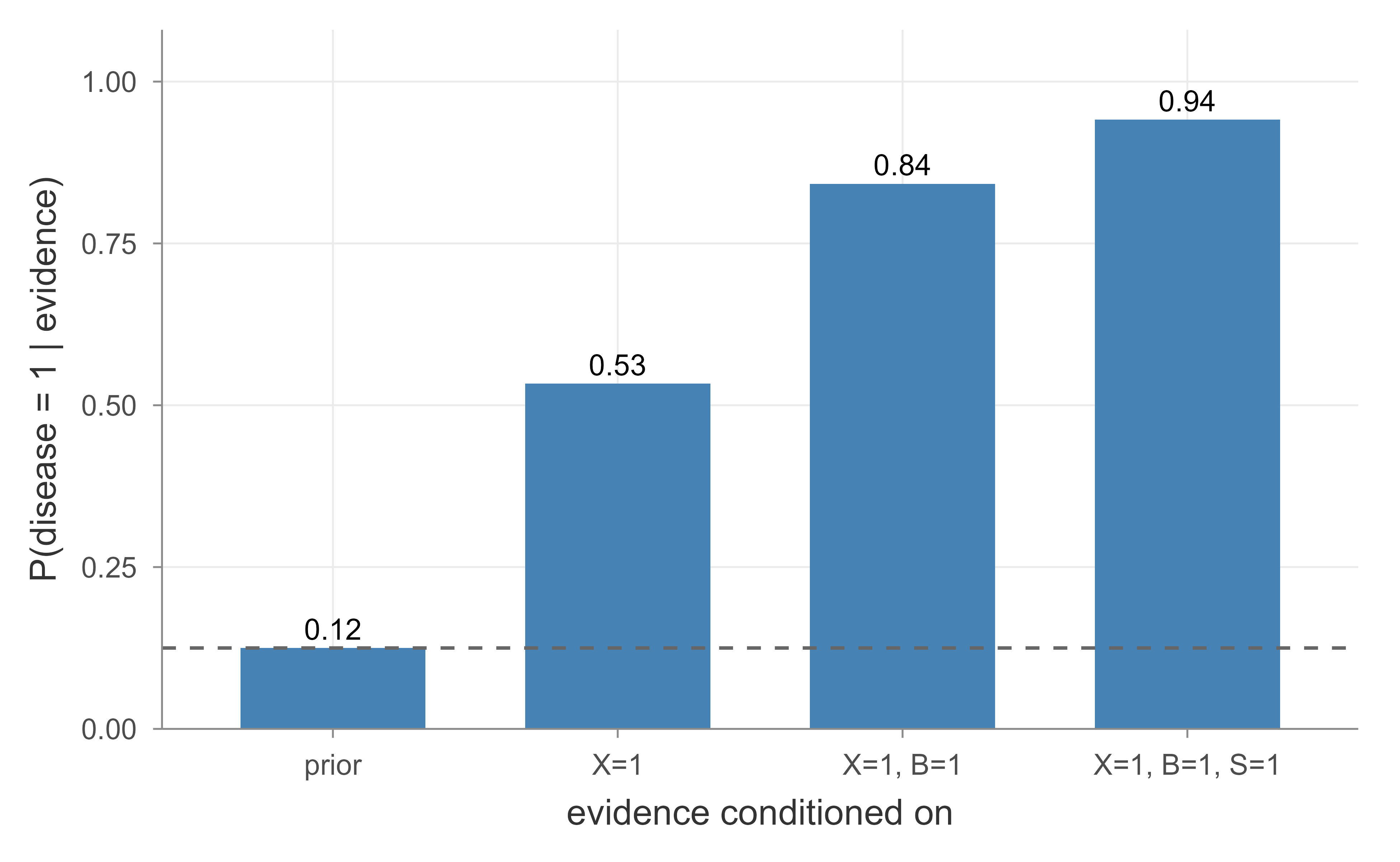
Finally, we visualize how the posterior probability of disease responds to accumulating evidence, the core behavior of a graphical model used for diagnosis.
Figure 73.1: Posterior probability of disease as evidence accumulates. Each bar conditions on more observations, and the dashed line marks the prior base rate, showing how leaf evidence propagates back to the root.
Figure 73.1 shows the posterior climbing steadily as we add a positive X-ray, then breathlessness, then smoking status. The dashed line is the prior, so every bar above it represents evidence raising our belief in disease. This is variable elimination’s payoff seen from the user’s side: structured, interpretable updates to belief as observations arrive.
Scaling up in practice
For real problems do not hand-build the joint. R packages such as gRain and bnlearn represent CPTs, compile a junction tree for efficient exact inference, and learn both parameters and structure from data. The enumeration here is meant to expose the mechanics, not to be used beyond a handful of variables, since it is the very \(O(K^n)\) cost that variable elimination and the junction tree algorithm exist to avoid.
73.7 Connections and Closing Notes
Probabilistic graphical models are a unifying framework rather than a single algorithm, and many methods elsewhere in this book are special cases or close relatives. Naive Bayes (Chapter 18) is the simplest non-trivial Bayes net, a single class node pointing at conditionally independent features. Gaussian graphical models, where zeros in the inverse covariance matrix correspond to missing edges, link the undirected formalism to the multivariate Gaussian reasoning behind Gaussian process regression (Chapter 7) and discriminant analysis (Chapter 20). Hidden Markov models and conditional random fields, the workhorses of sequence labeling in Chapter 77, are graphical models with chain structure, and the max-product algorithm there is the same message passing derived above. When exact inference is intractable, the variational and sampling techniques used for Bayesian deep learning (Chapter 46) and the modeling languages of Chapter 75 take over. The graph is the common thread: it specifies the model, exposes the independences, and dictates the algorithm, so understanding it pays off across the entire probabilistic side of machine learning.
Source Code
# Probabilistic Graphical Models {#sec-graphical-models}```{r}#| include: falsesource("_common.R")```Suppose you want to reason about a small medical scenario. A patient may or may not be a smoker; smoking raises the chance of lung disease; lung disease changes what a chest X-ray shows and whether the patient is short of breath. Written out as one giant table, the joint distribution over (smoker, disease, X-ray, dyspnea) has many cells, and most of them encode relationships that do not actually exist. The X-ray does not depend on whether the patient smokes once we already know whether they have the disease. The X-ray tells us about the disease, the disease tells us about smoking, but the X-ray adds nothing once the disease is fixed.Probabilistic graphical models are a language for writing down exactly which of these relationships are real and which can be dropped. A graph records the dependencies: each variable is a node, and the edges (or their absence) encode conditional independence. The payoff is twofold. First, the joint distribution factorizes into small local pieces, so we store and estimate far fewer numbers. Second, the same graph that compresses the model also tells us how to answer questions about it, such as "given a positive X-ray, how likely is the patient to be a smoker?" This chapter develops both the directed family (Bayesian networks) and the undirected family (Markov random fields), shows how the joint factorizes in each, derives the conditional-independence rules that justify the factorization, works through exact inference by variable elimination, sketches belief propagation, covers parameter learning, and ends with a runnable base-R example that computes a posterior on a four-node Bayes net by brute-force enumeration.::: {.callout-tip title="When to use this"}Reach for a graphical model when you have many interacting variables, you know (or want to learn) the qualitative structure of how they relate, and you need to answer probabilistic queries about some variables given evidence on others. They are the natural home for reasoning under uncertainty with structure, and they connect directly to @sec-naive-bayes (the simplest Bayes net), @sec-discriminant-analysis, and the probabilistic modeling tools in @sec-probabilistic-programming.:::## The Curse of the Full JointEverything we want to know about a set of discrete random variables $X_1, \dots, X_n$ is contained in their joint distribution $p(x_1, \dots, x_n)$. The problem is size. If each $X_i$ takes $K$ values, the joint is a table with $K^n$ entries, and because the entries must sum to one it has $K^n - 1$ free parameters. For $n = 30$ binary variables that is more than a billion numbers, which we can neither store nor estimate from any realistic dataset. The same combinatorial blowup that haunts density estimation in high dimensions (@sec-density-estimation) appears here.The chain rule of probability lets us write the joint exactly, with no assumptions, as a product of conditionals,$$p(x_1, \dots, x_n) = \prod_{i=1}^{n} p(x_i \mid x_1, \dots, x_{i-1}).$$This rewriting does not save anything by itself, because the last factor still conditions on everything before it. The key move of graphical models is to assert that most of those conditioning variables do not matter: each $X_i$ depends only on a small subset of the others. Encoding which subset is exactly what the graph does.::: {.callout-important title="Key idea"}A graphical model is a claim that the joint factorizes into local pieces, each involving only a few variables. The graph is a picture of that factorization, and equivalently a picture of a set of conditional-independence statements. Fewer edges means a stronger claim and fewer parameters.:::## Directed Models: Bayesian NetworksA Bayesian network is a directed acyclic graph (DAG) $G$ with one node per variable, together with one conditional probability distribution (CPD) per node. An edge from $X_j$ to $X_i$ means $X_j$ is a direct cause or parent of $X_i$; write $\mathrm{pa}(i)$ for the set of parents of node $i$. The network asserts that the joint factorizes as a product of each node conditioned on its parents,$$p(x_1, \dots, x_n) = \prod_{i=1}^{n} p\bigl(x_i \mid x_{\mathrm{pa}(i)}\bigr).$$ {#eq-graphical-models-bn-factor}Each factor $p(x_i \mid x_{\mathrm{pa}(i)})$ is a local conditional probability table (CPT) for discrete variables, or a parametric conditional density in the continuous case. The savings are dramatic. A node with $k$ parents, each binary, needs only $2^k$ parameters instead of conditioning on all $n - 1$ predecessors. The medical example factorizes as$$p(s, d, x, b) = p(s)\, p(d \mid s)\, p(x \mid d)\, p(b \mid d),$$with $s$ for smoker, $d$ for disease, $x$ for X-ray, $b$ for breathlessness (dyspnea). Four small tables replace one table of fifteen free parameters.### Why the Factorization Encodes Conditional IndependenceThe factorization in @eq-graphical-models-bn-factor is equivalent to a collection of conditional-independence statements, and it is worth deriving one to see the mechanism. Order the nodes topologically so that every parent precedes its children. Starting from the exact chain rule and substituting the factorization, factor by factor,$$\prod_{i=1}^{n} p(x_i \mid x_1, \dots, x_{i-1}) = \prod_{i=1}^{n} p\bigl(x_i \mid x_{\mathrm{pa}(i)}\bigr),$$which holds for all values if and only if each predecessor set can be replaced by the parent set,$$p(x_i \mid x_1, \dots, x_{i-1}) = p\bigl(x_i \mid x_{\mathrm{pa}(i)}\bigr).$$ {#eq-graphical-models-local-markov}Statement @eq-graphical-models-local-markov is the local Markov property: given its parents, a node is independent of all its other non-descendant predecessors. In the medical net, $p(x \mid s, d) = p(x \mid d)$ says the X-ray is independent of smoking given the disease, exactly the simplification we noticed at the start.### d-Separation: Reading Off Independence from the GraphThe local Markov property gives some independences directly, but the graph implies many more. The tool that reads off every independence the factorization guarantees is **d-separation** (directional separation). Consider a path (ignoring edge direction) between two nodes. The path is *blocked* by a set of observed variables $Z$ according to three local patterns at each intermediate node $w$ on the path:- **Chain** $a \to w \to b$ and **fork** $a \leftarrow w \to b$: the path is blocked if $w \in Z$. Observing the middle variable cuts the flow of information.- **Collider** $a \to w \leftarrow b$ (also called a v-structure): the path is blocked if neither $w$ nor any descendant of $w$ is in $Z$. Here the logic inverts: observing the collider (or its descendant) *opens* the path.Two sets $A$ and $B$ are d-separated by $Z$ if every path between them is blocked. Whenever $A$ and $B$ are d-separated by $Z$, the distribution satisfies $X_A \perp X_B \mid X_Z$.::: {.callout-note}The collider rule is the source of the famous "explaining away" effect. Suppose disease and a separate cause both raise the chance of breathlessness ($d \to b \leftarrow c$). A priori the disease and the other cause are independent. But once we observe breathlessness, learning that the other cause is present lowers the probability of the disease: the two compete to explain the symptom. Conditioning on the collider creates a dependence that was not there before.:::### The Markov BlanketA useful consequence of d-separation is the **Markov blanket** of a node $X_i$, the minimal set that renders $X_i$ independent of everything else. In a Bayesian network the Markov blanket consists of the node's parents, its children, and its children's other parents (co-parents),$$\mathrm{MB}(i) = \mathrm{pa}(i) \cup \mathrm{ch}(i) \cup \Bigl(\bigcup_{j \in \mathrm{ch}(i)} \mathrm{pa}(j) \setminus \{i\}\Bigr).$$Conditioned on its blanket, $X_i \perp X_{\text{rest}} \mid X_{\mathrm{MB}(i)}$. The co-parents appear because of the collider rule: each child is a collider on the path from $X_i$ to that child's other parents, so observing the child opens those paths and they must be included to close them again. The Markov blanket is what local algorithms such as Gibbs sampling and many message-passing schemes need to condition on, so it is the practical unit of computation.## Undirected Models: Markov Random FieldsSometimes there is no natural direction of influence. Neighboring pixels in an image tend to share a label, neighboring sites on a lattice interact, but neither causes the other. For these symmetric situations we use an undirected graph, a **Markov random field** (MRF), also called a Markov network. Here the joint is built not from conditional probabilities but from non-negative **potential functions** $\psi_C$ defined over the cliques $C$ of the graph (a clique is a fully connected subset of nodes). By the Hammersley to Clifford theorem, a strictly positive distribution that satisfies the Markov properties of an undirected graph factorizes over its cliques,$$p(x_1, \dots, x_n) = \frac{1}{Z} \prod_{C \in \mathcal{C}} \psi_C(x_C),\qquadZ = \sum_{x_1, \dots, x_n} \prod_{C \in \mathcal{C}} \psi_C(x_C).$$ {#eq-graphical-models-mrf-factor}The potentials $\psi_C \geq 0$ are arbitrary non-negative functions, not probabilities; they score how compatible a configuration of $x_C$ is. The normalizer $Z$, the **partition function**, sums the unnormalized product over all joint configurations so the distribution integrates to one. Because $Z$ couples every variable together, computing it is the central difficulty of undirected models. It is common to write potentials in exponential form $\psi_C(x_C) = \exp(-E_C(x_C))$, giving the Gibbs (Boltzmann) distribution $p(x) = Z^{-1} \exp(-\sum_C E_C(x_C))$ familiar from statistical physics, where $E$ is the energy and low-energy configurations are most probable.::: {.callout-warning title="The two families are not interchangeable"}Directed and undirected models capture overlapping but different independence sets. A v-structure (collider) cannot be represented by any undirected graph, and an undirected four-cycle cannot be represented by any DAG without adding edges. They also differ operationally: a Bayes net's local factors are already normalized conditionals, so no global $Z$ is needed and ancestral sampling is trivial, whereas an MRF carries an intractable $Z$ in general. Choose the directed form when influence has a natural direction and you want easy sampling; choose the undirected form for symmetric, relational structure such as grids and lattices.:::The Markov properties for an MRF are read directly off the undirected graph: two sets are independent given a third if the third set separates them in the ordinary graph-theoretic sense (every path passes through it). The Markov blanket of a node in an MRF is simply its set of graph neighbors, which is much simpler than the directed case because there are no colliders to worry about.## Exact Inference by Variable EliminationGiven a model, the queries we care about are marginals such as $p(x_q)$ and conditionals such as $p(x_q \mid x_E = e)$ for a query node $q$ and evidence $E$. The naive approach sums the full joint over the non-query, non-evidence variables, which costs $O(K^n)$ and defeats the purpose of the factorization. **Variable elimination** exploits the factorized form to push sums inside products and reuse work.The idea is the distributive law. To marginalize out a variable, we gather only the factors that mention it, sum over it once, and replace them with the resulting smaller factor. Consider a chain $A \to B \to C \to D$ with joint $p(a)p(b\mid a)p(c\mid b)p(d\mid c)$, and suppose we want $p(d)$. Eliminating $a, b, c$ in turn,$$p(d) = \sum_{c} p(d \mid c) \sum_{b} p(c \mid b) \sum_{a} p(b \mid a)\, p(a).$$ {#eq-graphical-models-ve}The innermost sum $\sum_a p(b\mid a)p(a)$ produces a factor over $b$ alone, call it $m_1(b)$; the next sum $\sum_b p(c\mid b) m_1(b)$ produces $m_2(c)$; the last produces $p(d)$. Each step sums over one variable inside a factor whose size is bounded by the number of variables it touches, not by $n$. For the chain, each intermediate factor involves at most two variables, so the cost is $O(n K^2)$ rather than $O(K^n)$: an exponential saving turned linear.::: {.callout-note title="Intermediate factors are not probabilities"}The functions $m_1, m_2, \dots$ produced during elimination are sometimes called messages. They need not sum to one; they are just partial sums of the joint. Only the final result, after restoring evidence and normalizing, is a probability. This is the same bookkeeping that lets us drop the denominator in Bayes' rule and restore it at the end.:::To answer a conditional query $p(x_q \mid x_E = e)$ we first fix the evidence variables to their observed values (which simply selects slices of the relevant factors), run elimination on the remaining non-query variables to obtain the unnormalized $\tilde p(x_q, e)$, and then normalize over $x_q$,$$p(x_q \mid x_E = e) = \frac{\tilde p(x_q, e)}{\sum_{x_q} \tilde p(x_q, e)}.$$### Complexity and the Elimination OrderThe cost of variable elimination is dominated by the largest intermediate factor created, whose size is $K$ raised to the number of variables it touches. That number, minus one, taken over the best possible elimination order, is the **treewidth** of the graph. For trees the treewidth is one and inference is linear; for dense graphs it can be $O(n)$, and then exact inference is exponential and intractable. Finding the optimal elimination order is itself NP-hard, so in practice we use greedy heuristics such as min-fill or min-degree. The lesson is that exact inference is efficient exactly when the graph is sparse and tree-like, and is hopeless for densely connected models, where we fall back on approximate methods.### Belief PropagationOn a tree, variable elimination has an elegant reformulation as **belief propagation** (the sum-product algorithm), which computes all marginals at once rather than one query at a time. Each node sends a message to each neighbor summarizing everything it knows from the rest of the graph. The message from node $j$ to node $i$ collects $j$'s local factor and the incoming messages from $j$'s other neighbors $\mathcal{N}(j) \setminus \{i\}$, then sums out $j$,$$m_{j \to i}(x_i) = \sum_{x_j} \psi_j(x_j)\, \psi_{ij}(x_i, x_j) \prod_{k \in \mathcal{N}(j) \setminus \{i\}} m_{k \to j}(x_j).$$ {#eq-graphical-models-bp}Once messages have flowed in both directions across every edge (two passes on a tree, leaves inward then root outward), the marginal at any node is the product of its local factor and all incoming messages, normalized,$$p(x_i) \propto \psi_i(x_i) \prod_{k \in \mathcal{N}(i)} m_{k \to i}(x_i).$$On a tree this is exact and costs $O(n K^2)$. On a graph with cycles the same update rule can be iterated, giving **loopy belief propagation**, which is no longer guaranteed to be exact or even to converge, yet is often an excellent approximation and underlies decoding in modern error-correcting codes. Replacing the sum in @eq-graphical-models-bp with a max gives the max-product algorithm, the analogue that finds the most probable joint configuration, closely related to the structured-prediction inference of @sec-structured-prediction.## Learning the ParametersSo far the CPDs or potentials were given. With a fully observed discrete dataset $\{x^{(1)}, \dots, x^{(m)}\}$ and a fixed DAG, learning a Bayesian network's parameters by maximum likelihood is remarkably clean because the log-likelihood decomposes over nodes. Writing the likelihood and taking the log,$$\log p(\text{data}) = \sum_{t=1}^{m} \sum_{i=1}^{n} \log p\bigl(x_i^{(t)} \mid x_{\mathrm{pa}(i)}^{(t)}\bigr)= \sum_{i=1}^{n} \sum_{t=1}^{m} \log p\bigl(x_i^{(t)} \mid x_{\mathrm{pa}(i)}^{(t)}\bigr).$$ {#eq-graphical-models-loglik}The double sum separates into independent per-node problems, and each one further separates by the parent configuration. The maximum-likelihood estimate of each CPT entry is just an empirical conditional frequency, the count of co-occurrences divided by the count of the parent configuration,$$\hat p\bigl(x_i = v \mid x_{\mathrm{pa}(i)} = u\bigr) = \frac{N(x_i = v,\; x_{\mathrm{pa}(i)} = u)}{N(x_{\mathrm{pa}(i)} = u)},$$ {#eq-graphical-models-mle}where $N(\cdot)$ counts matching rows. To avoid zero estimates from unseen configurations one adds pseudo-counts (a Dirichlet prior), giving the Bayesian estimate with Laplace-style smoothing, exactly the device used in @sec-naive-bayes.::: {.callout-important title="Two hard cases"}Closed-form counting works only when (1) the structure is known and (2) all variables are observed. With hidden variables the log-likelihood no longer decomposes and we use Expectation to Maximization, alternating between inferring the missing values (an inference query) and re-estimating parameters. Learning the structure itself (which edges to include) is a search over DAGs scored by penalized likelihood (BIC) or marginal likelihood, and is NP-hard in general. Undirected models are harder still: the gradient of the log-likelihood involves expectations under the model that require the intractable $Z$, so one resorts to approximate gradients (contrastive divergence) or pseudo-likelihood.:::## A Worked Example in Base RWe now build the four-node medical Bayes net, $S \to D$, $D \to X$, $D \to B$, and compute a posterior by brute-force enumeration of the joint. Enumeration is the naive baseline that variable elimination improves on; for four binary nodes the full joint has only $16$ rows, so it is fast and lets us check our reasoning exactly. We use only base R.```{r}#| label: graphical-models-bayesnet# Four-node Bayes net: S (smoker) -> D (disease) -> {X (x-ray), B (dyspnea)}# All variables binary, coded 0 = no/absent, 1 = yes/present.# --- Conditional probability tables (the local factors) ----------------------p_S <-c("0"=0.7, "1"=0.3) # P(S)# P(D | S): rows indexed by S, columns give P(D = 0), P(D = 1)p_D_given_S <-rbind("S=0"=c(0.95, 0.05),"S=1"=c(0.70, 0.30))# P(X | D): rows indexed by Dp_X_given_D <-rbind("D=0"=c(0.90, 0.10),"D=1"=c(0.20, 0.80))# P(B | D): rows indexed by Dp_B_given_D <-rbind("D=0"=c(0.85, 0.15),"D=1"=c(0.30, 0.70))# --- Build the full joint by enumerating all 2^4 = 16 configurations ----------grid <-expand.grid(S =0:1, D =0:1, X =0:1, B =0:1)grid$p <-with(grid, p_S[S +1] * p_D_given_S[cbind(S +1, D +1)] * p_X_given_D[cbind(D +1, X +1)] * p_B_given_D[cbind(D +1, B +1)])cat("Sum of joint (should be 1):", round(sum(grid$p), 12), "\n")```The joint sums to one, confirming the factorization and the CPTs are consistent. Now we answer queries by summing the relevant rows of `grid`, which is exactly enumeration-based inference.```{r}#| label: graphical-models-queries# Helper: probability of a logical condition under the jointprob <-function(cond) sum(grid$p[cond])# Prior marginal P(D = 1): disease before any evidencep_disease <-prob(grid$D ==1)# Posterior P(S = 1 | X = 1): is the patient a smoker, given a positive x-ray?# P(S=1, X=1) / P(X=1)post_smoker <-prob(grid$S ==1& grid$X ==1) /prob(grid$X ==1)# Posterior P(D = 1 | X = 1, B = 1): disease given positive x-ray AND dyspneapost_disease <-prob(grid$D ==1& grid$X ==1& grid$B ==1) /prob(grid$X ==1& grid$B ==1)results <-data.frame(query =c("P(D=1) prior","P(S=1 | X=1)","P(D=1 | X=1, B=1)"),probability =round(c(p_disease, post_smoker, post_disease), 4))print(results, row.names =FALSE)```The prior disease rate is low, but conditioning on a positive X-ray raises the posterior probability that the patient is a smoker well above the base rate of $0.3$, and conditioning on both a positive X-ray and breathlessness pushes the disease posterior sharply upward. Evidence at the leaves flows back up the network to the root, which is the whole point of probabilistic inference.We can also verify the conditional independence that d-separation promises: the X-ray and smoking should be independent once the disease is known, $p(X \mid D, S) = p(X \mid D)$.```{r}#| label: graphical-models-dsep# Check X _|_ S | D by comparing P(X=1 | D=1, S=0) and P(X=1 | D=1, S=1)pXgivenDS0 <-prob(grid$X ==1& grid$D ==1& grid$S ==0) /prob(grid$D ==1& grid$S ==0)pXgivenDS1 <-prob(grid$X ==1& grid$D ==1& grid$S ==1) /prob(grid$D ==1& grid$S ==1)cat("P(X=1 | D=1, S=0) =", round(pXgivenDS0, 6), "\n")cat("P(X=1 | D=1, S=1) =", round(pXgivenDS1, 6), "\n")cat("Equal (X _|_ S | D)?", isTRUE(all.equal(pXgivenDS0, pXgivenDS1)), "\n")```The two conditional probabilities are identical, confirming that smoking carries no extra information about the X-ray once the disease is known, exactly as the graph structure $S \to D \to X$ predicts via d-separation.Finally, we visualize how the posterior probability of disease responds to accumulating evidence, the core behavior of a graphical model used for diagnosis.```{r}#| label: fig-graphical-models-posterior#| fig-cap: "Posterior probability of disease as evidence accumulates. Each bar conditions on more observations, and the dashed line marks the prior base rate, showing how leaf evidence propagates back to the root."ev_labels <-c("prior", "X=1", "X=1, B=1", "X=1, B=1, S=1")ev_probs <-c(prob(grid$D ==1),prob(grid$D ==1& grid$X ==1) /prob(grid$X ==1),prob(grid$D ==1& grid$X ==1& grid$B ==1) /prob(grid$X ==1& grid$B ==1),prob(grid$D ==1& grid$X ==1& grid$B ==1& grid$S ==1) /prob(grid$X ==1& grid$B ==1& grid$S ==1))df <-data.frame(evidence =factor(ev_labels, levels = ev_labels),posterior = ev_probs)ggplot(df, aes(x = evidence, y = posterior)) +geom_col(fill ="steelblue", width =0.65) +geom_hline(yintercept = ev_probs[1], linetype ="dashed", colour ="grey40") +geom_text(aes(label =sprintf("%.2f", posterior)), vjust =-0.4, size =3.5) +scale_y_continuous(limits =c(0, 1), expand =expansion(mult =c(0, 0.08))) +labs(x ="evidence conditioned on", y ="P(disease = 1 | evidence)") +theme_book()```@fig-graphical-models-posterior shows the posterior climbing steadily as we add a positive X-ray, then breathlessness, then smoking status. The dashed line is the prior, so every bar above it represents evidence raising our belief in disease. This is variable elimination's payoff seen from the user's side: structured, interpretable updates to belief as observations arrive.::: {.callout-tip title="Scaling up in practice"}For real problems do not hand-build the joint. R packages such as `gRain` and `bnlearn` represent CPTs, compile a junction tree for efficient exact inference, and learn both parameters and structure from data. The enumeration here is meant to expose the mechanics, not to be used beyond a handful of variables, since it is the very $O(K^n)$ cost that variable elimination and the junction tree algorithm exist to avoid.:::## Connections and Closing NotesProbabilistic graphical models are a unifying framework rather than a single algorithm, and many methods elsewhere in this book are special cases or close relatives. Naive Bayes (@sec-naive-bayes) is the simplest non-trivial Bayes net, a single class node pointing at conditionally independent features. Gaussian graphical models, where zeros in the inverse covariance matrix correspond to missing edges, link the undirected formalism to the multivariate Gaussian reasoning behind Gaussian process regression (@sec-gaussian-process-reg) and discriminant analysis (@sec-discriminant-analysis). Hidden Markov models and conditional random fields, the workhorses of sequence labeling in @sec-structured-prediction, are graphical models with chain structure, and the max-product algorithm there is the same message passing derived above. When exact inference is intractable, the variational and sampling techniques used for Bayesian deep learning (@sec-bayesian-deep-learning) and the modeling languages of @sec-probabilistic-programming take over. The graph is the common thread: it specifies the model, exposes the independences, and dictates the algorithm, so understanding it pays off across the entire probabilistic side of machine learning.