Suppose you measure a single number on a large group of people, say their annual income, and plot a histogram. Instead of one tidy bell curve you see two humps: a tall one over modest salaries and a shorter, wider one stretching off to the right. No single Gaussian can describe that picture, yet it would be a shame to abandon the convenience of Gaussians altogether. The natural fix is to imagine that the population is really a blend of two subpopulations, each roughly Gaussian on its own, and that what we see is their mixture. We do not know who belongs to which group, and we do not know the groups’ means, spreads, or relative sizes. Recovering all of that from the unlabeled numbers alone is the problem this chapter solves.
A Gaussian mixture model (GMM) makes that intuition precise. It says the data come from \(K\) Gaussian components, and every observation was generated by first secretly drawing a component and then drawing a point from that component’s Gaussian. The “secret” label is a latent variable: present in the generative story, absent from the data. The expectation-maximization (EM) algorithm is the engine that fits such latent-variable models, alternating between guessing the hidden labels and re-estimating the parameters those labels imply.
This chapter sits at the meeting point of two earlier ones. As a clustering method, the GMM is the probabilistic cousin of k-means from the cluster analysis chapter (Chapter 23): instead of assigning each point hard to one group, it gives a soft, probabilistic membership, and we will see that k-means is exactly the limiting case where the soft assignments harden. As a density model, the GMM is the parametric workhorse introduced in the density estimation chapter (Chapter 32), capable of approximating almost any smooth density given enough components. EM itself reaches well beyond mixtures: it is the standard tool for hidden Markov models, factor analysis, and the missing-data problems that show up throughout statistics.
Note
The density estimation chapter (Chapter 32) presents the GMM briefly as one tool for estimating \(p(x)\). This chapter is the full treatment: the latent-variable construction, the complete EM derivation with its monotonicity guarantee, the link to k-means, covariance parameterizations, model selection by BIC, and a from-scratch implementation you can run.
24.1 The model
We observe \(x_1, \ldots, x_n\) with each \(x_i \in \mathbb{R}^d\), assumed independent. A Gaussian mixture with \(K\) components models the density of a single observation as a weighted sum of Gaussians,
where \(\mathcal{N}(x \mid \mu_k, \Sigma_k)\) is the multivariate normal density with mean \(\mu_k\) and covariance \(\Sigma_k\), and the mixing weights\(\pi_k\) are nonnegative and sum to one,
The full parameter vector is \(\theta = \{\pi_k, \mu_k, \Sigma_k\}_{k=1}^{K}\). Equation Equation 24.1 is a perfectly good density (a convex combination of densities is a density), but on its own it hides what makes the model tractable. The key is to read it as the marginal of a richer generative process.
24.1.1 The latent-variable view
Introduce for each observation a hidden label \(z_i \in \{1, \ldots, K\}\) saying which component produced it. It is convenient to write \(z_i\) as a one-hot vector \((z_{i1}, \ldots, z_{iK})\) with \(z_{ik} = 1\) if observation \(i\) came from component \(k\) and zero otherwise. The generative story is two steps:
First draw a component with probability \(\pi_k\), then draw the point from that component’s Gaussian. Marginalizing the latent label recovers Equation 24.1, because
So the mixture is what you get when you forget the labels. This is the same trick used throughout latent-variable modeling, and it is why mixtures connect naturally to the probabilistic models in Chapter 42, where the latent variable is continuous rather than discrete.
24.1.2 Responsibilities
Once we have parameters, we can ask the reverse question: given that we observed \(x_i\), what is the posterior probability that component \(k\) produced it? By Bayes’ rule,
The quantity \(\gamma_{ik}\) is called the responsibility that component \(k\) takes for observation \(i\). By construction \(\sum_k \gamma_{ik} = 1\), so each point’s unit of “membership” is split softly across components in proportion to how well each component explains it, weighted by how prevalent that component is. These responsibilities are the soft assignments that distinguish a GMM from k-means, and they are the central object EM computes.
24.1.3 The likelihood we want to maximize
Fitting the model by maximum likelihood means choosing \(\theta\) to maximize the log-likelihood of the observed data,
The trouble is the logarithm of a sum. We cannot push the \(\log\) inside the \(\sum_k\), so the score equations couple all components together and have no closed-form solution. If we knew the labels \(z_i\), the picture would be trivial: the complete-data log-likelihood would be a sum of separate Gaussian fits,
whose \(\log\) now sits on a single Gaussian and maximizes in closed form. EM exploits exactly this gap: it replaces the unknown \(z_{ik}\) with their expected values (the responsibilities) and then maximizes as if the labels were known.
24.2 Deriving the EM algorithm
We give two derivations. The first is the direct route: take the derivatives of Equation 24.5 and read off a fixed-point iteration. The second, the evidence-lower-bound view, explains why that iteration is guaranteed to improve the likelihood every step.
24.2.1 M-step updates by direct differentiation
Hold the responsibilities fixed at their current values and differentiate the log-likelihood. Recall that for a Gaussian, \(\log \mathcal{N}(x \mid \mu_k, \Sigma_k) = -\tfrac12 \log|2\pi\Sigma_k| - \tfrac12 (x-\mu_k)^\top \Sigma_k^{-1}(x-\mu_k)\). Differentiating Equation 24.5 with respect to \(\mu_k\) and using \(\partial \ell / \partial \mu_k = \sum_i \gamma_{ik}\, \Sigma_k^{-1}(x_i - \mu_k)\) (the responsibility appears because it is exactly the derivative of the outer \(\log\) times the prior weight), setting the gradient to zero gives the weighted mean
Here \(N_k\) is the effective number of points assigned to component \(k\), the soft analogue of a cluster size. Differentiating with respect to \(\Sigma_k\) (treating it as a symmetric positive-definite matrix) and zeroing the gradient yields the responsibility-weighted covariance
For the weights we must respect the constraint Equation 24.2. Maximize \(\sum_i \log p(x_i) + \lambda\bigl(\sum_k \pi_k - 1\bigr)\) over \(\pi_k\) with a Lagrange multiplier \(\lambda\). The stationarity condition is \(\sum_i \gamma_{ik}/\pi_k + \lambda = 0\), so \(\pi_k = -N_k/\lambda\); summing over \(k\) and using \(\sum_k \pi_k = 1\) fixes \(\lambda = -n\), giving
\[
\pi_k \;=\; \frac{N_k}{n}.
\tag{24.9}\]
These three updates are the M-step. Each is a familiar Gaussian estimator with the hard count replaced by the soft responsibility weight. The catch is that all three depend on \(\gamma_{ik}\), which in turn depends on the parameters through Equation 24.4. That circularity is what makes this a fixed-point iteration rather than a closed-form solution, and it defines the algorithm.
The algorithm in one breath
Initialize \(\theta\). Then iterate until convergence: E-step, compute responsibilities \(\gamma_{ik}\) from Equation 24.4 using the current \(\theta\); M-step, update \(\pi_k, \mu_k, \Sigma_k\) from Equation 24.9, Equation 24.7, Equation 24.8 using those responsibilities. Each full pass cannot decrease Equation 24.5.
24.2.2 The evidence lower bound and why likelihood never decreases
The direct derivation gives the updates but not the guarantee. For that we introduce, for each observation, an arbitrary distribution \(q_i(z)\) over the latent label and apply Jensen’s inequality to the log-likelihood. For any \(q_i\) with \(q_i(k) > 0\),
since KL divergence is nonnegative and zero only when its two arguments coincide. EM is now visibly coordinate ascent on \(\mathcal{L}(q,\theta)\):
E-step (maximize over \(q\), \(\theta\) fixed). The bound Equation 24.12 is tightest, in fact equal to \(\ell(\theta)\), when each \(q_i\) equals the posterior \(p(z \mid x_i, \theta)\), which is precisely the responsibility \(\gamma_{ik}\) of Equation 24.4. After the E-step the bound touches the likelihood: \(\mathcal{L}(\gamma, \theta) = \ell(\theta)\).
M-step (maximize over \(\theta\), \(q = \gamma\) fixed). Dropping the \(\theta\)-free entropy term \(-\sum_{i,k}\gamma_{ik}\log\gamma_{ik}\), maximizing \(\mathcal{L}\) over \(\theta\) means maximizing the expected complete-data log-likelihood \(\sum_{i,k}\gamma_{ik}[\log\pi_k + \log\mathcal{N}(x_i\mid\mu_k,\Sigma_k)]\), whose solution is exactly the M-step updates Equation 24.9, Equation 24.7, Equation 24.8.
The monotonicity argument is now a two-line chain. Let \(\theta^{(t)}\) be the current parameters and \(\theta^{(t+1)}\) the result of one E-then-M cycle. The E-step makes the bound tight, \(\mathcal{L}(\gamma^{(t)}, \theta^{(t)}) = \ell(\theta^{(t)})\); the M-step can only raise the bound, \(\mathcal{L}(\gamma^{(t)}, \theta^{(t+1)}) \ge \mathcal{L}(\gamma^{(t)}, \theta^{(t)})\); and the bound always sits below the likelihood, \(\ell(\theta^{(t+1)}) \ge \mathcal{L}(\gamma^{(t)}, \theta^{(t+1)})\). Chaining these,
So the observed-data log-likelihood is nondecreasing at every iteration. Since a correctly regularized GMM likelihood is bounded above, the sequence \(\ell(\theta^{(t)})\) converges. This is the property we will check numerically: the log-likelihood curve must rise monotonically.
Convergence is to a local optimum, not the global one
Monotone ascent guarantees the likelihood climbs, but not that it climbs to the best possible value. The likelihood surface Equation 24.5 is non-convex and riddled with local maxima (and, as Section 24.6 explains, with singularities where it diverges to \(+\infty\)). Different initializations generally land at different local optima. The standard remedy is several random restarts, keeping the run with the highest final likelihood.
24.3 Relation to k-means
K-means from Chapter 23 is not a separate idea bolted on; it is the GMM in a specific limit. Take all components to share a common spherical, fixed covariance \(\Sigma_k = \sigma^2 I\) and equal weights \(\pi_k = 1/K\), then let \(\sigma^2 \to 0\). The responsibility Equation 24.4 becomes
As \(\sigma^2 \to 0\) this softmax sharpens into an indicator: all the mass collapses onto the single nearest center, \(\gamma_{ik} \to 1\) for \(k = \arg\min_j \|x_i - \mu_j\|^2\) and \(0\) otherwise. The soft E-step becomes the hard nearest-center assignment of k-means, and the M-step mean update Equation 24.7 reduces to the ordinary cluster average. In this light:
K-means is hard EM for an isotropic, equal-weight Gaussian mixture with vanishing variance.
The GMM generalizes k-means in three ways it cannot do: clusters of different sizes (via \(\pi_k\)), different spreads and shapes (via \(\Sigma_k\)), and soft membership that quantifies uncertainty for points sitting between clusters.
This explains a well-known failure of k-means, that it carves space into straight-edged Voronoi cells and so cannot represent elongated or overlapping clusters. A full-covariance GMM, having ellipsoidal contours, handles exactly those cases. The price is more parameters to estimate and more ways to overfit.
24.4 Covariance parameterizations
The covariance \(\Sigma_k\) is where most of the modeling choice lives, because it controls each component’s shape and how many parameters the model spends. A full \(d \times d\) covariance has \(d(d+1)/2\) free entries per component, which grows quadratically in dimension and quickly outpaces the data. Restricting the covariance trades flexibility for stability. The common families, in order of increasing freedom, are summarized in Table 24.1.
Table 24.1: Covariance parameterizations for a Gaussian mixture, from most restrictive to most flexible. Fewer parameters means more stable estimation but less ability to capture cluster shape.
The M-step changes only slightly across these families. For a diagonal model, keep only the diagonal of Equation 24.8. For a spherical model, average that diagonal into a single scalar. For a tied model, pool the per-component scatter into one shared matrix, \(\Sigma = \tfrac1n \sum_{i,k} \gamma_{ik}(x_i-\mu_k)(x_i-\mu_k)^\top\). The popular mclust package indexes a fuller catalogue by a three-letter code (volume, shape, orientation each free or fixed), but the four rows above capture the essential dial. A sensible default workflow is to start diagonal or tied, and only move to full covariances if the data clearly show correlated, differently oriented clusters and you have enough observations per component to estimate \(d(d+1)/2\) numbers reliably.
24.5 Choosing the number of components
The likelihood Equation 24.5 always increases as you add components, so it cannot tell you how many to use; more components fit the training data better by construction. We need a criterion that penalizes complexity. The Bayesian information criterion (BIC) does this. For a model with \(\theta\) fit by maximum likelihood,
\[
\mathrm{BIC} \;=\; -2\,\ell(\hat\theta) + m \log n,
\tag{24.15}\]
where \(m\) is the number of free parameters and \(n\) the sample size. Lower BIC is better. The first term rewards fit, the second penalizes each parameter by \(\log n\), a steeper penalty than AIC’s factor of \(2\), so BIC tends to choose more parsimonious models. The parameter count for a \(K\)-component full-covariance GMM in \(d\) dimensions is
\[
m \;=\; \underbrace{(K-1)}_{\text{weights}} \;+\; \underbrace{Kd}_{\text{means}}
\;+\; \underbrace{K\,\tfrac{d(d+1)}{2}}_{\text{covariances}},
\tag{24.16}\]
with the \(-1\) on the weights because they sum to one. The practical recipe is to fit the model for a range of \(K\) (and, if you like, several covariance families), compute Equation 24.15 for each, and pick the combination minimizing BIC. Because EM only finds local optima, each \((K, \text{family})\) should itself be fit from several random starts before its BIC is recorded.
Note
BIC has an asymptotic Bayesian justification: \(-\tfrac12 \mathrm{BIC}\) approximates the log marginal likelihood (the log evidence) of the model. That is why it is the conventional default for mixtures. It is still an approximation, and for clustering you may legitimately prefer a slightly richer model than BIC’s minimum if the extra component is interpretable. Treat the criterion as a guide, not a verdict.
24.6 Failure modes and practical notes
EM for GMMs is reliable but has sharp edges worth naming.
Covariance singularities. If one component latches onto a single point and shrinks its variance toward zero, that point’s density in Equation 24.5 diverges and the likelihood runs off to \(+\infty\). The global maximum of an unregularized GMM likelihood is therefore infinite and meaningless. The fix is to add a small ridge \(\varepsilon I\) to each \(\Sigma_k\) in the M-step (a form of regularization), or equivalently to put a weak prior on the covariances and maximize the posterior instead.
Label switching. The likelihood is invariant to permuting the component labels, so the “component 1” of two runs need not refer to the same cluster. This is harmless for density estimation but matters if you interpret individual components.
Initialization sensitivity. Because the surface is non-convex, results depend on the start. Initializing means with a k-means run (itself restarted a few times) is the standard, effective default. Always use multiple restarts and keep the best.
Slow convergence near ridges. EM can crawl when components overlap heavily. It still converges, but the last digits of the log-likelihood may take many iterations; stop on a relative-change threshold rather than waiting for exact equality.
Cost. Each iteration is \(O(nKd^2)\) for the responsibilities and weighted scatter, plus \(O(Kd^3)\) for inverting and taking determinants of the covariances. This is cheap in low dimensions and the reason GMMs are a moderate-dimension tool; for very high \(d\) you restrict the covariance or reduce dimension first (Chapter 27).
24.7 A from-scratch EM implementation
We now fit a two-component GMM in base R, with no clustering packages, and verify the central theoretical claim: the log-likelihood increases every iteration. We simulate from a known two-component 1-D mixture, run our own E-step and M-step, and track the log-likelihood.
Show code
set.seed(1301)## --- simulate a 2-component 1-D mixture --------------------------------n<-600pi_true<-c(0.35, 0.65)mu_true<-c(-2.0, 2.5)sd_true<-c(0.8, 1.3)z<-sample(1:2, n, replace =TRUE, prob =pi_true)x<-rnorm(n, mean =mu_true[z], sd =sd_true[z])## --- helper: normal density (base R) -----------------------------------gauss<-function(x, mu, sigma)dnorm(x, mean =mu, sd =sigma)## --- EM for a K-component 1-D Gaussian mixture --------------------------em_gmm<-function(x, K=2, max_iter=200, tol=1e-8, ridge=1e-6){n<-length(x)## initialize: spread means over quantiles, equal weights, marginal sdmu<-as.numeric(quantile(x, probs =(seq_len(K)-0.5)/K))sigma<-rep(sd(x), K)pi_k<-rep(1/K, K)loglik<-numeric(0)for(itinseq_len(max_iter)){## E-step: responsibilities (n x K)dens<-sapply(seq_len(K), function(k)pi_k[k]*gauss(x, mu[k], sigma[k]))mix<-rowSums(dens)gamma<-dens/mix## observed-data log-likelihood with current parametersll<-sum(log(mix))loglik<-c(loglik, ll)## M-stepNk<-colSums(gamma)pi_k<-Nk/nmu<-colSums(gamma*x)/Nkvar_k<-sapply(seq_len(K), function(k)sum(gamma[, k]*(x-mu[k])^2)/Nk[k])sigma<-sqrt(var_k+ridge)# ridge guards against collapse## stop on relative change in log-likelihoodif(it>1&&abs(loglik[it]-loglik[it-1])<tol*abs(loglik[it-1]))break}list(pi =pi_k, mu =mu, sigma =sigma, gamma =gamma, loglik =loglik)}fit<-em_gmm(x, K =2)## --- verify monotonic increase of the log-likelihood -------------------diffs<-diff(fit$loglik)cat("Iterations run: ", length(fit$loglik), "\n")#> Iterations run: 27cat("Min step in log-lik: ", format(min(diffs), digits =4), "\n")#> Min step in log-lik: 6.224e-06cat("Monotonically increasing:", all(diffs>=-1e-9), "\n\n")#> Monotonically increasing: TRUE## --- compare recovered vs. true parameters (sorted by mean) ------------ord<-order(fit$mu)est<-data.frame( component =1:2, pi_hat =round(fit$pi[ord], 3), pi_true =pi_true, mu_hat =round(fit$mu[ord], 3), mu_true =mu_true, sd_hat =round(fit$sigma[ord], 3), sd_true =sd_true)print(est, row.names =FALSE)#> component pi_hat pi_true mu_hat mu_true sd_hat sd_true#> 1 0.313 0.35 -1.984 -2.0 0.787 0.8#> 2 0.687 0.65 2.457 2.5 1.296 1.3
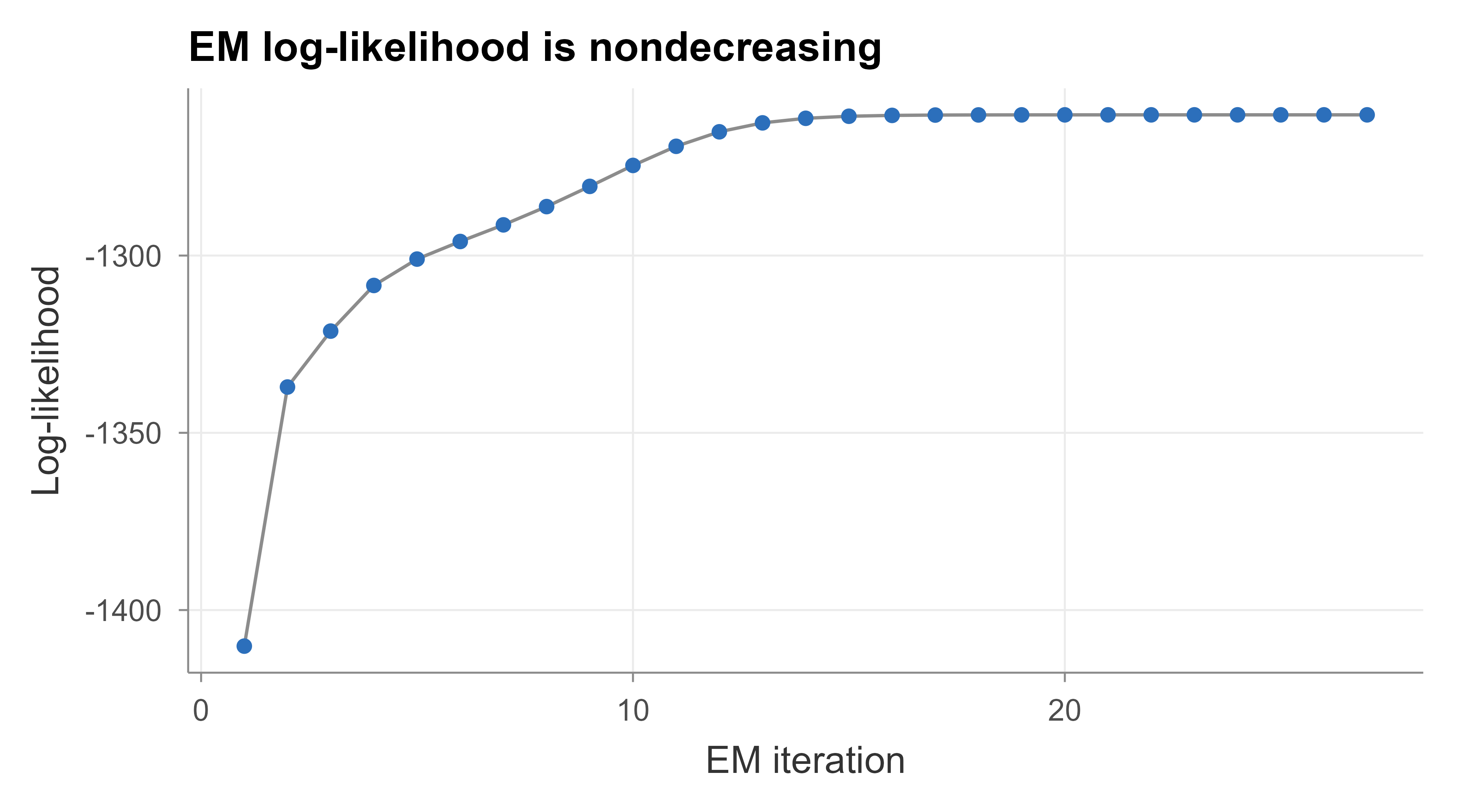
The printed check confirms Monotonically increasing: TRUE: every EM step raised the observed-data log-likelihood, exactly as Equation 24.13 promised, and the smallest step is nonnegative. The recovered weights, means, and standard deviations sit close to the values we simulated from.
Figure 24.1 shows the log-likelihood climbing and leveling off, the visual signature of monotone convergence to a local optimum.
Show code
ll_df<-data.frame(iter =seq_along(fit$loglik), loglik =fit$loglik)ggplot(ll_df, aes(iter, loglik))+geom_line(colour ="grey55", linewidth =0.5)+geom_point(colour ="#2c6fbb", size =1.6)+labs(x ="EM iteration", y ="Log-likelihood", title ="EM log-likelihood is nondecreasing")+theme_book()
Figure 24.1: Observed-data log-likelihood at each EM iteration. It increases monotonically and flattens as the algorithm converges, matching the guarantee derived from the evidence lower bound.
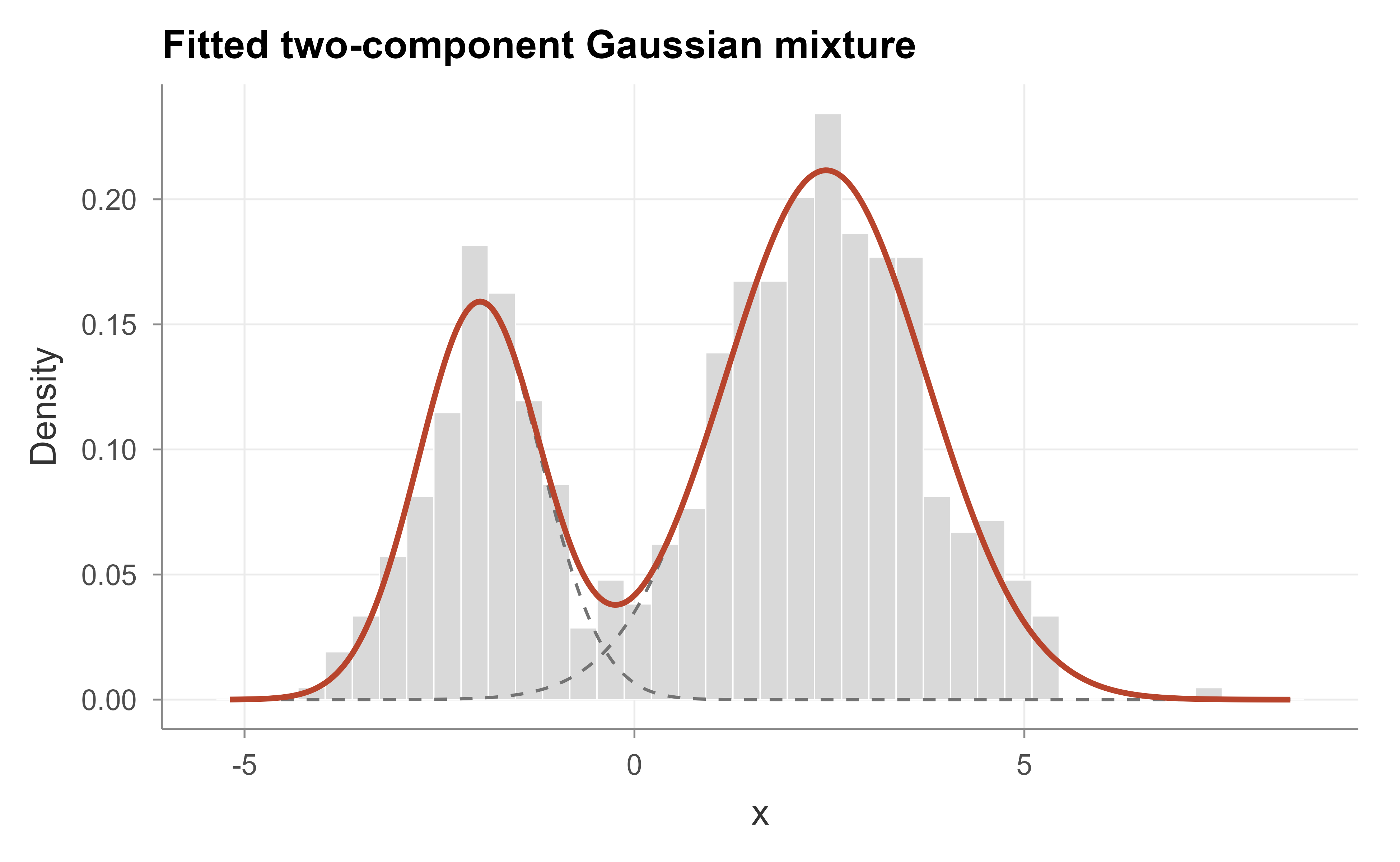
Finally Figure 24.2 overlays the fitted two-component mixture density on a histogram of the data. The estimated mixture (solid) tracks the bimodal shape, and the two dashed curves show the individual weighted components \(\pi_k \mathcal{N}(x \mid \mu_k, \sigma_k)\) that add up to it.
Show code
grid<-seq(min(x)-1, max(x)+1, length.out =400)comp1<-fit$pi[1]*dnorm(grid, fit$mu[1], fit$sigma[1])comp2<-fit$pi[2]*dnorm(grid, fit$mu[2], fit$sigma[2])dens_df<-data.frame( grid =rep(grid, 3), density =c(comp1+comp2, comp1, comp2), curve =rep(c("Mixture", "Component", "Component"), each =length(grid)), piece =rep(c("mix", "c1", "c2"), each =length(grid)))ggplot()+geom_histogram(data =data.frame(x =x), aes(x, after_stat(density)), bins =40, fill ="grey85", colour ="white", linewidth =0.2)+geom_line(data =subset(dens_df, curve=="Component"),aes(grid, density, group =piece), linetype ="dashed", colour ="grey45", linewidth =0.5)+geom_line(data =subset(dens_df, curve=="Mixture"),aes(grid, density), colour ="#b8442c", linewidth =0.9)+labs(x ="x", y ="Density", title ="Fitted two-component Gaussian mixture")+theme_book()
Figure 24.2: Histogram of the simulated data with the fitted GMM density (solid) and its two weighted components (dashed). The mixture captures the bimodal structure a single Gaussian could not.
24.7.1 Selecting K by BIC
To close the loop on model selection, we fit the mixture for \(K = 1, \ldots, 5\) and compute BIC from Equation 24.15. For a 1-D GMM each component contributes one mean and one variance, and the weights contribute \(K-1\), so \(m = 3K - 1\). The smallest BIC should fall at the true \(K = 2\).
Show code
bic_for_K<-function(x, K){f<-em_gmm(x, K =K)ll<-tail(f$loglik, 1)m<-3*K-1# means + variances + (K-1) weights-2*ll+m*log(length(x))}bic_tab<-data.frame( K =1:5, BIC =round(sapply(1:5, function(k)bic_for_K(x, k)), 1))bic_tab$best<-ifelse(bic_tab$BIC==min(bic_tab$BIC), "<-- min", "")knitr::kable(bic_tab, align ="ccl")
Table 24.2: BIC for one- to five-component Gaussian mixtures fit by EM. The minimum BIC correctly identifies two components, the number used to generate the data.
K
BIC
best
1
2747.7
2
2552.6
<– min
3
2571.5
4
2590.4
5
2609.7
As Table 24.2 shows, BIC is minimized at \(K = 2\), recovering the generative truth. Adding a third component buys a negligible likelihood gain that the \(\log n\) penalty more than erases.
24.8 Summary
A Gaussian mixture treats data as a blend of Gaussian subpopulations with hidden membership labels, giving a flexible parametric density (Equation 24.1) and a soft clustering through the responsibilities (Equation 24.4). The EM algorithm fits it by alternating an E-step that computes responsibilities with an M-step of closed-form weighted Gaussian updates (Equation 24.9, Equation 24.7, Equation 24.8). Reading EM as coordinate ascent on the evidence lower bound proves the observed log-likelihood never decreases (Equation 24.13), the property we verified numerically. K-means emerges as the hard, isotropic, zero-variance limit of this machinery; covariance parameterizations dial the bias-variance trade-off; and BIC (Equation 24.15) chooses the number of components. The same EM template, latent posterior then expected-complete-data maximization, recurs across latent-variable models, linking this chapter to clustering (Chapter 23), density estimation (Chapter 32), and the broader generative-modeling toolkit (Chapter 42).
Source Code
# Gaussian Mixture Models and the EM Algorithm {#sec-gmm-em}```{r}#| include: falsesource("_common.R")```Suppose you measure a single number on a large group of people, say their annual income, and plot a histogram. Instead of one tidy bell curve you see two humps: a tall one over modest salaries and a shorter, wider one stretching off to the right. No single Gaussian can describe that picture, yet it would be a shame to abandon the convenience of Gaussians altogether. The natural fix is to imagine that the population is really a blend of two subpopulations, each roughly Gaussian on its own, and that what we see is their mixture. We do not know who belongs to which group, and we do not know the groups' means, spreads, or relative sizes. Recovering all of that from the unlabeled numbers alone is the problem this chapter solves.A Gaussian mixture model (GMM) makes that intuition precise. It says the data come from $K$ Gaussian components, and every observation was generated by first secretly drawing a component and then drawing a point from that component's Gaussian. The "secret" label is a latent variable: present in the generative story, absent from the data. The expectation-maximization (EM) algorithm is the engine that fits such latent-variable models, alternating between guessing the hidden labels and re-estimating the parameters those labels imply.This chapter sits at the meeting point of two earlier ones. As a clustering method, the GMM is the probabilistic cousin of k-means from the cluster analysis chapter (@sec-cluster): instead of assigning each point hard to one group, it gives a soft, probabilistic membership, and we will see that k-means is exactly the limiting case where the soft assignments harden. As a density model, the GMM is the parametric workhorse introduced in the density estimation chapter (@sec-density-estimation), capable of approximating almost any smooth density given enough components. EM itself reaches well beyond mixtures: it is the standard tool for hidden Markov models, factor analysis, and the missing-data problems that show up throughout statistics.::: {.callout-note}The density estimation chapter (@sec-density-estimation) presents the GMM briefly as one tool for estimating $p(x)$. This chapter is the full treatment: the latent-variable construction, the complete EM derivation with its monotonicity guarantee, the link to k-means, covariance parameterizations, model selection by BIC, and a from-scratch implementation you can run.:::## The model {#gmm-em-model}We observe $x_1, \ldots, x_n$ with each $x_i \in \mathbb{R}^d$, assumed independent. A Gaussian mixture with $K$ components models the density of a single observation as a weighted sum of Gaussians,$$p(x \mid \theta) \;=\; \sum_{k=1}^{K} \pi_k \, \mathcal{N}(x \mid \mu_k, \Sigma_k),$$ {#eq-gmm-em-density}where $\mathcal{N}(x \mid \mu_k, \Sigma_k)$ is the multivariate normal density with mean $\mu_k$ and covariance $\Sigma_k$, and the **mixing weights** $\pi_k$ are nonnegative and sum to one,$$\pi_k \ge 0, \qquad \sum_{k=1}^{K} \pi_k = 1.$$ {#eq-gmm-em-simplex}The full parameter vector is $\theta = \{\pi_k, \mu_k, \Sigma_k\}_{k=1}^{K}$. Equation @eq-gmm-em-density is a perfectly good density (a convex combination of densities is a density), but on its own it hides what makes the model tractable. The key is to read it as the marginal of a richer generative process.### The latent-variable view {#gmm-em-latent}Introduce for each observation a hidden label $z_i \in \{1, \ldots, K\}$ saying which component produced it. It is convenient to write $z_i$ as a one-hot vector $(z_{i1}, \ldots, z_{iK})$ with $z_{ik} = 1$ if observation $i$ came from component $k$ and zero otherwise. The generative story is two steps:$$z_i \sim \mathrm{Categorical}(\pi_1, \ldots, \pi_K), \qquadx_i \mid z_{ik} = 1 \,\sim\, \mathcal{N}(\mu_k, \Sigma_k).$$ {#eq-gmm-em-generative}First draw a component with probability $\pi_k$, then draw the point from that component's Gaussian. Marginalizing the latent label recovers @eq-gmm-em-density, because$$p(x_i) = \sum_{k=1}^{K} p(z_{ik}=1)\, p(x_i \mid z_{ik}=1) = \sum_{k=1}^{K} \pi_k \, \mathcal{N}(x_i \mid \mu_k, \Sigma_k).$$So the mixture is what you get when you forget the labels. This is the same trick used throughout latent-variable modeling, and it is why mixtures connect naturally to the probabilistic models in @sec-generative-models, where the latent variable is continuous rather than discrete.### Responsibilities {#gmm-em-responsibilities}Once we have parameters, we can ask the reverse question: given that we observed $x_i$, what is the posterior probability that component $k$ produced it? By Bayes' rule,$$\gamma_{ik} \;\equiv\; p(z_{ik}=1 \mid x_i, \theta)\;=\; \frac{\pi_k \, \mathcal{N}(x_i \mid \mu_k, \Sigma_k)} {\sum_{j=1}^{K} \pi_j \, \mathcal{N}(x_i \mid \mu_j, \Sigma_j)}.$$ {#eq-gmm-em-responsibility}The quantity $\gamma_{ik}$ is called the **responsibility** that component $k$ takes for observation $i$. By construction $\sum_k \gamma_{ik} = 1$, so each point's unit of "membership" is split softly across components in proportion to how well each component explains it, weighted by how prevalent that component is. These responsibilities are the soft assignments that distinguish a GMM from k-means, and they are the central object EM computes.### The likelihood we want to maximize {#gmm-em-likelihood}Fitting the model by maximum likelihood means choosing $\theta$ to maximize the log-likelihood of the observed data,$$\ell(\theta) \;=\; \sum_{i=1}^{n} \log \sum_{k=1}^{K} \pi_k \, \mathcal{N}(x_i \mid \mu_k, \Sigma_k).$$ {#eq-gmm-em-loglik}The trouble is the logarithm of a sum. We cannot push the $\log$ inside the $\sum_k$, so the score equations couple all components together and have no closed-form solution. If we knew the labels $z_i$, the picture would be trivial: the complete-data log-likelihood would be a sum of separate Gaussian fits,$$\ell_c(\theta) = \sum_{i=1}^{n} \sum_{k=1}^{K} z_{ik} \bigl[ \log \pi_k + \log \mathcal{N}(x_i \mid \mu_k, \Sigma_k) \bigr],$$ {#eq-gmm-em-complete-loglik}whose $\log$ now sits on a single Gaussian and maximizes in closed form. EM exploits exactly this gap: it replaces the unknown $z_{ik}$ with their expected values (the responsibilities) and then maximizes as if the labels were known.## Deriving the EM algorithm {#gmm-em-derivation}We give two derivations. The first is the direct route: take the derivatives of @eq-gmm-em-loglik and read off a fixed-point iteration. The second, the evidence-lower-bound view, explains *why* that iteration is guaranteed to improve the likelihood every step.### M-step updates by direct differentiation {#gmm-em-mstep}Hold the responsibilities fixed at their current values and differentiate the log-likelihood. Recall that for a Gaussian, $\log \mathcal{N}(x \mid \mu_k, \Sigma_k) = -\tfrac12 \log|2\pi\Sigma_k| - \tfrac12 (x-\mu_k)^\top \Sigma_k^{-1}(x-\mu_k)$. Differentiating @eq-gmm-em-loglik with respect to $\mu_k$ and using $\partial \ell / \partial \mu_k = \sum_i \gamma_{ik}\, \Sigma_k^{-1}(x_i - \mu_k)$ (the responsibility appears because it is exactly the derivative of the outer $\log$ times the prior weight), setting the gradient to zero gives the weighted mean$$\mu_k \;=\; \frac{\sum_{i=1}^n \gamma_{ik}\, x_i}{\sum_{i=1}^n \gamma_{ik}} \;=\; \frac{1}{N_k}\sum_{i=1}^n \gamma_{ik}\, x_i,\qquad N_k \equiv \sum_{i=1}^n \gamma_{ik}.$$ {#eq-gmm-em-mu}Here $N_k$ is the **effective number of points** assigned to component $k$, the soft analogue of a cluster size. Differentiating with respect to $\Sigma_k$ (treating it as a symmetric positive-definite matrix) and zeroing the gradient yields the responsibility-weighted covariance$$\Sigma_k \;=\; \frac{1}{N_k}\sum_{i=1}^n \gamma_{ik}\, (x_i - \mu_k)(x_i - \mu_k)^\top.$$ {#eq-gmm-em-sigma}For the weights we must respect the constraint @eq-gmm-em-simplex. Maximize $\sum_i \log p(x_i) + \lambda\bigl(\sum_k \pi_k - 1\bigr)$ over $\pi_k$ with a Lagrange multiplier $\lambda$. The stationarity condition is $\sum_i \gamma_{ik}/\pi_k + \lambda = 0$, so $\pi_k = -N_k/\lambda$; summing over $k$ and using $\sum_k \pi_k = 1$ fixes $\lambda = -n$, giving$$\pi_k \;=\; \frac{N_k}{n}.$$ {#eq-gmm-em-pi}These three updates are the **M-step**. Each is a familiar Gaussian estimator with the hard count replaced by the soft responsibility weight. The catch is that all three depend on $\gamma_{ik}$, which in turn depends on the parameters through @eq-gmm-em-responsibility. That circularity is what makes this a fixed-point iteration rather than a closed-form solution, and it defines the algorithm.::: {.callout-tip title="The algorithm in one breath"}Initialize $\theta$. Then iterate until convergence: **E-step**, compute responsibilities $\gamma_{ik}$ from @eq-gmm-em-responsibility using the current $\theta$; **M-step**, update $\pi_k, \mu_k, \Sigma_k$ from @eq-gmm-em-pi, @eq-gmm-em-mu, @eq-gmm-em-sigma using those responsibilities. Each full pass cannot decrease @eq-gmm-em-loglik.:::### The evidence lower bound and why likelihood never decreases {#gmm-em-elbo}The direct derivation gives the updates but not the guarantee. For that we introduce, for each observation, an arbitrary distribution $q_i(z)$ over the latent label and apply Jensen's inequality to the log-likelihood. For any $q_i$ with $q_i(k) > 0$,$$\log p(x_i \mid \theta)= \log \sum_{k} q_i(k)\, \frac{\pi_k \mathcal{N}(x_i \mid \mu_k,\Sigma_k)}{q_i(k)}\;\ge\; \sum_{k} q_i(k)\, \log \frac{\pi_k \mathcal{N}(x_i \mid \mu_k,\Sigma_k)}{q_i(k)},$$ {#eq-gmm-em-jensen}because $\log$ is concave. Summing over $i$ defines the **evidence lower bound** (ELBO),$$\mathcal{L}(q, \theta) \;=\; \sum_{i=1}^n \sum_{k=1}^K q_i(k)\,\log \frac{\pi_k \mathcal{N}(x_i \mid \mu_k, \Sigma_k)}{q_i(k)} \;\le\; \ell(\theta).$$ {#eq-gmm-em-elbo}The gap in @eq-gmm-em-jensen is exactly a Kullback-Leibler divergence. Writing it out,$$\ell(\theta) - \mathcal{L}(q,\theta)= \sum_{i=1}^n \mathrm{KL}\bigl(q_i(\cdot)\,\big\|\, p(z \mid x_i, \theta)\bigr) \;\ge\; 0,$$ {#eq-gmm-em-gap}since KL divergence is nonnegative and zero only when its two arguments coincide. EM is now visibly **coordinate ascent on $\mathcal{L}(q,\theta)$**:- **E-step (maximize over $q$, $\theta$ fixed).** The bound @eq-gmm-em-gap is tightest, in fact equal to $\ell(\theta)$, when each $q_i$ equals the posterior $p(z \mid x_i, \theta)$, which is precisely the responsibility $\gamma_{ik}$ of @eq-gmm-em-responsibility. After the E-step the bound touches the likelihood: $\mathcal{L}(\gamma, \theta) = \ell(\theta)$.- **M-step (maximize over $\theta$, $q = \gamma$ fixed).** Dropping the $\theta$-free entropy term $-\sum_{i,k}\gamma_{ik}\log\gamma_{ik}$, maximizing $\mathcal{L}$ over $\theta$ means maximizing the expected complete-data log-likelihood $\sum_{i,k}\gamma_{ik}[\log\pi_k + \log\mathcal{N}(x_i\mid\mu_k,\Sigma_k)]$, whose solution is exactly the M-step updates @eq-gmm-em-pi, @eq-gmm-em-mu, @eq-gmm-em-sigma.The monotonicity argument is now a two-line chain. Let $\theta^{(t)}$ be the current parameters and $\theta^{(t+1)}$ the result of one E-then-M cycle. The E-step makes the bound tight, $\mathcal{L}(\gamma^{(t)}, \theta^{(t)}) = \ell(\theta^{(t)})$; the M-step can only raise the bound, $\mathcal{L}(\gamma^{(t)}, \theta^{(t+1)}) \ge \mathcal{L}(\gamma^{(t)}, \theta^{(t)})$; and the bound always sits below the likelihood, $\ell(\theta^{(t+1)}) \ge \mathcal{L}(\gamma^{(t)}, \theta^{(t+1)})$. Chaining these,$$\ell(\theta^{(t+1)}) \;\ge\; \mathcal{L}(\gamma^{(t)}, \theta^{(t+1)})\;\ge\; \mathcal{L}(\gamma^{(t)}, \theta^{(t)}) \;=\; \ell(\theta^{(t)}).$$ {#eq-gmm-em-monotone}So the observed-data log-likelihood is nondecreasing at every iteration. Since a correctly regularized GMM likelihood is bounded above, the sequence $\ell(\theta^{(t)})$ converges. This is the property we will check numerically: the log-likelihood curve must rise monotonically.::: {.callout-warning title="Convergence is to a local optimum, not the global one"}Monotone ascent guarantees the likelihood climbs, but not that it climbs to the best possible value. The likelihood surface @eq-gmm-em-loglik is non-convex and riddled with local maxima (and, as @sec-gmm-em-failures explains, with singularities where it diverges to $+\infty$). Different initializations generally land at different local optima. The standard remedy is several random restarts, keeping the run with the highest final likelihood.:::## Relation to k-means {#gmm-em-kmeans}K-means from @sec-cluster is not a separate idea bolted on; it is the GMM in a specific limit. Take all components to share a common spherical, fixed covariance $\Sigma_k = \sigma^2 I$ and equal weights $\pi_k = 1/K$, then let $\sigma^2 \to 0$. The responsibility @eq-gmm-em-responsibility becomes$$\gamma_{ik} = \frac{\exp\!\bigl(-\|x_i - \mu_k\|^2 / 2\sigma^2\bigr)} {\sum_j \exp\!\bigl(-\|x_i - \mu_j\|^2 / 2\sigma^2\bigr)}.$$ {#eq-gmm-em-kmeans-resp}As $\sigma^2 \to 0$ this softmax sharpens into an indicator: all the mass collapses onto the single nearest center, $\gamma_{ik} \to 1$ for $k = \arg\min_j \|x_i - \mu_j\|^2$ and $0$ otherwise. The soft E-step becomes the hard nearest-center assignment of k-means, and the M-step mean update @eq-gmm-em-mu reduces to the ordinary cluster average. In this light:- K-means is **hard EM** for an isotropic, equal-weight Gaussian mixture with vanishing variance.- The GMM generalizes k-means in three ways it cannot do: clusters of different sizes (via $\pi_k$), different spreads and shapes (via $\Sigma_k$), and soft membership that quantifies uncertainty for points sitting between clusters.This explains a well-known failure of k-means, that it carves space into straight-edged Voronoi cells and so cannot represent elongated or overlapping clusters. A full-covariance GMM, having ellipsoidal contours, handles exactly those cases. The price is more parameters to estimate and more ways to overfit.## Covariance parameterizations {#gmm-em-covariance}The covariance $\Sigma_k$ is where most of the modeling choice lives, because it controls each component's shape and how many parameters the model spends. A full $d \times d$ covariance has $d(d+1)/2$ free entries per component, which grows quadratically in dimension and quickly outpaces the data. Restricting the covariance trades flexibility for stability. The common families, in order of increasing freedom, are summarized in @tbl-gmm-em-cov.| Parameterization | Form of $\Sigma_k$ | Parameters per component | Component shape ||---|---|---|---|| Spherical | $\sigma_k^2 I$ | $1$ | Axis-aligned circle/sphere || Diagonal | $\mathrm{diag}(\sigma_{k1}^2,\ldots,\sigma_{kd}^2)$ | $d$ | Axis-aligned ellipse || Tied (shared) | $\Sigma$ (same for all $k$) | $d(d+1)/2$ total | Same ellipse, all components || Full | $\Sigma_k$ unrestricted | $d(d+1)/2$ | Arbitrary ellipse, per component |: Covariance parameterizations for a Gaussian mixture, from most restrictive to most flexible. Fewer parameters means more stable estimation but less ability to capture cluster shape. {#tbl-gmm-em-cov}The M-step changes only slightly across these families. For a diagonal model, keep only the diagonal of @eq-gmm-em-sigma. For a spherical model, average that diagonal into a single scalar. For a tied model, pool the per-component scatter into one shared matrix, $\Sigma = \tfrac1n \sum_{i,k} \gamma_{ik}(x_i-\mu_k)(x_i-\mu_k)^\top$. The popular `mclust` package indexes a fuller catalogue by a three-letter code (volume, shape, orientation each free or fixed), but the four rows above capture the essential dial. A sensible default workflow is to start diagonal or tied, and only move to full covariances if the data clearly show correlated, differently oriented clusters and you have enough observations per component to estimate $d(d+1)/2$ numbers reliably.## Choosing the number of components {#gmm-em-bic}The likelihood @eq-gmm-em-loglik always increases as you add components, so it cannot tell you how many to use; more components fit the training data better by construction. We need a criterion that penalizes complexity. The Bayesian information criterion (BIC) does this. For a model with $\theta$ fit by maximum likelihood,$$\mathrm{BIC} \;=\; -2\,\ell(\hat\theta) + m \log n,$$ {#eq-gmm-em-bic}where $m$ is the number of free parameters and $n$ the sample size. **Lower BIC is better.** The first term rewards fit, the second penalizes each parameter by $\log n$, a steeper penalty than AIC's factor of $2$, so BIC tends to choose more parsimonious models. The parameter count for a $K$-component full-covariance GMM in $d$ dimensions is$$m \;=\; \underbrace{(K-1)}_{\text{weights}} \;+\; \underbrace{Kd}_{\text{means}} \;+\; \underbrace{K\,\tfrac{d(d+1)}{2}}_{\text{covariances}},$$ {#eq-gmm-em-paramcount}with the $-1$ on the weights because they sum to one. The practical recipe is to fit the model for a range of $K$ (and, if you like, several covariance families), compute @eq-gmm-em-bic for each, and pick the combination minimizing BIC. Because EM only finds local optima, each $(K, \text{family})$ should itself be fit from several random starts before its BIC is recorded.::: {.callout-note}BIC has an asymptotic Bayesian justification: $-\tfrac12 \mathrm{BIC}$ approximates the log marginal likelihood (the log evidence) of the model. That is why it is the conventional default for mixtures. It is still an approximation, and for clustering you may legitimately prefer a slightly richer model than BIC's minimum if the extra component is interpretable. Treat the criterion as a guide, not a verdict.:::## Failure modes and practical notes {#sec-gmm-em-failures}EM for GMMs is reliable but has sharp edges worth naming.- **Covariance singularities.** If one component latches onto a single point and shrinks its variance toward zero, that point's density in @eq-gmm-em-loglik diverges and the likelihood runs off to $+\infty$. The global maximum of an unregularized GMM likelihood is therefore infinite and meaningless. The fix is to add a small ridge $\varepsilon I$ to each $\Sigma_k$ in the M-step (a form of regularization), or equivalently to put a weak prior on the covariances and maximize the posterior instead.- **Label switching.** The likelihood is invariant to permuting the component labels, so the "component 1" of two runs need not refer to the same cluster. This is harmless for density estimation but matters if you interpret individual components.- **Initialization sensitivity.** Because the surface is non-convex, results depend on the start. Initializing means with a k-means run (itself restarted a few times) is the standard, effective default. Always use multiple restarts and keep the best.- **Slow convergence near ridges.** EM can crawl when components overlap heavily. It still converges, but the last digits of the log-likelihood may take many iterations; stop on a relative-change threshold rather than waiting for exact equality.- **Cost.** Each iteration is $O(nKd^2)$ for the responsibilities and weighted scatter, plus $O(Kd^3)$ for inverting and taking determinants of the covariances. This is cheap in low dimensions and the reason GMMs are a moderate-dimension tool; for very high $d$ you restrict the covariance or reduce dimension first (@sec-dimension-reduction).## A from-scratch EM implementation {#gmm-em-demo}We now fit a two-component GMM in base R, with no clustering packages, and verify the central theoretical claim: the log-likelihood increases every iteration. We simulate from a known two-component 1-D mixture, run our own E-step and M-step, and track the log-likelihood.```{r}#| label: gmm-em-fit#| message: false#| warning: falseset.seed(1301)## --- simulate a 2-component 1-D mixture --------------------------------n <-600pi_true <-c(0.35, 0.65)mu_true <-c(-2.0, 2.5)sd_true <-c(0.8, 1.3)z <-sample(1:2, n, replace =TRUE, prob = pi_true)x <-rnorm(n, mean = mu_true[z], sd = sd_true[z])## --- helper: normal density (base R) -----------------------------------gauss <-function(x, mu, sigma) dnorm(x, mean = mu, sd = sigma)## --- EM for a K-component 1-D Gaussian mixture --------------------------em_gmm <-function(x, K =2, max_iter =200, tol =1e-8, ridge =1e-6) { n <-length(x)## initialize: spread means over quantiles, equal weights, marginal sd mu <-as.numeric(quantile(x, probs = (seq_len(K) -0.5) / K)) sigma <-rep(sd(x), K) pi_k <-rep(1/ K, K) loglik <-numeric(0)for (it inseq_len(max_iter)) {## E-step: responsibilities (n x K) dens <-sapply(seq_len(K), function(k) pi_k[k] *gauss(x, mu[k], sigma[k])) mix <-rowSums(dens) gamma <- dens / mix## observed-data log-likelihood with current parameters ll <-sum(log(mix)) loglik <-c(loglik, ll)## M-step Nk <-colSums(gamma) pi_k <- Nk / n mu <-colSums(gamma * x) / Nk var_k <-sapply(seq_len(K), function(k)sum(gamma[, k] * (x - mu[k])^2) / Nk[k]) sigma <-sqrt(var_k + ridge) # ridge guards against collapse## stop on relative change in log-likelihoodif (it >1&&abs(loglik[it] - loglik[it -1]) < tol *abs(loglik[it -1]))break }list(pi = pi_k, mu = mu, sigma = sigma, gamma = gamma, loglik = loglik)}fit <-em_gmm(x, K =2)## --- verify monotonic increase of the log-likelihood -------------------diffs <-diff(fit$loglik)cat("Iterations run: ", length(fit$loglik), "\n")cat("Min step in log-lik: ", format(min(diffs), digits =4), "\n")cat("Monotonically increasing:", all(diffs >=-1e-9), "\n\n")## --- compare recovered vs. true parameters (sorted by mean) ------------ord <-order(fit$mu)est <-data.frame(component =1:2,pi_hat =round(fit$pi[ord], 3), pi_true = pi_true,mu_hat =round(fit$mu[ord], 3), mu_true = mu_true,sd_hat =round(fit$sigma[ord], 3), sd_true = sd_true)print(est, row.names =FALSE)```The printed check confirms `Monotonically increasing: TRUE`: every EM step raised the observed-data log-likelihood, exactly as @eq-gmm-em-monotone promised, and the smallest step is nonnegative. The recovered weights, means, and standard deviations sit close to the values we simulated from.@fig-gmm-em-loglik shows the log-likelihood climbing and leveling off, the visual signature of monotone convergence to a local optimum.```{r}#| label: fig-gmm-em-loglik#| fig-cap: "Observed-data log-likelihood at each EM iteration. It increases monotonically and flattens as the algorithm converges, matching the guarantee derived from the evidence lower bound."#| fig-width: 6.5#| fig-height: 3.6ll_df <-data.frame(iter =seq_along(fit$loglik), loglik = fit$loglik)ggplot(ll_df, aes(iter, loglik)) +geom_line(colour ="grey55", linewidth =0.5) +geom_point(colour ="#2c6fbb", size =1.6) +labs(x ="EM iteration", y ="Log-likelihood",title ="EM log-likelihood is nondecreasing") +theme_book()```Finally @fig-gmm-em-density overlays the fitted two-component mixture density on a histogram of the data. The estimated mixture (solid) tracks the bimodal shape, and the two dashed curves show the individual weighted components $\pi_k \mathcal{N}(x \mid \mu_k, \sigma_k)$ that add up to it.```{r}#| label: fig-gmm-em-density#| fig-cap: "Histogram of the simulated data with the fitted GMM density (solid) and its two weighted components (dashed). The mixture captures the bimodal structure a single Gaussian could not."#| fig-width: 6.5#| fig-height: 4.0grid <-seq(min(x) -1, max(x) +1, length.out =400)comp1 <- fit$pi[1] *dnorm(grid, fit$mu[1], fit$sigma[1])comp2 <- fit$pi[2] *dnorm(grid, fit$mu[2], fit$sigma[2])dens_df <-data.frame(grid =rep(grid, 3),density =c(comp1 + comp2, comp1, comp2),curve =rep(c("Mixture", "Component", "Component"), each =length(grid)),piece =rep(c("mix", "c1", "c2"), each =length(grid)))ggplot() +geom_histogram(data =data.frame(x = x), aes(x, after_stat(density)),bins =40, fill ="grey85", colour ="white", linewidth =0.2) +geom_line(data =subset(dens_df, curve =="Component"),aes(grid, density, group = piece),linetype ="dashed", colour ="grey45", linewidth =0.5) +geom_line(data =subset(dens_df, curve =="Mixture"),aes(grid, density), colour ="#b8442c", linewidth =0.9) +labs(x ="x", y ="Density",title ="Fitted two-component Gaussian mixture") +theme_book()```### Selecting K by BIC {#gmm-em-demo-bic}To close the loop on model selection, we fit the mixture for $K = 1, \ldots, 5$ and compute BIC from @eq-gmm-em-bic. For a 1-D GMM each component contributes one mean and one variance, and the weights contribute $K-1$, so $m = 3K - 1$. The smallest BIC should fall at the true $K = 2$.```{r}#| label: tbl-gmm-em-bic#| tbl-cap: "BIC for one- to five-component Gaussian mixtures fit by EM. The minimum BIC correctly identifies two components, the number used to generate the data."bic_for_K <-function(x, K) { f <-em_gmm(x, K = K) ll <-tail(f$loglik, 1) m <-3* K -1# means + variances + (K-1) weights-2* ll + m *log(length(x))}bic_tab <-data.frame(K =1:5,BIC =round(sapply(1:5, function(k) bic_for_K(x, k)), 1))bic_tab$best <-ifelse(bic_tab$BIC ==min(bic_tab$BIC), "<-- min", "")knitr::kable(bic_tab, align ="ccl")```As @tbl-gmm-em-bic shows, BIC is minimized at $K = 2$, recovering the generative truth. Adding a third component buys a negligible likelihood gain that the $\log n$ penalty more than erases.## Summary {#gmm-em-summary}A Gaussian mixture treats data as a blend of Gaussian subpopulations with hidden membership labels, giving a flexible parametric density (@eq-gmm-em-density) and a soft clustering through the responsibilities (@eq-gmm-em-responsibility). The EM algorithm fits it by alternating an E-step that computes responsibilities with an M-step of closed-form weighted Gaussian updates (@eq-gmm-em-pi, @eq-gmm-em-mu, @eq-gmm-em-sigma). Reading EM as coordinate ascent on the evidence lower bound proves the observed log-likelihood never decreases (@eq-gmm-em-monotone), the property we verified numerically. K-means emerges as the hard, isotropic, zero-variance limit of this machinery; covariance parameterizations dial the bias-variance trade-off; and BIC (@eq-gmm-em-bic) chooses the number of components. The same EM template, latent posterior then expected-complete-data maximization, recurs across latent-variable models, linking this chapter to clustering (@sec-cluster), density estimation (@sec-density-estimation), and the broader generative-modeling toolkit (@sec-generative-models).