Advanced Data Analysis

Nguyen, Mike

111 Retrieval-Augmented Generation (RAG)

Retrieval-augmented generation (RAG) is a pattern that gives a language model access to an external store of text at query time. Instead of relying only on what a model memorized during training, a RAG system first retrieves passages relevant to the user’s question from a document collection, then passes those passages to the model as context and asks it to answer using them. The model still does the writing, but the facts come from documents you control.

This pattern matters because the two failure modes of a bare language model are exactly the ones retrieval fixes. A model trained months ago does not know about events or documents created since, and a model asked about something it never saw will often produce a fluent but wrong answer (a hallucination¹). RAG addresses both: it keeps the knowledge in an updatable store outside the model, and it grounds the answer in retrieved text so the model has something true to copy from and to cite.

Intuition

Think of a bare language model as a smart student answering from memory in a closed-book exam, and a RAG system as the same student taking an open-book exam. The student is no more intelligent in the second case, but the answers are better because the relevant facts are sitting open on the desk.

This chapter covers the components of a RAG system in the order they run: chunking the documents, embedding the chunks, retrieving by similarity, reranking the candidates, assembling the context, and grounding the answer with citations. It then covers evaluation and the failure modes that show up in production. The retrieval step builds directly on the embeddings and dense-vector ideas from the embeddings and vector search chapter (Chapter 110), and the generation step builds on the large language models chapter (Chapter 40). The runnable demonstration implements a minimal retriever in base R: cosine similarity over a small document set returning the top-$k$ chunks for a query. The generation call is shown as eval=FALSE because it requires an external model.

111.1 Where This Fits in a Modern Workflow

A data team usually has more proprietary text than any public model was trained on: support tickets, internal wikis, contracts, product manuals, research notes. Fine-tuning a model on all of it is slow, expensive, and goes stale the moment a document changes. RAG is the lighter-weight alternative. You index the text once, keep the index fresh as documents change, and the model reads from it on demand. No model weights move when a document is added or edited.

Key idea

RAG separates what the system knows (the document index, which you own and can update freely) from how the system writes (the language model, whose weights stay fixed). Changing the facts no longer means retraining anything.

A RAG system has two phases.

Indexing (offline). Split documents into chunks, embed each chunk into a vector, and store the vectors in an index that supports fast nearest-neighbor search. This runs as a batch job and reruns when the corpus changes.
Serving (online). Embed the user’s query with the same embedding model, retrieve the nearest chunks, optionally rerank them, assemble a prompt that contains the question and the retrieved chunks, and call the language model to produce a grounded answer with citations.

The decision of RAG versus fine-tuning is not exclusive. Fine-tuning changes how a model behaves (tone, format, task skill); RAG changes what a model knows (facts, current documents). Teams often do both: fine-tune for the response style, retrieve for the facts. Table 111.1 lays the three options side by side so you can see which lever each one pulls.

Table 111.1: Comparison of RAG, fine-tuning, and long-context prompting across the facts they add, their update cost, citation support, cost driver, and the setting each one suits best.

Property	RAG	Fine-tuning	Long-context prompting
Adds new facts	Yes, by updating the index	Yes, by retraining	Yes, paste documents in
Update cost when a document changes	Re-embed one chunk	Retrain the model	None, but pay per token every call
Provides citations	Yes, retrieved chunks are the source	No, source is not tracked	Possible if you ask
Cost driver	Index storage and retrieval	Training compute	Tokens per request
Best for	Large, changing knowledge bases	Stable task behavior and style	Small, fixed reference text

111.2 Chunking

A document is usually too long to retrieve or to fit in a prompt as a single unit, so it is split into chunks.² The chunk is the atomic unit of retrieval: the system retrieves chunks, scores chunks, and cites chunks. Chunk size is the first real design choice and it trades two errors against each other.

Let a document have $L$ tokens. Split it into chunks of target size $c$ tokens with overlap $o$ tokens between consecutive chunks. The number of chunks is approximately

\[ m \approx \left\lceil \frac{L - o}{c - o} \right\rceil . \]

Small chunks (a few sentences) give precise retrieval: a matching chunk is mostly relevant text, so the signal-to-noise ratio in the context is high. But a small chunk can be cut off from the context it needs, so an answer that spans two chunks gets split. Large chunks (a page) keep context together but dilute the match: a relevant sentence is surrounded by unrelated text, which lowers the similarity score and wastes prompt budget. The overlap $o$ exists so a sentence near a boundary still appears whole in at least one chunk.

Warning

Chunk size is not a setting you can guess once and forget. Too small and answers fragment across chunks; too large and the relevant sentence drowns in noise. It is one of the first knobs to tune against the evaluation set described later in the chapter.

In practice, split on natural boundaries (paragraphs, headings, list items) rather than at fixed token counts, so a chunk is a coherent unit of meaning. Typical settings are chunks of 200 to 500 tokens with 10 to 20 percent overlap, tuned against the evaluation set described later. Keep metadata with each chunk (source document, section, position) because that metadata becomes the citation.

111.3 Embedding

Once a document is chunked, each chunk has to become something a computer can compare for meaning, not just for shared words. That is the job of an embedding. The intuition is that we place every chunk as a point in a high-dimensional space, arranged so that chunks about the same idea land close together, and a query lands near the chunks that answer it. Retrieval then becomes “find the nearest points.”

More precisely, each chunk is mapped to a vector by an embedding model. An embedding is a function $f$ that maps a piece of text $t$ to a vector $f(t) \in \mathbb{R}^{d}$ such that texts with similar meaning map to nearby vectors. The same $f$ embeds the query and the chunks, so query and chunk live in the same space and can be compared directly. The construction and training of these models is the subject of the embeddings and vector search chapter (Chapter 110); here we use the property that the geometry of the space encodes semantic similarity.

The standard similarity is cosine similarity. For two vectors $u, v \in \mathbb{R}^{d}$,

\[ \operatorname{cos}(u, v) = \frac{u^\top v}{\lVert u \rVert \, \lVert v \rVert} . \]

If the vectors are $\ell_2$-normalized so that $\lVert u \rVert = \lVert v \rVert = 1$, cosine similarity reduces to the dot product $u^\top v$, and the chunk that maximizes cosine similarity is the same one that minimizes squared Euclidean distance, since

\[ \lVert u - v \rVert^2 = \lVert u \rVert^2 + \lVert v \rVert^2 - 2\, u^\top v = 2 - 2\, u^\top v \]

for unit vectors. This equivalence is why most vector stores normalize once at index time and then use the dot product, which is cheap.

Tip

Normalize every embedding to unit length the moment you compute it. After that, “most similar,” “largest dot product,” and “smallest Euclidean distance” all pick the same chunk, and the comparison reduces to one multiplication-and-sum.

Two embedding strategies are worth distinguishing, because the choice between them is the reason RAG has two retrieval stages rather than one. A bi-encoder embeds the query and each chunk separately, so all chunk vectors are precomputed at index time and retrieval is a fast similarity search. A cross-encoder takes the query and a chunk together and outputs a single relevance score; it is more accurate because it can attend across both texts (the attention mechanism is covered in Chapter 38), but it cannot precompute anything and must run once per candidate. RAG uses the bi-encoder for the first-stage retrieval (fast, over the whole corpus) and reserves the cross-encoder for reranking a short candidate list, covered below.

Note

The bi-encoder is fast but reads the query and the chunk in isolation; the cross-encoder is slow but reads them together, so it can notice that a chunk answers this exact question. Keep this trade in mind: it is exactly why we retrieve cheaply over everything, then rerank expensively over a few.

111.4 Retrieval

Retrieval finds the chunks whose embeddings are most similar to the query embedding. Let the corpus have $m$ chunks with normalized embeddings $e_1, \dots, e_m \in \mathbb{R}^{d}$ stacked as rows of a matrix $E \in \mathbb{R}^{m \times d}$, and let the query embedding be $q \in \mathbb{R}^{d}$, also normalized. The similarity scores are the single matrix-vector product

\[ s = E q \in \mathbb{R}^{m}, \qquad s_i = e_i^\top q , \]

and the top-$k$ retrieval returns the indices of the $k$ largest entries of $s$.³ This exact search is $O(md)$ per query, which is fine for thousands of chunks but too slow for millions. Production systems use approximate nearest neighbor (ANN) indexes (graph-based methods such as HNSW, or quantization methods) that trade a small amount of recall for a large speedup. The math of the score does not change; only the search over $s$ becomes approximate.

A purely dense (embedding-based) retriever can miss exact-match terms such as a product code or a rare name, because those carry little semantic signal but matter literally. The classical sparse retriever BM25 scores by term overlap and handles exact matches well. Hybrid retrieval combines the two, for example by summing a dense score and a sparse score after putting them on a comparable scale,

\[ s_i^{\text{hybrid}} = \alpha \, s_i^{\text{dense}} + (1 - \alpha) \, s_i^{\text{sparse}}, \qquad \alpha \in [0, 1] , \]

with $\alpha$ tuned on the evaluation set. Hybrid retrieval is a strong default because the two retrievers fail on different queries.

When to use this

Reach for hybrid retrieval whenever your queries contain literal tokens that must match exactly: part numbers, error codes, function names, surnames, legal citations. Dense embeddings smooth meaning together, which is helpful for paraphrases but harmful when the user means that specific string. BM25 covers the gap.

111.5 Reranking

First-stage retrieval is tuned for recall: return a candidate set of size $k$ (say 50) that probably contains the right chunk, accepting that the ordering within that set is rough. Reranking then reorders the candidates for precision using a stronger but slower model, and the top few after reranking go into the prompt.

The reranker is typically a cross-encoder. For each candidate chunk $c_j$ in the retrieved set, it computes a relevance score $r_j = g(q, c_j)$ by reading the query and the chunk jointly, then the candidates are sorted by $r_j$. Because the cross-encoder reads both texts together it captures interactions a bi-encoder cannot, which is why a cheap recall-oriented first stage followed by an accurate reranker outperforms either alone. The cost is bounded because the cross-encoder runs only $k$ times per query, not $m$ times.

Intuition

The first stage casts a wide net to make sure the right chunk is somewhere in the haul; the reranker then sorts the haul carefully so the best chunk ends up on top. Doing both is cheaper than running the careful sort over the whole corpus and more accurate than trusting the wide net’s rough ordering.

Table 111.2 contrasts the two stages on the model they use, the set they run over, what they optimize, and their cost.

Table 111.2: The two retrieval stages compared. First-stage retrieval runs a cheap bi-encoder over the whole corpus for recall, while reranking runs an accurate cross-encoder over the small candidate set for precision.

Stage	Model type	Runs over	Optimized for	Cost per query
First-stage retrieval	Bi-encoder (plus BM25)	Whole corpus ($m$ chunks)	Recall	Low (precomputed vectors)
Reranking	Cross-encoder	Candidate set ($k$ chunks)	Precision	Moderate ($k$ scorings)

111.6 Context Assembly

After reranking, the top chunks are assembled into the prompt. This step looks clerical but it determines what the model can actually use. Three constraints shape it.

First, the context window is finite, so there is a token budget for retrieved chunks after accounting for the question, the instructions, and room for the answer. Pack the highest-ranked chunks until the budget is reached.

Second, position matters. Models attend unevenly across a long context and tend to use information at the beginning and the end more than information buried in the middle, an effect documented as “lost in the middle.” A practical response is to place the strongest chunks at the start and end of the context block, and to keep the context short rather than padding it with marginal chunks.

Warning

More context is not always better. Padding the prompt with marginal chunks can push the genuinely useful chunk into the middle, where the model is most likely to overlook it. A short, well-ordered context usually beats a long, exhaustive one.

Third, the chunks must be labeled so the model can cite them. Wrap each chunk with its source identifier, for example a tag like [doc: handbook.pdf, section 3], and instruct the model to reference those identifiers. The assembled prompt has three parts: an instruction that tells the model to answer only from the provided context and to cite sources, the labeled chunks, and the user’s question.

111.7 Grounding and Citations

Grounding means the answer is supported by the retrieved text rather than by the model’s parametric memory. The instruction does part of the work (“answer using only the context below; if the answer is not there, say you do not know”), but instructions alone are not a guarantee. Two mechanisms make grounding checkable.

The first is citation. Ask the model to attach, to each claim, the identifier of the chunk that supports it. A reader (or an automated check) can then verify each claim against its cited chunk. Citations turn an opaque answer into one whose provenance can be audited, which is often the reason RAG is chosen over fine-tuning in regulated settings.

The second is abstention.⁴ The instruction to say “I do not know” when the context lacks the answer is what prevents the model from filling gaps with invented facts. A RAG system that never abstains is not grounded; it has merely added retrieved text to a model that still answers from memory when the retrieval misses. Measuring the abstention rate on queries whose answer is deliberately absent from the corpus is a direct test of grounding.

Key idea

Grounding is not something you assert, it is something you can check. Citations let you verify each claim against its source, and abstention lets you confirm the model stays silent when no source supports an answer. A RAG system you cannot audit is not really grounded.

111.8 A Minimal RAG Retriever in Base R

The demonstration implements the retrieval core: a small document set, a deterministic embedding so the example runs anywhere, cosine similarity, and top-$k$ selection. The embedding here is a simple bag-of-words vector over a fixed vocabulary, which is not a learned model but exercises exactly the same geometry (normalize, dot product, rank). A real system swaps this embed() for a call to an embedding model; nothing else in the pipeline changes.

Show code

# A tiny document set. Each entry is one chunk with a source label.
chunks <- c(
    "The mitochondria is the powerhouse of the cell and produces ATP energy.",
    "Photosynthesis in plants converts sunlight carbon dioxide and water into glucose.",
    "ATP is the main energy currency used by cells for metabolic work.",
    "The capital of France is Paris which sits on the river Seine.",
    "Paris hosts many museums including the Louvre and the Musee d Orsay.",
    "Glucose produced by photosynthesis is stored as starch in plant tissue.",
    "Cellular respiration breaks down glucose to release energy as ATP.",
    "The river Seine flows through Paris toward the English Channel."
)
sources <- paste0("doc", seq_along(chunks))

Show code

# Build a fixed vocabulary from the corpus, then embed any text as a
# bag-of-words count vector over that vocabulary.
tokenize <- function(text) {
    text <- tolower(text)
    text <- gsub("[^a-z ]", " ", text)
    toks <- strsplit(text, "\\s+")[[1]]
    toks[nchar(toks) > 0]
}

vocab <- sort(unique(unlist(lapply(chunks, tokenize))))

embed <- function(text, vocab) {
    toks <- tokenize(text)
    v <- tabulate(match(toks, vocab), nbins = length(vocab))
    as.numeric(v)
}

# l2-normalize a vector so cosine similarity becomes a dot product
l2_normalize <- function(v) {
    n <- sqrt(sum(v^2))
    if (n == 0) v else v / n
}

# Embed every chunk once at index time and stack as rows of E.
E <- t(vapply(chunks, function(ch) l2_normalize(embed(ch, vocab)),
              numeric(length(vocab))))
dim(E)  # m chunks by d vocabulary terms
#> [1]  8 61

Show code

# Retrieve the top-k chunks for a query by cosine similarity.
retrieve <- function(query, E, chunks, sources, vocab, k = 3) {
    q <- l2_normalize(embed(query, vocab))
    scores <- as.numeric(E %*% q)          # s_i = e_i^T q
    ord <- order(scores, decreasing = TRUE)[seq_len(k)]
    data.frame(
        rank = seq_len(k),
        score = round(scores[ord], 3),
        source = sources[ord],
        chunk = chunks[ord],
        stringsAsFactors = FALSE
    )
}

query <- "How do cells produce energy?"
top <- retrieve(query, E, chunks, sources, vocab, k = 3)
print(top[, c("rank", "score", "source")])
#>   rank score source
#> 1    1 0.408   doc3
#> 2    2 0.224   doc7
#> 3    3 0.167   doc1
cat("\nTop chunk:\n", top$chunk[1], "\n")
#> 
#> Top chunk:
#>  ATP is the main energy currency used by cells for metabolic work.

The retriever ranks the energy and ATP chunks above the Paris chunks for an energy question, even though the query shares no rare words with some of the relevant chunks, because overlap on the common terms (energy, cells, produce) drives the cosine score. A learned embedding would do better on paraphrases (a query about “metabolism” with no shared words), but the ranking mechanism is identical.

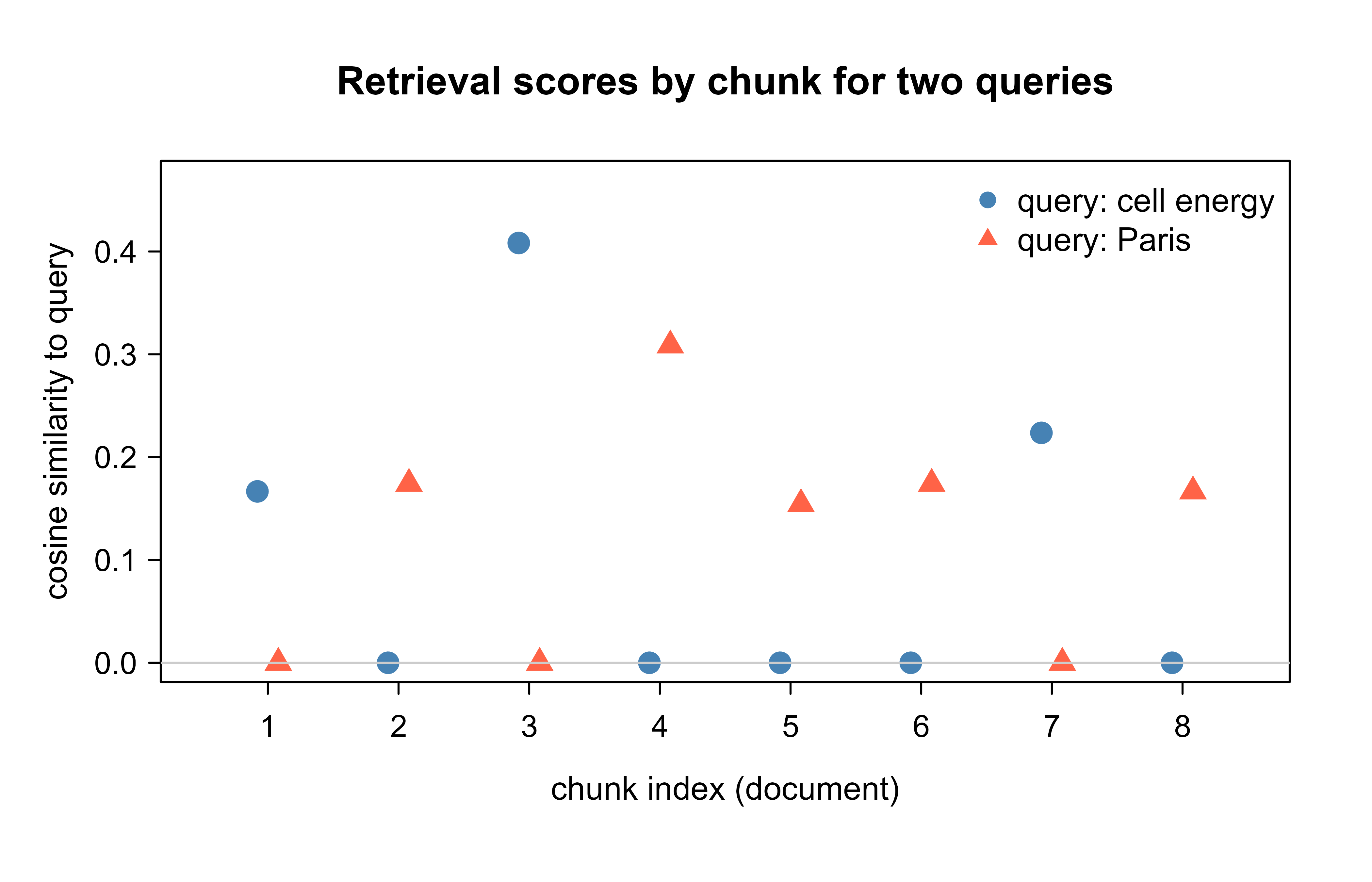
111.8.1 A Figure: Score Separation Across Queries

Figure 111.1 shows the retrieval scores of every chunk for two queries on different topics. A working retriever should separate the on-topic chunks (high score) from the off-topic ones (low score). The gap between the two groups is what makes top-$k$ selection reliable.

Show code

score_all <- function(query, E, vocab) {
    q <- l2_normalize(embed(query, vocab))
    as.numeric(E %*% q)
}

q1 <- "How do cells produce energy?"
q2 <- "What can you see in Paris France?"

s1 <- score_all(q1, E, vocab)
s2 <- score_all(q2, E, vocab)

m <- length(chunks)
plot(NA, xlim = c(0.5, m + 0.5), ylim = c(0, max(s1, s2) * 1.15),
     xlab = "chunk index (document)", ylab = "cosine similarity to query",
     main = "Retrieval scores by chunk for two queries", xaxt = "n")
axis(1, at = seq_len(m), labels = seq_len(m))
points(seq_len(m) - 0.08, s1, pch = 19, col = "steelblue", cex = 1.4)
points(seq_len(m) + 0.08, s2, pch = 17, col = "tomato", cex = 1.4)
abline(h = 0, col = "gray80")
legend("topright",
       legend = c("query: cell energy", "query: Paris"),
       pch = c(19, 17), col = c("steelblue", "tomato"), bty = "n")

Figure 111.1: Cosine retrieval scores for every chunk under two queries. Each query scores its on-topic chunks well above the rest, and the gap is what top-k selection exploits.

111.9 The Generation Step

With the top chunks retrieved, generation assembles the prompt and calls a language model. The call below uses the ellmer package, the current idiomatic way to talk to a chat model from R. It is marked eval=FALSE because it needs an external model and an API key, but it is correct code a reader can run after setting their credentials.

Note

This chunk does not run when the book builds because it depends on a live model endpoint and an API key, neither of which is available in the build environment. The retrieval code earlier in the chapter runs in plain base R precisely so the geometry can be demonstrated without any external service.

Show code

library(ellmer)

# Assemble labeled context from the retrieved chunks.
build_context <- function(top) {
    blocks <- sprintf("[source: %s]\n%s", top$source, top$chunk)
    paste(blocks, collapse = "\n\n")
}

context <- build_context(top)

system_prompt <- paste(
    "You answer questions using only the provided context.",
    "Cite the source tag for every claim, for example [source: doc3].",
    "If the answer is not in the context, reply that you do not know."
)

user_message <- paste0(
    "Context:\n", context, "\n\n",
    "Question: ", query, "\n\n",
    "Answer using only the context above and cite your sources."
)

chat <- chat_anthropic(system_prompt = system_prompt)
answer <- chat$chat(user_message)
cat(answer)

The instruction to cite sources and to abstain is what turns retrieved text into a grounded, auditable answer, and writing those instructions well is the subject of the prompt engineering chapter (Chapter 109). Everything upstream (chunking, embedding, retrieval, reranking) exists to make sure the context handed to this step actually contains the answer.

111.10 Evaluation

A RAG system has two parts to evaluate, and they fail independently. Retrieval can return the wrong chunks, or retrieval can succeed and generation can still produce a wrong answer. Measure them separately before measuring them end to end.

Tip

When an end-to-end answer is wrong, resist the urge to fix the prompt first. Check the retrieval metrics: if the right chunk never reached the model, no amount of prompt tuning will help. Isolating which stage failed is most of the debugging work.

Retrieval metrics treat retrieval as ranking against a set of known-relevant chunks per query. For a query whose relevant chunk is at rank $r$ in the returned list (or $\infty$ if not returned), two common measures are recall at $k$ and mean reciprocal rank,

\[ \text{Recall@}k = \frac{\#\{\text{relevant chunks in top } k\}}{\#\{\text{relevant chunks}\}}, \qquad \text{MRR} = \frac{1}{|Q|} \sum_{q \in Q} \frac{1}{r_q} , \]

where $Q$ is the set of evaluation queries and $r_q$ is the rank of the first relevant chunk for query $q$. Recall@$k$ asks whether the answer is in the candidate set at all (the first-stage job); MRR rewards putting it near the top (the reranker’s job).

Generation metrics assess the answer given the retrieved context. The two that matter most for RAG are faithfulness (every claim in the answer is supported by the retrieved context, which detects hallucination) and answer relevance (the answer addresses the question). These are often scored by an LLM-as-judge⁵: a separate model is prompted to check each claim against the context. Treat judge scores as noisy and validate them against a small human-labeled sample. Table 111.3 gathers the retrieval and generation metrics and pairs each one with the failure it detects.

Table 111.3: RAG evaluation metrics. Each metric measures one property of retrieval or generation and points to the specific failure mode it is designed to catch.

Metric	What it measures	Detects which failure
Recall@$k$	Relevant chunk is in the top $k$	First-stage retrieval miss
MRR / nDCG	Relevant chunk is ranked high	Weak reranking
Faithfulness	Claims are supported by context	Hallucination despite context
Answer relevance	Answer addresses the question	Off-topic or evasive answer
Abstention rate	Says “I do not know” when context lacks the answer	Ungrounded answering

Build the evaluation set from real queries plus their correct answers and supporting chunks, and include adversarial queries whose answers are deliberately absent from the corpus so the abstention rate is measurable.

111.11 Failure Modes and Practical Guidance

RAG fails in characteristic ways, and most production debugging is about locating which stage broke. The list below pairs each common failure with its likely cause, its fix, and the metric that detects it, so you can move from symptom to diagnosis quickly.

Retrieval miss. The right chunk was never returned, so the model had no chance. Causes: chunks too large (relevant sentence diluted), embedding model weak on the domain, dense-only retrieval missing an exact term. Fix with smaller or boundary-aligned chunks, hybrid retrieval, and a domain-appropriate embedding model. Diagnose with Recall@$k$.
Ranking miss. The right chunk was retrieved but ranked below the cutoff, so it never reached the prompt. Add or improve the reranker. Diagnose with MRR computed on the first-stage list.
Lost in the middle. The right chunk was in the context but buried where the model underuses it. Shorten the context and place strong chunks at the ends.
Hallucination despite context. The context contained the answer but the model answered from memory or invented detail. Strengthen the grounding instruction, require per-claim citations, and lower the temperature. Diagnose with faithfulness.
Failure to abstain. No relevant chunk exists but the model answers anyway. Make abstention explicit in the instruction and test it directly. Diagnose with abstention rate on absent-answer queries.
Stale index. Documents changed but the index was not rebuilt, so the system retrieves and cites outdated text. Treat re-indexing as a scheduled job tied to the document source.

When to use this

Use RAG when the knowledge is large, changing, or must be cited, and when you can keep an index fresh. Prefer fine-tuning when you need to change behavior or format rather than facts, and prefer plain long-context prompting when the reference material is small and fixed enough to paste into every request.

These three options are composable rather than mutually exclusive: a fine-tuned model that retrieves from a fresh index and abstains when the index comes up empty is a common and robust design. Stepping back, the whole pipeline in this chapter exists to serve one goal, putting true, relevant, citable text in front of the model at the moment it answers. Chunking, embedding, retrieval, and reranking decide what text arrives; grounding and citations decide how honestly the model uses it; and evaluation tells you which of those links is the weak one.

111.12 Further Reading

Lewis et al. (2020) introduced retrieval-augmented generation, combining a dense retriever with a sequence generator trained end to end.
Karpukhin et al. (2020) presented Dense Passage Retrieval, the bi-encoder approach behind most dense retrieval systems.
Robertson and Zaragoza (2009) gave the standard treatment of BM25 and probabilistic sparse retrieval, the basis of hybrid search.
Reimers and Gurevych (2019) introduced Sentence-BERT, the sentence-embedding and bi-encoder/cross-encoder framing used for retrieval and reranking.
Nogueira and Cho (2019) showed cross-encoder reranking of retrieved passages with a pretrained transformer.
Liu et al. (2024) documented the “lost in the middle” effect, showing how position in a long context changes how well a model uses retrieved information.
Es et al. (2024) proposed RAGAS, an automated evaluation framework for faithfulness and answer relevance in RAG systems.
Gao et al. (2023) surveyed retrieval-augmented generation for large language models, organizing the design space covered in this chapter.

A hallucination is a generated statement that is grammatical and confident but not supported by any source. The danger is that it reads exactly like a correct answer, so a reader cannot tell the two apart without checking.↩︎
A chunk is a contiguous span of a document, typically a paragraph or a few sentences, treated as one retrievable unit. A token is a sub-word unit the model counts in; for English text, plan on roughly four characters per token.↩︎
$k$ here is the number of chunks we keep. Choosing $k$ is a balance: too small and the right chunk may fall just outside the cut; too large and the prompt fills with marginal text. First-stage retrieval typically uses a generous $k$ (tens of candidates) and lets the reranker trim it down.↩︎
Abstention is the model declining to answer (saying “I do not know”) when the retrieved context does not contain the answer. It is the single clearest signal that a RAG system is actually reading its context rather than answering from memory.↩︎
LLM-as-judge means using a second language model to grade the first model’s output, for example to decide whether each claim is supported by the context. It scales far better than human grading but introduces its own biases, so calibrate it against human labels before trusting it.↩︎

# Retrieval-Augmented Generation (RAG) {#sec-retrieval-augmented-generation} ```{r} #| include: false source("_common.R") ``` Retrieval-augmented generation (RAG) is a pattern that gives a language model access to an external store of text at query time. Instead of relying only on what a model memorized during training, a RAG system first retrieves passages relevant to the user's question from a document collection, then passes those passages to the model as context and asks it to answer using them. The model still does the writing, but the facts come from documents you control. This pattern matters because the two failure modes of a bare language model are exactly the ones retrieval fixes. A model trained months ago does not know about events or documents created since, and a model asked about something it never saw will often produce a fluent but wrong answer (a hallucination^[A *hallucination* is a generated statement that is grammatical and confident but not supported by any source. The danger is that it reads exactly like a correct answer, so a reader cannot tell the two apart without checking.]). RAG addresses both: it keeps the knowledge in an updatable store outside the model, and it grounds the answer in retrieved text so the model has something true to copy from and to cite. ::: {.callout-tip title="Intuition"} Think of a bare language model as a smart student answering from memory in a closed-book exam, and a RAG system as the same student taking an open-book exam. The student is no more intelligent in the second case, but the answers are better because the relevant facts are sitting open on the desk. ::: This chapter covers the components of a RAG system in the order they run: chunking the documents, embedding the chunks, retrieving by similarity, reranking the candidates, assembling the context, and grounding the answer with citations. It then covers evaluation and the failure modes that show up in production. The retrieval step builds directly on the embeddings and dense-vector ideas from the embeddings and vector search chapter (@sec-embeddings-vector-search), and the generation step builds on the large language models chapter (@sec-llms). The runnable demonstration implements a minimal retriever in base R: cosine similarity over a small document set returning the top-$k$ chunks for a query. The generation call is shown as `eval=FALSE` because it requires an external model. ## Where This Fits in a Modern Workflow A data team usually has more proprietary text than any public model was trained on: support tickets, internal wikis, contracts, product manuals, research notes. Fine-tuning a model on all of it is slow, expensive, and goes stale the moment a document changes. RAG is the lighter-weight alternative. You index the text once, keep the index fresh as documents change, and the model reads from it on demand. No model weights move when a document is added or edited. ::: {.callout-important title="Key idea"} RAG separates *what the system knows* (the document index, which you own and can update freely) from *how the system writes* (the language model, whose weights stay fixed). Changing the facts no longer means retraining anything. ::: A RAG system has two phases. 1. Indexing (offline). Split documents into chunks, embed each chunk into a vector, and store the vectors in an index that supports fast nearest-neighbor search. This runs as a batch job and reruns when the corpus changes. 2. Serving (online). Embed the user's query with the same embedding model, retrieve the nearest chunks, optionally rerank them, assemble a prompt that contains the question and the retrieved chunks, and call the language model to produce a grounded answer with citations. The decision of RAG versus fine-tuning is not exclusive. Fine-tuning changes how a model behaves (tone, format, task skill); RAG changes what a model knows (facts, current documents). Teams often do both: fine-tune for the response style, retrieve for the facts. @tbl-retrieval-augmented-generation-rag-vs-finetune lays the three options side by side so you can see which lever each one pulls. | Property | RAG | Fine-tuning | Long-context prompting | |----|----|----|----| | Adds new facts | Yes, by updating the index | Yes, by retraining | Yes, paste documents in | | Update cost when a document changes | Re-embed one chunk | Retrain the model | None, but pay per token every call | | Provides citations | Yes, retrieved chunks are the source | No, source is not tracked | Possible if you ask | | Cost driver | Index storage and retrieval | Training compute | Tokens per request | | Best for | Large, changing knowledge bases | Stable task behavior and style | Small, fixed reference text | : Comparison of RAG, fine-tuning, and long-context prompting across the facts they add, their update cost, citation support, cost driver, and the setting each one suits best. {#tbl-retrieval-augmented-generation-rag-vs-finetune} ## Chunking A document is usually too long to retrieve or to fit in a prompt as a single unit, so it is split into chunks.^[A *chunk* is a contiguous span of a document, typically a paragraph or a few sentences, treated as one retrievable unit. A *token* is a sub-word unit the model counts in; for English text, plan on roughly four characters per token.] The chunk is the atomic unit of retrieval: the system retrieves chunks, scores chunks, and cites chunks. Chunk size is the first real design choice and it trades two errors against each other. Let a document have $L$ tokens. Split it into chunks of target size $c$ tokens with overlap $o$ tokens between consecutive chunks. The number of chunks is approximately $$ m \approx \left\lceil \frac{L - o}{c - o} \right\rceil . $$ Small chunks (a few sentences) give precise retrieval: a matching chunk is mostly relevant text, so the signal-to-noise ratio in the context is high. But a small chunk can be cut off from the context it needs, so an answer that spans two chunks gets split. Large chunks (a page) keep context together but dilute the match: a relevant sentence is surrounded by unrelated text, which lowers the similarity score and wastes prompt budget. The overlap $o$ exists so a sentence near a boundary still appears whole in at least one chunk. ::: {.callout-warning} Chunk size is not a setting you can guess once and forget. Too small and answers fragment across chunks; too large and the relevant sentence drowns in noise. It is one of the first knobs to tune against the evaluation set described later in the chapter. ::: In practice, split on natural boundaries (paragraphs, headings, list items) rather than at fixed token counts, so a chunk is a coherent unit of meaning. Typical settings are chunks of 200 to 500 tokens with 10 to 20 percent overlap, tuned against the evaluation set described later. Keep metadata with each chunk (source document, section, position) because that metadata becomes the citation. ## Embedding Once a document is chunked, each chunk has to become something a computer can compare for meaning, not just for shared words. That is the job of an embedding. The intuition is that we place every chunk as a point in a high-dimensional space, arranged so that chunks about the same idea land close together, and a query lands near the chunks that answer it. Retrieval then becomes "find the nearest points." More precisely, each chunk is mapped to a vector by an embedding model. An embedding is a function $f$ that maps a piece of text $t$ to a vector $f(t) \in \mathbb{R}^{d}$ such that texts with similar meaning map to nearby vectors. The same $f$ embeds the query and the chunks, so query and chunk live in the same space and can be compared directly. The construction and training of these models is the subject of the embeddings and vector search chapter (@sec-embeddings-vector-search); here we use the property that the geometry of the space encodes semantic similarity. The standard similarity is cosine similarity. For two vectors $u, v \in \mathbb{R}^{d}$, $$ \operatorname{cos}(u, v) = \frac{u^\top v}{\lVert u \rVert \, \lVert v \rVert} . $$ If the vectors are $\ell_2$-normalized so that $\lVert u \rVert = \lVert v \rVert = 1$, cosine similarity reduces to the dot product $u^\top v$, and the chunk that maximizes cosine similarity is the same one that minimizes squared Euclidean distance, since $$ \lVert u - v \rVert^2 = \lVert u \rVert^2 + \lVert v \rVert^2 - 2\, u^\top v = 2 - 2\, u^\top v $$ for unit vectors. This equivalence is why most vector stores normalize once at index time and then use the dot product, which is cheap. ::: {.callout-tip} Normalize every embedding to unit length the moment you compute it. After that, "most similar," "largest dot product," and "smallest Euclidean distance" all pick the same chunk, and the comparison reduces to one multiplication-and-sum. ::: Two embedding strategies are worth distinguishing, because the choice between them is the reason RAG has two retrieval stages rather than one. A bi-encoder embeds the query and each chunk separately, so all chunk vectors are precomputed at index time and retrieval is a fast similarity search. A cross-encoder takes the query and a chunk together and outputs a single relevance score; it is more accurate because it can attend across both texts (the attention mechanism is covered in @sec-transformers), but it cannot precompute anything and must run once per candidate. RAG uses the bi-encoder for the first-stage retrieval (fast, over the whole corpus) and reserves the cross-encoder for reranking a short candidate list, covered below. ::: {.callout-note} The bi-encoder is fast but reads the query and the chunk in isolation; the cross-encoder is slow but reads them together, so it can notice that a chunk answers *this exact* question. Keep this trade in mind: it is exactly why we retrieve cheaply over everything, then rerank expensively over a few. ::: ## Retrieval Retrieval finds the chunks whose embeddings are most similar to the query embedding. Let the corpus have $m$ chunks with normalized embeddings $e_1, \dots, e_m \in \mathbb{R}^{d}$ stacked as rows of a matrix $E \in \mathbb{R}^{m \times d}$, and let the query embedding be $q \in \mathbb{R}^{d}$, also normalized. The similarity scores are the single matrix-vector product $$ s = E q \in \mathbb{R}^{m}, \qquad s_i = e_i^\top q , $$ and the top-$k$ retrieval returns the indices of the $k$ largest entries of $s$.^[$k$ here is the number of chunks we keep. Choosing $k$ is a balance: too small and the right chunk may fall just outside the cut; too large and the prompt fills with marginal text. First-stage retrieval typically uses a generous $k$ (tens of candidates) and lets the reranker trim it down.] This exact search is $O(md)$ per query, which is fine for thousands of chunks but too slow for millions. Production systems use approximate nearest neighbor (ANN) indexes (graph-based methods such as HNSW, or quantization methods) that trade a small amount of recall for a large speedup. The math of the score does not change; only the search over $s$ becomes approximate. A purely dense (embedding-based) retriever can miss exact-match terms such as a product code or a rare name, because those carry little semantic signal but matter literally. The classical sparse retriever BM25 scores by term overlap and handles exact matches well. Hybrid retrieval combines the two, for example by summing a dense score and a sparse score after putting them on a comparable scale, $$ s_i^{\text{hybrid}} = \alpha \, s_i^{\text{dense}} + (1 - \alpha) \, s_i^{\text{sparse}}, \qquad \alpha \in [0, 1] , $$ with $\alpha$ tuned on the evaluation set. Hybrid retrieval is a strong default because the two retrievers fail on different queries. ::: {.callout-tip title="When to use this"} Reach for hybrid retrieval whenever your queries contain literal tokens that must match exactly: part numbers, error codes, function names, surnames, legal citations. Dense embeddings smooth meaning together, which is helpful for paraphrases but harmful when the user means *that specific string*. BM25 covers the gap. ::: ## Reranking First-stage retrieval is tuned for recall: return a candidate set of size $k$ (say 50) that probably contains the right chunk, accepting that the ordering within that set is rough. Reranking then reorders the candidates for precision using a stronger but slower model, and the top few after reranking go into the prompt. The reranker is typically a cross-encoder. For each candidate chunk $c_j$ in the retrieved set, it computes a relevance score $r_j = g(q, c_j)$ by reading the query and the chunk jointly, then the candidates are sorted by $r_j$. Because the cross-encoder reads both texts together it captures interactions a bi-encoder cannot, which is why a cheap recall-oriented first stage followed by an accurate reranker outperforms either alone. The cost is bounded because the cross-encoder runs only $k$ times per query, not $m$ times. ::: {.callout-tip title="Intuition"} The first stage casts a wide net to make sure the right chunk is somewhere in the haul; the reranker then sorts the haul carefully so the best chunk ends up on top. Doing both is cheaper than running the careful sort over the whole corpus and more accurate than trusting the wide net's rough ordering. ::: @tbl-retrieval-augmented-generation-two-stage contrasts the two stages on the model they use, the set they run over, what they optimize, and their cost. | Stage | Model type | Runs over | Optimized for | Cost per query | |----|----|----|----|----| | First-stage retrieval | Bi-encoder (plus BM25) | Whole corpus ($m$ chunks) | Recall | Low (precomputed vectors) | | Reranking | Cross-encoder | Candidate set ($k$ chunks) | Precision | Moderate ($k$ scorings) | : The two retrieval stages compared. First-stage retrieval runs a cheap bi-encoder over the whole corpus for recall, while reranking runs an accurate cross-encoder over the small candidate set for precision. {#tbl-retrieval-augmented-generation-two-stage} ## Context Assembly After reranking, the top chunks are assembled into the prompt. This step looks clerical but it determines what the model can actually use. Three constraints shape it. First, the context window is finite, so there is a token budget for retrieved chunks after accounting for the question, the instructions, and room for the answer. Pack the highest-ranked chunks until the budget is reached. Second, position matters. Models attend unevenly across a long context and tend to use information at the beginning and the end more than information buried in the middle, an effect documented as "lost in the middle." A practical response is to place the strongest chunks at the start and end of the context block, and to keep the context short rather than padding it with marginal chunks. ::: {.callout-warning} More context is not always better. Padding the prompt with marginal chunks can push the genuinely useful chunk into the middle, where the model is most likely to overlook it. A short, well-ordered context usually beats a long, exhaustive one. ::: Third, the chunks must be labeled so the model can cite them. Wrap each chunk with its source identifier, for example a tag like `[doc: handbook.pdf, section 3]`, and instruct the model to reference those identifiers. The assembled prompt has three parts: an instruction that tells the model to answer only from the provided context and to cite sources, the labeled chunks, and the user's question. ## Grounding and Citations Grounding means the answer is supported by the retrieved text rather than by the model's parametric memory. The instruction does part of the work ("answer using only the context below; if the answer is not there, say you do not know"), but instructions alone are not a guarantee. Two mechanisms make grounding checkable. The first is citation. Ask the model to attach, to each claim, the identifier of the chunk that supports it. A reader (or an automated check) can then verify each claim against its cited chunk. Citations turn an opaque answer into one whose provenance can be audited, which is often the reason RAG is chosen over fine-tuning in regulated settings. The second is abstention.^[*Abstention* is the model declining to answer (saying "I do not know") when the retrieved context does not contain the answer. It is the single clearest signal that a RAG system is actually reading its context rather than answering from memory.] The instruction to say "I do not know" when the context lacks the answer is what prevents the model from filling gaps with invented facts. A RAG system that never abstains is not grounded; it has merely added retrieved text to a model that still answers from memory when the retrieval misses. Measuring the abstention rate on queries whose answer is deliberately absent from the corpus is a direct test of grounding. ::: {.callout-important title="Key idea"} Grounding is not something you assert, it is something you can check. Citations let you verify each claim against its source, and abstention lets you confirm the model stays silent when no source supports an answer. A RAG system you cannot audit is not really grounded. ::: ## A Minimal RAG Retriever in Base R The demonstration implements the retrieval core: a small document set, a deterministic embedding so the example runs anywhere, cosine similarity, and top-$k$ selection. The embedding here is a simple bag-of-words vector over a fixed vocabulary, which is not a learned model but exercises exactly the same geometry (normalize, dot product, rank). A real system swaps this `embed()` for a call to an embedding model; nothing else in the pipeline changes. ```{r rag-corpus} # A tiny document set. Each entry is one chunk with a source label. chunks <- c( "The mitochondria is the powerhouse of the cell and produces ATP energy.", "Photosynthesis in plants converts sunlight carbon dioxide and water into glucose.", "ATP is the main energy currency used by cells for metabolic work.", "The capital of France is Paris which sits on the river Seine.", "Paris hosts many museums including the Louvre and the Musee d Orsay.", "Glucose produced by photosynthesis is stored as starch in plant tissue.", "Cellular respiration breaks down glucose to release energy as ATP.", "The river Seine flows through Paris toward the English Channel." ) sources <- paste0("doc", seq_along(chunks)) ``` ```{r rag-embed} # Build a fixed vocabulary from the corpus, then embed any text as a # bag-of-words count vector over that vocabulary. tokenize <- function(text) { text <- tolower(text) text <- gsub("[^a-z ]", " ", text) toks <- strsplit(text, "\\s+")[[1]] toks[nchar(toks) > 0] } vocab <- sort(unique(unlist(lapply(chunks, tokenize)))) embed <- function(text, vocab) { toks <- tokenize(text) v <- tabulate(match(toks, vocab), nbins = length(vocab)) as.numeric(v) } # l2-normalize a vector so cosine similarity becomes a dot product l2_normalize <- function(v) { n <- sqrt(sum(v^2)) if (n == 0) v else v / n } # Embed every chunk once at index time and stack as rows of E. E <- t(vapply(chunks, function(ch) l2_normalize(embed(ch, vocab)), numeric(length(vocab)))) dim(E) # m chunks by d vocabulary terms ``` ```{r rag-retrieve} # Retrieve the top-k chunks for a query by cosine similarity. retrieve <- function(query, E, chunks, sources, vocab, k = 3) { q <- l2_normalize(embed(query, vocab)) scores <- as.numeric(E %*% q) # s_i = e_i^T q ord <- order(scores, decreasing = TRUE)[seq_len(k)] data.frame( rank = seq_len(k), score = round(scores[ord], 3), source = sources[ord], chunk = chunks[ord], stringsAsFactors = FALSE ) } query <- "How do cells produce energy?" top <- retrieve(query, E, chunks, sources, vocab, k = 3) print(top[, c("rank", "score", "source")]) cat("\nTop chunk:\n", top$chunk[1], "\n") ``` The retriever ranks the energy and ATP chunks above the Paris chunks for an energy question, even though the query shares no rare words with some of the relevant chunks, because overlap on the common terms (energy, cells, produce) drives the cosine score. A learned embedding would do better on paraphrases (a query about "metabolism" with no shared words), but the ranking mechanism is identical. ### A Figure: Score Separation Across Queries @fig-retrieval-augmented-generation-score-separation shows the retrieval scores of every chunk for two queries on different topics. A working retriever should separate the on-topic chunks (high score) from the off-topic ones (low score). The gap between the two groups is what makes top-$k$ selection reliable. ```{r fig-retrieval-augmented-generation-score-separation, fig.width=7, fig.height=4.5, fig.cap="Cosine retrieval scores for every chunk under two queries. Each query scores its on-topic chunks well above the rest, and the gap is what top-k selection exploits."} score_all <- function(query, E, vocab) { q <- l2_normalize(embed(query, vocab)) as.numeric(E %*% q) } q1 <- "How do cells produce energy?" q2 <- "What can you see in Paris France?" s1 <- score_all(q1, E, vocab) s2 <- score_all(q2, E, vocab) m <- length(chunks) plot(NA, xlim = c(0.5, m + 0.5), ylim = c(0, max(s1, s2) * 1.15), xlab = "chunk index (document)", ylab = "cosine similarity to query", main = "Retrieval scores by chunk for two queries", xaxt = "n") axis(1, at = seq_len(m), labels = seq_len(m)) points(seq_len(m) - 0.08, s1, pch = 19, col = "steelblue", cex = 1.4) points(seq_len(m) + 0.08, s2, pch = 17, col = "tomato", cex = 1.4) abline(h = 0, col = "gray80") legend("topright", legend = c("query: cell energy", "query: Paris"), pch = c(19, 17), col = c("steelblue", "tomato"), bty = "n") ``` ## The Generation Step With the top chunks retrieved, generation assembles the prompt and calls a language model. The call below uses the `ellmer` package, the current idiomatic way to talk to a chat model from R. It is marked `eval=FALSE` because it needs an external model and an API key, but it is correct code a reader can run after setting their credentials. ::: {.callout-note} This chunk does not run when the book builds because it depends on a live model endpoint and an API key, neither of which is available in the build environment. The retrieval code earlier in the chapter runs in plain base R precisely so the geometry can be demonstrated without any external service. ::: ```{r rag-generate, eval=FALSE} library(ellmer) # Assemble labeled context from the retrieved chunks. build_context <- function(top) { blocks <- sprintf("[source: %s]\n%s", top$source, top$chunk) paste(blocks, collapse = "\n\n") } context <- build_context(top) system_prompt <- paste( "You answer questions using only the provided context.", "Cite the source tag for every claim, for example [source: doc3].", "If the answer is not in the context, reply that you do not know." ) user_message <- paste0( "Context:\n", context, "\n\n", "Question: ", query, "\n\n", "Answer using only the context above and cite your sources." ) chat <- chat_anthropic(system_prompt = system_prompt) answer <- chat$chat(user_message) cat(answer) ``` The instruction to cite sources and to abstain is what turns retrieved text into a grounded, auditable answer, and writing those instructions well is the subject of the prompt engineering chapter (@sec-prompt-engineering). Everything upstream (chunking, embedding, retrieval, reranking) exists to make sure the context handed to this step actually contains the answer. ## Evaluation A RAG system has two parts to evaluate, and they fail independently. Retrieval can return the wrong chunks, or retrieval can succeed and generation can still produce a wrong answer. Measure them separately before measuring them end to end. ::: {.callout-tip} When an end-to-end answer is wrong, resist the urge to fix the prompt first. Check the retrieval metrics: if the right chunk never reached the model, no amount of prompt tuning will help. Isolating which stage failed is most of the debugging work. ::: Retrieval metrics treat retrieval as ranking against a set of known-relevant chunks per query. For a query whose relevant chunk is at rank $r$ in the returned list (or $\infty$ if not returned), two common measures are recall at $k$ and mean reciprocal rank, $$ \text{Recall@}k = \frac{\#\{\text{relevant chunks in top } k\}}{\#\{\text{relevant chunks}\}}, \qquad \text{MRR} = \frac{1}{|Q|} \sum_{q \in Q} \frac{1}{r_q} , $$ where $Q$ is the set of evaluation queries and $r_q$ is the rank of the first relevant chunk for query $q$. Recall@$k$ asks whether the answer is in the candidate set at all (the first-stage job); MRR rewards putting it near the top (the reranker's job). Generation metrics assess the answer given the retrieved context. The two that matter most for RAG are faithfulness (every claim in the answer is supported by the retrieved context, which detects hallucination) and answer relevance (the answer addresses the question). These are often scored by an LLM-as-judge^[*LLM-as-judge* means using a second language model to grade the first model's output, for example to decide whether each claim is supported by the context. It scales far better than human grading but introduces its own biases, so calibrate it against human labels before trusting it.]: a separate model is prompted to check each claim against the context. Treat judge scores as noisy and validate them against a small human-labeled sample. @tbl-retrieval-augmented-generation-eval-metrics gathers the retrieval and generation metrics and pairs each one with the failure it detects. | Metric | What it measures | Detects which failure | |----|----|----| | Recall@$k$ | Relevant chunk is in the top $k$ | First-stage retrieval miss | | MRR / nDCG | Relevant chunk is ranked high | Weak reranking | | Faithfulness | Claims are supported by context | Hallucination despite context | | Answer relevance | Answer addresses the question | Off-topic or evasive answer | | Abstention rate | Says "I do not know" when context lacks the answer | Ungrounded answering | : RAG evaluation metrics. Each metric measures one property of retrieval or generation and points to the specific failure mode it is designed to catch. {#tbl-retrieval-augmented-generation-eval-metrics} Build the evaluation set from real queries plus their correct answers and supporting chunks, and include adversarial queries whose answers are deliberately absent from the corpus so the abstention rate is measurable. ## Failure Modes and Practical Guidance RAG fails in characteristic ways, and most production debugging is about locating which stage broke. The list below pairs each common failure with its likely cause, its fix, and the metric that detects it, so you can move from symptom to diagnosis quickly. - Retrieval miss. The right chunk was never returned, so the model had no chance. Causes: chunks too large (relevant sentence diluted), embedding model weak on the domain, dense-only retrieval missing an exact term. Fix with smaller or boundary-aligned chunks, hybrid retrieval, and a domain-appropriate embedding model. Diagnose with Recall@$k$. - Ranking miss. The right chunk was retrieved but ranked below the cutoff, so it never reached the prompt. Add or improve the reranker. Diagnose with MRR computed on the first-stage list. - Lost in the middle. The right chunk was in the context but buried where the model underuses it. Shorten the context and place strong chunks at the ends. - Hallucination despite context. The context contained the answer but the model answered from memory or invented detail. Strengthen the grounding instruction, require per-claim citations, and lower the temperature. Diagnose with faithfulness. - Failure to abstain. No relevant chunk exists but the model answers anyway. Make abstention explicit in the instruction and test it directly. Diagnose with abstention rate on absent-answer queries. - Stale index. Documents changed but the index was not rebuilt, so the system retrieves and cites outdated text. Treat re-indexing as a scheduled job tied to the document source. ::: {.callout-tip title="When to use this"} Use RAG when the knowledge is large, changing, or must be cited, and when you can keep an index fresh. Prefer fine-tuning when you need to change behavior or format rather than facts, and prefer plain long-context prompting when the reference material is small and fixed enough to paste into every request. ::: These three options are composable rather than mutually exclusive: a fine-tuned model that retrieves from a fresh index and abstains when the index comes up empty is a common and robust design. Stepping back, the whole pipeline in this chapter exists to serve one goal, putting true, relevant, citable text in front of the model at the moment it answers. Chunking, embedding, retrieval, and reranking decide *what* text arrives; grounding and citations decide *how honestly* the model uses it; and evaluation tells you which of those links is the weak one. ## Further Reading - Lewis et al. (2020) introduced retrieval-augmented generation, combining a dense retriever with a sequence generator trained end to end. - Karpukhin et al. (2020) presented Dense Passage Retrieval, the bi-encoder approach behind most dense retrieval systems. - Robertson and Zaragoza (2009) gave the standard treatment of BM25 and probabilistic sparse retrieval, the basis of hybrid search. - Reimers and Gurevych (2019) introduced Sentence-BERT, the sentence-embedding and bi-encoder/cross-encoder framing used for retrieval and reranking. - Nogueira and Cho (2019) showed cross-encoder reranking of retrieved passages with a pretrained transformer. - Liu et al. (2024) documented the "lost in the middle" effect, showing how position in a long context changes how well a model uses retrieved information. - Es et al. (2024) proposed RAGAS, an automated evaluation framework for faithfulness and answer relevance in RAG systems. - Gao et al. (2023) surveyed retrieval-augmented generation for large language models, organizing the design space covered in this chapter.