Probabilistic programming is a way of writing statistical models as code. You declare how the data are generated from unknown parameters and what you believe about those parameters before seeing data, and the system handles the inference: turning the model plus the observed data into a posterior distribution over the parameters. Stan is one of the most widely used probabilistic programming systems, and brms and rstanarm are R packages that let you specify Stan models through the familiar R formula interface.
This chapter explains the idea, the sampling machinery (Markov chain Monte Carlo, Hamiltonian Monte Carlo, and the No-U-Turn Sampler), how priors and posteriors fit together, how to check a fitted model with posterior predictive checks, and how the formula interface in brms and rstanarm maps to Stan code. Because Stan and brms are not installed in this environment, those code chunks are shown with eval=FALSE but are written so a reader can run them directly. The runnable demonstration is a small Metropolis-Hastings sampler written in base R, which exposes the core mechanics that Stan automates.
Intuition
A traditional model hands you a single best guess for each parameter. A probabilistic model hands you the full set of guesses that are still plausible after seeing the data, weighted by how plausible each one is. Everything in this chapter is machinery for producing and inspecting that weighted set of guesses, called the posterior.
When to use this
Reach for probabilistic programming when the deliverable is uncertainty itself, a credible interval, a calibrated forecast, or a probability statement a decision-maker can act on, rather than a single number. If all you need is the most accurate point prediction on a large dataset, a method from earlier chapters will usually be faster.
75.1 Where this fits in a modern ML and AI workflow
Most supervised learning methods in this book return a point prediction or a point estimate of parameters. A probabilistic model returns a full distribution. For a regression coefficient you get not a single number but a posterior distribution that summarizes every value consistent with the data and the prior.1 For a prediction at a new input you get a predictive distribution, not just a mean.
This matters in practice when:
You need calibrated uncertainty, for example a credible interval on a treatment effect, a risk score that feeds a decision, or a forecast that downstream code must reason about probabilistically.
You have hierarchical or grouped data (students within schools, measurements within patients, sales within stores), where partial pooling across groups improves estimates for small groups.
You want to encode domain knowledge as priors, for example bounding a rate to be positive or shrinking coefficients toward zero in a principled way.
The likelihood is custom or non-standard, so off-the-shelf estimators do not exist.
In an ML or AI pipeline, probabilistic models often sit at the layer where decisions are made under uncertainty: A/B test analysis, demand forecasting, sensor fusion, and Bayesian optimization of hyperparameters (Chapter 84). They are usually slower to fit than gradient-boosted trees or neural networks and are not the right tool for very large feature spaces with no structure, but they are hard to beat when uncertainty and interpretability are the deliverable.
75.2 The probabilistic programming idea
A probabilistic program describes a joint distribution over parameters \(\theta\) and data \(y\):
The denominator \(p(y)\), called the marginal likelihood or evidence, is an integral over all of parameter space. For most models it has no closed form, and that integral is what makes Bayesian inference hard. The central trick of modern probabilistic programming is that we almost never need \(p(y)\) to draw samples from the posterior. Because
an algorithm that only needs the posterior up to a constant can ignore \(p(y)\) entirely. Markov chain Monte Carlo (MCMC) is exactly such an algorithm: it produces a sequence of parameter draws whose stationary distribution is the posterior, using only the unnormalized product \(p(y \mid \theta) \, p(\theta)\).
Key idea
Because the posterior is proportional to likelihood times prior, and the only missing piece, \(p(y)\), is a constant that does not depend on \(\theta\), any sampler that works with ratios or gradients of the posterior can skip the hard integral entirely. This single observation is what makes Bayesian computation practical.
A probabilistic programming language separates the model from the inference. You write the model (priors and likelihood), and the system compiles it and runs a general-purpose sampler. Stan compiles your model to C++ and runs an adaptive Hamiltonian Monte Carlo sampler. You do not derive update equations by hand.2
The rest of the chapter follows the natural order of a Bayesian analysis: first the samplers that explore the posterior, then how priors and likelihood combine into that posterior, then a worked example you can run, then how to check the fit, and finally the tools that let you write all of this with a one-line formula.
75.3 MCMC, HMC, and NUTS intuition
Since we cannot compute the posterior in closed form, we draw samples from it instead. A histogram of enough samples is as good as the density itself for any practical summary: a mean, a quantile, a credible interval. The samplers below differ only in how cleverly they wander through parameter space to produce those samples. We build up from the simplest idea to the one Stan actually uses.
75.3.1 Metropolis-Hastings
The simplest MCMC method is the Metropolis-Hastings (MH) algorithm. Let \(\pi(\theta) \propto p(y \mid \theta) \, p(\theta)\) be the unnormalized posterior. Starting from a current point \(\theta\), propose a candidate \(\theta^*\) from a proposal distribution \(q(\theta^* \mid \theta)\), then accept the candidate with probability
If the proposal is symmetric, meaning \(q(\theta^* \mid \theta) = q(\theta \mid \theta^*)\) (a Gaussian centered at the current point is the usual choice), the ratio simplifies to \(\alpha = \min(1, \pi(\theta^*)/\pi(\theta))\). Notice that the normalizing constant \(p(y)\) cancels in the ratio, so only the unnormalized posterior appears. After many steps and a burn-in period,3 the retained draws behave like samples from \(p(\theta \mid y)\).
Intuition
Think of MH as exploring a hilly landscape in the dark, where height is posterior probability. From where you stand you take a random step. If it leads uphill you always take it; if it leads downhill you take it only sometimes, more often for a gentle slope than a cliff. Over time you spend the most time where the landscape is highest, which is exactly the posterior.
MH is simple but can be slow. If the proposal steps are too small the chain explores slowly; if too large most proposals are rejected. In high dimensions a random-walk proposal wanders inefficiently, and the number of steps needed to get an effectively independent sample grows quickly.
75.3.1.1 Why Metropolis-Hastings targets the posterior
The acceptance rule above is not arbitrary: it is the unique choice that makes the posterior the stationary distribution of the chain. The standard sufficient condition is detailed balance (reversibility) with respect to the target \(\pi\). A transition kernel \(P(\theta \to \theta')\) satisfies detailed balance if
for all \(\theta, \theta'\). Integrating Equation 75.1 over \(\theta\) gives \(\int \pi(\theta) P(\theta \to \theta')\, d\theta = \pi(\theta') \int P(\theta' \to \theta)\, d\theta = \pi(\theta')\), which is exactly the statement that \(\pi\) is invariant: one step started from \(\pi\) leaves the distribution unchanged.
For MH the off-diagonal part of the kernel (the probability of actually moving from \(\theta\) to \(\theta' \ne \theta\)) is the proposal density times the acceptance probability, \(P(\theta \to \theta') = q(\theta' \mid \theta)\, \alpha(\theta, \theta')\). Substitute the MH acceptance probability \(\alpha(\theta,\theta') = \min\!\big(1,\, \tfrac{\pi(\theta') q(\theta \mid \theta')}{\pi(\theta) q(\theta' \mid \theta)}\big)\) and check Equation 75.1. Without loss of generality suppose the ratio \(\tfrac{\pi(\theta') q(\theta \mid \theta')}{\pi(\theta) q(\theta' \mid \theta)} \le 1\), so \(\alpha(\theta,\theta') = \tfrac{\pi(\theta') q(\theta \mid \theta')}{\pi(\theta) q(\theta' \mid \theta)}\) and the reverse move has \(\alpha(\theta',\theta) = 1\). Then
which is Equation 75.1. The case where the ratio exceeds one is symmetric. Two points are worth drawing out. First, \(\pi\) appears only through the ratio \(\pi(\theta')/\pi(\theta)\), so the normalizing constant \(p(y)\) cancels exactly, which is the formal version of the “key idea” callout above. Second, detailed balance plus irreducibility (the chain can reach any region of positive posterior mass) and aperiodicity guarantee that the chain converges to \(\pi\) from any starting point; this is the ergodic theorem that justifies discarding warmup and averaging the rest.
Optimal scaling of random-walk MH
For a target made of \(d\) independent and identically distributed coordinates and a Gaussian proposal \(\mathcal{N}(\theta, \ell^2 \Sigma / d)\), Roberts, Gelman, and Gilks (1997) showed that as \(d \to \infty\) the efficiency of random-walk MH is maximized when the proposal scale is tuned so that the acceptance rate approaches \(0.234\). This is the theoretical basis for the rule of thumb that random-walk acceptance should land in the rough range \(0.2\) to \(0.5\) used in the demo. The same analysis shows the number of steps to produce one effectively independent draw grows linearly in \(d\), the curse of dimensionality that motivates the gradient-based samplers below.
75.3.2 Hamiltonian Monte Carlo
Hamiltonian Monte Carlo (HMC) reduces random-walk behavior by using gradient information. It augments the parameters \(\theta\) with auxiliary momentum variables \(r\) of the same dimension, and defines a joint density
Here \(U(\theta)\) is the potential energy (the negative log posterior) and the quadratic term in \(r\) is the kinetic energy with mass matrix \(M\). HMC simulates the physics of a particle moving across the posterior surface by integrating Hamilton’s equations, usually with the leapfrog integrator, for a number of steps, then proposes the endpoint. Because the trajectory follows the gradient of the log posterior, proposals can travel far across the distribution while still being accepted with high probability. This is why HMC needs the gradient \(\nabla_\theta \log p(\theta \mid y)\), which Stan computes automatically by reverse-mode automatic differentiation.4
Intuition
Instead of taking blind random steps, HMC gives the explorer a sense of the local slope and a push of momentum, so it skis along the contours of the landscape. One trajectory can cross to a far corner of the posterior in a single proposal, which is why HMC mixes so much faster than random-walk MH in high dimensions.
75.3.2.1 Why HMC works: Hamiltonian dynamics and the acceptance correction
The joint density in \((\theta, r)\) defines a Hamiltonian, the total energy,
so that the joint target is \(p(\theta, r) \propto \exp(-H(\theta, r))\). The momentum is auxiliary: because \(H\) separates additively and \(r \sim \mathcal{N}(0, M)\) is independent of \(\theta\), marginalizing out \(r\) returns the posterior, \(\int p(\theta, r)\, dr \propto \exp(-U(\theta)) = p(y\mid\theta)p(\theta)\). So if we can sample the joint \((\theta, r)\) and then discard \(r\), the \(\theta\) draws are exactly posterior draws.
The continuous-time dynamics follow Hamilton’s equations,
Exact Hamiltonian flow has three properties that make it an ideal proposal mechanism. First it conserves energy: \(\tfrac{dH}{dt} = \nabla_\theta H \cdot \dot\theta + \nabla_r H \cdot \dot r = \nabla_\theta U \cdot M^{-1} r - M^{-1} r \cdot \nabla_\theta U = 0\), so a trajectory stays on a level set of \(H\) where the joint density is constant and the proposal would always be accepted. Second it preserves volume in \((\theta, r)\) space (Liouville’s theorem), because the flow field has zero divergence: \(\sum_i \tfrac{\partial}{\partial \theta_i}\tfrac{\partial H}{\partial r_i} + \sum_i \tfrac{\partial}{\partial r_i}\big(-\tfrac{\partial H}{\partial \theta_i}\big) = 0\). Third it is time-reversible. Volume preservation means the proposal carries no Jacobian factor, and reversibility lets us keep detailed balance.
In practice we cannot solve Equation 75.3 exactly, so Stan uses the leapfrog (Stormer-Verlet) integrator, which for step size \(\epsilon\) takes a half momentum step, a full position step, and a half momentum step:
Each leapfrog substep is a shear (it updates one block using only the other), so each has unit Jacobian and the whole map is volume preserving exactly, even though it only approximates the true flow. The leapfrog map is also exactly reversible: negating the momentum, applying \(L\) steps, and negating again returns the start. What it does not do is conserve \(H\) exactly; it conserves it to second order, with error \(O(\epsilon^2)\) per step that does not accumulate without bound (the integrator is symplectic). The small energy error is precisely what the Metropolis accept step corrects. After \(L\) leapfrog steps from \((\theta, r)\) to \((\theta^*, r^*)\), propose with acceptance probability
Because the leapfrog map is volume preserving and reversible, this is an ordinary Metropolis correction on the joint space and it leaves \(\exp(-H)\) invariant exactly, so the marginal over \(\theta\) is the exact posterior despite the discretization error. One full HMC iteration is therefore: draw fresh momentum \(r \sim \mathcal{N}(0, M)\), run \(L\) leapfrog steps, and accept or reject by Equation 75.5. Resampling \(r\) each iteration is what lets the chain change energy levels and explore the whole posterior rather than a single level set.
Cost, scaling, and the mass matrix
HMC’s advantage is quantitative. Under suitable conditions Neal (2011) and Beskos et al. (2013) show that to keep the acceptance rate fixed as dimension grows, the step size must scale like \(\epsilon \propto d^{-1/4}\), so the number of leapfrog steps for one effectively independent draw scales like \(d^{1/4}\), versus \(d\) for random-walk MH and \(d^{1/2}\) for the Metropolis-adjusted Langevin algorithm. The optimal acceptance rate for HMC under this analysis is about \(0.65\), which is why Stan’s default adapt_delta is \(0.8\) and not the \(0.234\) of random-walk MH. The mass matrix \(M\) plays the role of a preconditioner: choosing \(M\) close to the inverse posterior covariance makes the target isotropic in the transformed coordinates and dramatically improves mixing. Stan estimates a diagonal (or dense) \(M\) from the warmup draws for exactly this reason, which is why correlated parameters are handled “well, mass matrix adapted in warmup” in Table 75.1.
75.3.3 The No-U-Turn Sampler
HMC has two tuning parameters: the leapfrog step size \(\epsilon\) and the number of steps \(L\). Choosing \(L\) by hand is awkward: too few steps and the sampler behaves like a random walk, too many and it wastes computation by looping back on itself. The No-U-Turn Sampler (NUTS) automatically chooses the trajectory length by extending the path until it starts to double back (a “U-turn”), and Stan adapts \(\epsilon\) during warmup. NUTS is the default sampler in Stan, brms, and rstanarm, which is why these tools usually work well with little manual tuning.
Tip
In day-to-day work you almost never tune the sampler by hand. The payoff of NUTS is that you can focus on the model (the priors and likelihood) and trust the defaults for inference, stepping in only when the diagnostics later in the chapter flag a problem.
Table 75.1: Comparison of Metropolis-Hastings, Hamiltonian Monte Carlo, and the No-U-Turn Sampler across gradient use, tuning, scaling behavior, and typical use.
Property
Metropolis-Hastings
Hamiltonian Monte Carlo
NUTS
Uses gradient of log posterior
No
Yes
Yes
Tuning required
Proposal scale
Step size and number of steps
Step size and number of steps adapted automatically
Behavior in high dimensions
Random walk, slow mixing
Long informed moves
Long informed moves
Handles correlated parameters
Poorly without tuning
Well with a tuned mass matrix
Well, mass matrix adapted in warmup
Implementation effort
Low
Moderate
Built into Stan
Typical use
Teaching, simple models
Foundation for modern samplers
Default in Stan, brms, rstanarm
75.4 Priors and posteriors
With the samplers in hand, we can step back to the two pieces you actually have to specify: the prior and the likelihood. The sampler is plumbing; the prior and likelihood are the model.
The prior \(p(\theta)\) encodes what you believe about parameters before seeing the data. Choices range across a spectrum, from priors that carry strong information to those that carry almost none:
Informative priors carry real domain knowledge, for example a prior on a reaction rate that must be positive and is known to be near a literature value.
Weakly informative priors rule out absurd values while staying broad, for example a \(\text{Normal}(0, 2.5^2)\) prior on a standardized regression coefficient. These are the recommended default in rstanarm and a common choice in brms.
Flat or improper priors carry almost no information and can cause poor sampling or improper posteriors, so they are usually avoided.
The posterior combines prior and likelihood. With more data the likelihood dominates and the prior matters less; with little data the prior matters more. A useful identity for intuition is the conjugate Gaussian case. Suppose \(y_1, \dots, y_n\) are independent \(\text{Normal}(\mu, \sigma^2)\) with known \(\sigma^2\), and the prior is \(\mu \sim \text{Normal}(\mu_0, \tau^2)\). Then the posterior is Gaussian with
The posterior mean is a precision-weighted average of the prior mean \(\mu_0\) and the data mean \(\bar{y}\), where precision is the reciprocal of variance. As \(n\) grows, the data term \(n/\sigma^2\) dominates and the posterior concentrates near \(\bar{y}\). This closed form is the exception; for general models we sample instead, which is the subject of the demo below.
75.4.0.1 Deriving the conjugate Gaussian posterior
The identity above follows from completing the square in the log posterior, the prototype of every conjugate update. Dropping additive constants that do not depend on \(\mu\), the unnormalized log posterior is the log likelihood plus the log prior,
using \(\sum_i y_i = n\bar y\). Any function of the form \(-\tfrac{1}{2}A\mu^2 + B\mu + \text{const}\) is, up to a constant, the log density of a Gaussian: completing the square gives \(-\tfrac{A}{2}\big(\mu - B/A\big)^2 + \text{const}\), which is \(\mathcal{N}(B/A,\, A^{-1})\). Reading off the mean and variance,
which is exactly the stated result. The structure generalizes: posterior precision is the sum of prior precision and data precision (\(A = \tau^{-2} + n\sigma^{-2}\)), and the posterior mean is the precision-weighted average of the two information sources. This additivity of precisions is the formal content of the statement that priors and data combine, and it is why a weakly informative prior (small \(\tau^{-2}\)) is quickly dominated once \(n\) is moderate.
The following short check confirms the closed form against a brute-force numerical posterior on a grid, using only base R.
Show code
set.seed(11)sigma2<-4; tau2<-9; mu0<-1# known data var, prior var, prior meanyv<-rnorm(25, mean =3, sd =sqrt(sigma2))# data from mu = 3n<-length(yv); ybar<-mean(yv)# Closed-form posterior (the derived formulas)post_var<-1/(1/tau2+n/sigma2)post_mean<-post_var*(mu0/tau2+n*ybar/sigma2)# Numerical posterior on a fine grid (unnormalized -> normalized)grid<-seq(post_mean-6*sqrt(post_var), post_mean+6*sqrt(post_var), length =4000)logpost<-sapply(grid, function(m)sum(dnorm(yv, m, sqrt(sigma2), log =TRUE))+dnorm(m, mu0, sqrt(tau2), log =TRUE))w<-exp(logpost-max(logpost)); w<-w/sum(w)num_mean<-sum(grid*w)num_var<-sum((grid-num_mean)^2*w)round(c(closed_mean =post_mean, grid_mean =num_mean, closed_var =post_var, grid_var =num_var), 4)#> closed_mean grid_mean closed_var grid_var #> 2.3593 2.3593 0.1572 0.1572
The closed-form mean and variance match the grid-based posterior to several decimals, confirming the completing-the-square derivation.
Note
A 95 percent credible interval, the central 95 percent of the posterior, says there is a 95 percent probability the parameter lies in that range given the model and data. That is a direct probability statement about the parameter, which is not what a frequentist confidence interval claims. The distinction is worth keeping straight when you report results.
75.5 A runnable Metropolis-Hastings demo in base R
Stan and brms automate everything we have discussed, which can make the machinery feel like a black box. To dispel that, the following demo implements the whole loop by hand in about a dozen lines: it fits a logistic regression with two parameters (intercept and slope) to simulated binary data, using a hand-written random-walk Metropolis-Hastings sampler. It uses only base R, so it runs here. The model is
We work on the log scale for numerical stability.5 The log posterior is the log likelihood plus the log prior, up to the constant \(\log p(y)\) that MH does not need.
Show code
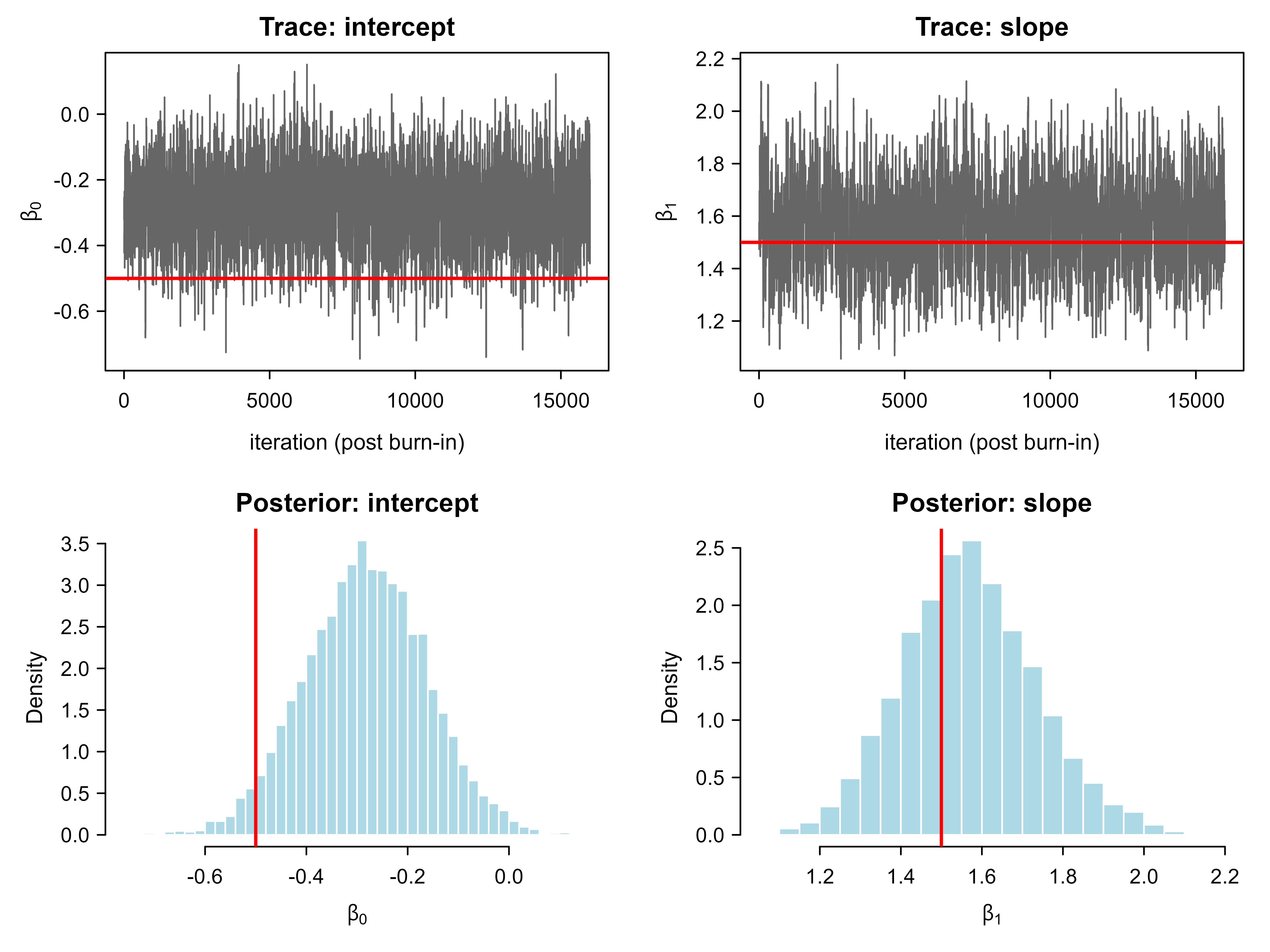
set.seed(1301)# Simulate data from a known logistic modeln<-400x<-rnorm(n)beta_true<-c(-0.5, 1.5)# intercept, slopeeta<-beta_true[1]+beta_true[2]*xp<-1/(1+exp(-eta))y<-rbinom(n, size =1, prob =p)# Unnormalized log posterior: log-likelihood + log-priorlog_posterior<-function(beta, x, y, prior_sd=5){eta<-beta[1]+beta[2]*x# numerically stable Bernoulli log-likelihoodloglik<-sum(y*eta-log1p(exp(eta)))logprior<-sum(dnorm(beta, mean =0, sd =prior_sd, log =TRUE))loglik+logprior}# Random-walk Metropolis-Hastings with a symmetric Gaussian proposalmetropolis<-function(log_post, init, n_iter, proposal_sd, ...){p<-length(init)draws<-matrix(NA_real_, nrow =n_iter, ncol =p)current<-initcurrent_lp<-log_post(current, ...)n_accept<-0for(tinseq_len(n_iter)){candidate<-current+rnorm(p, mean =0, sd =proposal_sd)cand_lp<-log_post(candidate, ...)# symmetric proposal so the acceptance ratio is the posterior ratiolog_alpha<-cand_lp-current_lpif(log(runif(1))<log_alpha){current<-candidatecurrent_lp<-cand_lpn_accept<-n_accept+1}draws[t, ]<-current}list(draws =draws, accept_rate =n_accept/n_iter)}n_iter<-20000fit<-metropolis(log_posterior, init =c(0, 0), n_iter =n_iter, proposal_sd =0.12, x =x, y =y)# Discard a burn-in period, then summarizeburnin<-4000post<-fit$draws[(burnin+1):n_iter, ]colnames(post)<-c("beta0", "beta1")cat(sprintf("Acceptance rate: %.2f\n", fit$accept_rate))#> Acceptance rate: 0.61post_summary<-t(apply(post, 2, function(z)c(mean =mean(z), sd =sd(z), q2.5 =quantile(z, 0.025), q97.5 =quantile(z, 0.975))))print(round(post_summary, 3))#> mean sd q2.5.2.5% q97.5.97.5%#> beta0 -0.283 0.120 -0.519 -0.048#> beta1 1.570 0.165 1.258 1.911# Figure: trace plots and posterior histogramsop<-par(mfrow =c(2, 2), mar =c(4, 4, 2, 1))plot(post[, "beta0"], type ="l", col ="grey40", xlab ="iteration (post burn-in)", ylab =expression(beta[0]), main ="Trace: intercept")abline(h =beta_true[1], col ="red", lwd =2)plot(post[, "beta1"], type ="l", col ="grey40", xlab ="iteration (post burn-in)", ylab =expression(beta[1]), main ="Trace: slope")abline(h =beta_true[2], col ="red", lwd =2)hist(post[, "beta0"], breaks =40, col ="lightblue", border ="white", xlab =expression(beta[0]), main ="Posterior: intercept", freq =FALSE)abline(v =beta_true[1], col ="red", lwd =2)hist(post[, "beta1"], breaks =40, col ="lightblue", border ="white", xlab =expression(beta[1]), main ="Posterior: slope", freq =FALSE)abline(v =beta_true[2], col ="red", lwd =2)par(op)
Figure 75.1: Metropolis-Hastings output for a two-parameter logistic regression: trace plots (top) and posterior histograms with true values marked (bottom).
Reading the output in words: Figure 75.1 shows the trace plots, which should look like stationary noise with no drift, a sign the chain has converged and is mixing. In the same figure the posterior histograms concentrate around the true coefficients (the red lines), and the 2.5 and 97.5 percent quantiles give a 95 percent credible interval for each parameter. A random-walk sampler typically mixes best with an acceptance rate somewhere between about 0.2 and 0.5; if the rate is very high the steps are too small and the chain crawls, and if very low most proposals are wasted, so in either case you would retune proposal_sd. Stan replaces this manual tuning with adaptive NUTS, but the underlying logic (propose, compare unnormalized posteriors, accept or reject) is the same.
Warning
This base R sampler is for teaching, not production. It uses a single chain, a fixed proposal scale, and no automatic warmup adaptation. For any real analysis use Stan through brms or rstanarm, which run multiple chains, adapt the sampler, and report the diagnostics covered later in this chapter.
As a quick sanity check, the posterior means should sit close to the maximum likelihood fit, since the prior here is weak relative to 400 observations.
Show code
glm_fit<-glm(y~x, family =binomial())round(coef(glm_fit), 3)# compare with posterior means above#> (Intercept) x #> -0.280 1.549
75.6 Posterior predictive checks
Fitting a model is not the same as trusting it. A posterior predictive check (PPC) asks whether data simulated from the fitted model look like the data you actually observed.
Key idea
A model that fits well should be able to regenerate data that resembles what you saw. If you simulate fake datasets from the fitted model and they look systematically different from the real one, the model is missing something, no matter how clean the parameter estimates look.
In practice you draw \(\theta^{(s)}\) from the posterior, then draw a replicated dataset \(y^{\text{rep},(s)} \sim p(y^{\text{rep}} \mid \theta^{(s)})\) for each draw. You then compare summaries of \(y^{\text{rep}}\) to the same summary of \(y\). If the observed summary is far in the tail of the replicated summaries, the model is missing something.
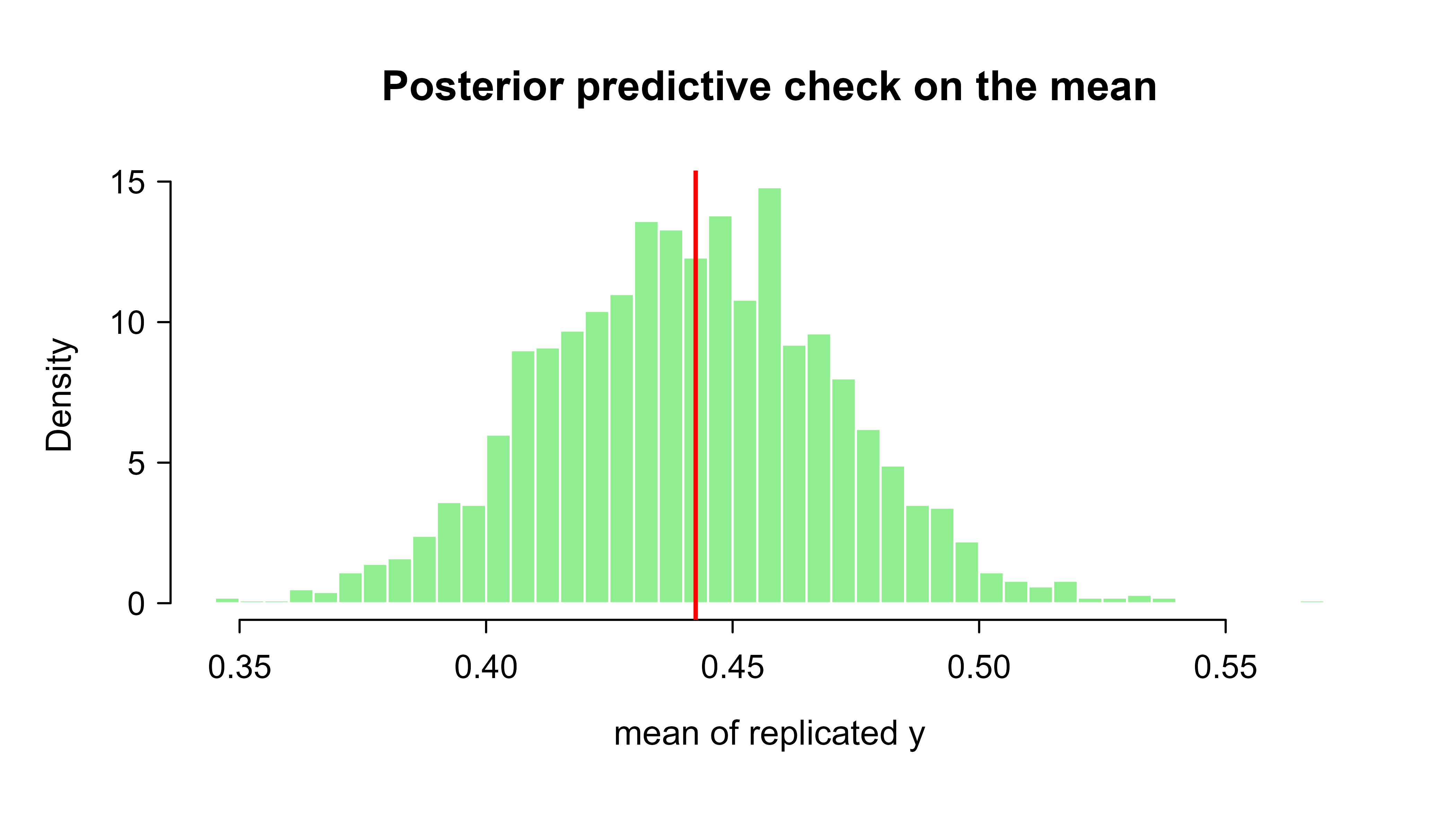
We can run a simple PPC with the base-R logistic fit from the demo. A reasonable test statistic for binary data is the proportion of ones in subgroups, or here the overall mean and its spread across replications. Figure 75.2 shows the result.
Show code
set.seed(7)S<-2000idx<-sample(nrow(post), S, replace =TRUE)# posterior draws to userep_means<-numeric(S)for(sinseq_len(S)){b<-post[idx[s], ]eta_s<-b[1]+b[2]*xp_s<-1/(1+exp(-eta_s))y_rep<-rbinom(length(x), size =1, prob =p_s)rep_means[s]<-mean(y_rep)}obs_mean<-mean(y)ppc_p<-mean(rep_means>=obs_mean)# a Bayesian posterior predictive p-valuehist(rep_means, breaks =40, col ="lightgreen", border ="white", xlab ="mean of replicated y", freq =FALSE, main ="Posterior predictive check on the mean")abline(v =obs_mean, col ="red", lwd =2)cat(sprintf("Observed mean: %.3f\n", obs_mean))#> Observed mean: 0.442cat(sprintf("Posterior predictive p-value: %.3f\n", ppc_p))#> Posterior predictive p-value: 0.515
Figure 75.2: Posterior predictive check: distribution of the replicated mean response across posterior draws, with the observed mean (red).
A posterior predictive p-value near 0.5 means the observed statistic sits in the middle of what the model predicts, which is what we want.6 Values very close to 0 or 1 flag misfit. In real workflows you would check several statistics (means within subgroups, variance, the count of zeros, residual patterns), not just one.
75.7 The brms and rstanarm formula interface
Now that you have seen the mechanics from the inside, here is how you would do all of this in practice without writing a sampler at all. Writing Stan by hand is flexible but verbose. brms and rstanarm let you specify common models with R formulas and generate the Stan code for you. They differ in approach: rstanarm ships precompiled Stan models for standard families (faster to start, fixed menu), while brms writes and compiles fresh Stan code for each model (slower first run, far more flexible, supports custom families, nonlinear terms, multivariate responses, and distributional regression).
When to use this
Start with rstanarm if your model fits its menu of standard families, because it skips compilation and runs immediately. Reach for brms when you need something beyond that menu: a custom likelihood, a nonlinear formula, several response variables at once, or a model of the variance itself.
The next chunk shows the same logistic regression as the demo, fit with brms. It is eval=FALSE because brms and its Stan toolchain are not installed here, but the code is correct and current.
Show code
library(brms)dat<-data.frame(y =y, x =x)fit_brms<-brm( formula =y~x, data =dat, family =bernoulli(link ="logit"), prior =c(prior(normal(0, 5), class ="Intercept"),prior(normal(0, 5), class ="b")), chains =4, iter =2000, warmup =1000, cores =4, seed =1301, backend ="cmdstanr"# or the default "rstan")summary(fit_brms)# posterior means, SDs, 95% credible intervals, Rhat, ESSplot(fit_brms)# trace plots and density plots per parameterpp_check(fit_brms)# built-in posterior predictive checkconditional_effects(fit_brms)# fitted curve with credible band
The rstanarm equivalent uses a drop-in replacement for glm:
The formula interface really pays off for hierarchical (multilevel) models, where brms uses the same (term | group) syntax as lme4. The next example fits varying intercepts and slopes by group, which would be tedious to code by hand in raw Stan.
Show code
library(brms)# y_ij ~ Normal(mu_ij, sigma), mu_ij = (b0 + u0_j) + (b1 + u1_j) * x_ij# with group-level effects u0_j, u1_j drawn from a multivariate normalfit_h<-brm(y~x+(1+x|group), data =my_grouped_data, family =gaussian(), prior =c(prior(normal(0, 5), class ="b"),prior(student_t(3, 0, 2.5), class ="sd"), # group SDsprior(lkj(2), class ="cor")), # correlation of u0, u1 chains =4, iter =2000, cores =4, seed =1)# Inspect convergence and group-level estimatessummary(fit_h)ranef(fit_h)# estimated group deviationsloo(fit_h)# leave-one-out cross-validation for model comparison
For reference, the raw Stan program behind the simple logistic model looks like the block below. Reading it once makes clear what brms generates for you: a data block, a parameters block, a model block with priors and likelihood, and optionally a generated quantities block for predictions. This is Stan code, not R, so it is eval=FALSE.
Show code
stan_program<-"data { int<lower=0> N; vector[N] x; array[N] int<lower=0, upper=1> y;}parameters { real beta0; real beta1;}model { beta0 ~ normal(0, 5); beta1 ~ normal(0, 5); y ~ bernoulli_logit(beta0 + beta1 * x); // vectorized likelihood}generated quantities { array[N] int y_rep = bernoulli_logit_rng(beta0 + beta1 * x);}"# library(rstan); mod <- stan_model(model_code = stan_program)# fit <- sampling(mod, data = list(N = length(y), x = x, y = y))
75.8 Diagnostics you should always check
After sampling, never read the posterior summaries without first checking that the sampler worked. A beautiful-looking posterior mean from a chain that never converged is worse than useless, because it looks authoritative while being wrong. The standard diagnostics are summarized in Table 75.2.
Warning
Treat the diagnostics as a gate, not an afterthought. If \(\hat{R}\) is high or there are divergent transitions, the numbers in your summary table are not estimates of the posterior, and no amount of careful interpretation will fix that. Diagnose and refit first.
Table 75.2: Standard MCMC diagnostics, what each one measures, a healthy target value, and what a bad value indicates.
Diagnostic
What it measures
Healthy value
What a bad value means
\(\hat{R}\) (R-hat)
Agreement across chains for each parameter
\(\le 1.01\)
Chains have not converged to the same distribution
Effective sample size (ESS)
Number of effectively independent draws
At least a few hundred per parameter
High autocorrelation, summaries are noisy
Divergent transitions
Leapfrog steps that fail in HMC/NUTS
Zero, or very few
The sampler cannot explore part of the posterior; estimates may be biased
Trace plots
Visual mixing across iterations
“Fuzzy caterpillar”, overlapping chains
Drift, stuck chains, or multimodality
Energy diagnostic (BFMI)
Quality of momentum resampling in HMC
Above about 0.2
Heavy-tailed posterior the sampler handles poorly
In brms and rstanarm these appear in summary() output (Rhat, Bulk_ESS, Tail_ESS) and through bayesplot functions such as mcmc_trace(), mcmc_rank_overlay(), and mcmc_nuts_divergence(). Divergent transitions often signal a posterior with sharp geometry, common in hierarchical models; the usual fixes are raising adapt_delta (for example to 0.95 or 0.99), reparameterizing (the non-centered parameterization for group effects), or tightening overly vague priors.
75.8.1 Monte Carlo error, effective sample size, and \(\hat R\)
The diagnostics above are not heuristics bolted on after the fact; they estimate the actual error of the posterior summaries. For a function \(g(\theta)\) with posterior mean \(\mu_g = \mathbb{E}[g(\theta)\mid y]\), the MCMC estimator from \(N\) retained draws is \(\hat\mu_g = \tfrac{1}{N}\sum_{t=1}^{N} g(\theta^{(t)})\). The ergodic theorem gives \(\hat\mu_g \to \mu_g\) almost surely, but the draws are correlated, so the variance of the estimator is not \(\sigma_g^2 / N\). Writing \(\sigma_g^2 = \text{Var}(g(\theta))\) and \(\rho_k\) for the lag-\(k\) autocorrelation of the chain, the standard stationary-process variance is
The quantity \(N_{\text{eff}}\) is the effective sample size: the integrated autocorrelation time \(\tau_{\text{int}} = 1 + 2\sum_{k\ge 1}\rho_k\) tells you how many correlated draws are worth one independent draw. Positive autocorrelation (\(\rho_k > 0\)) inflates \(\tau_{\text{int}}\) and shrinks \(N_{\text{eff}}\) below \(N\); the Monte Carlo standard error of a posterior mean is then \(\widehat{\text{se}} = \hat\sigma_g / \sqrt{N_{\text{eff}}}\), which is why an ESS of a few hundred is the floor for a stable summary and more is needed for extreme tail quantiles. HMC and NUTS keep \(\rho_k\) small (the long informed moves decorrelate quickly), which is the practical reason they need so many fewer iterations than random-walk MH for the same precision.
The \(\hat R\) statistic compares between-chain and within-chain variance to detect non-convergence. With \(m\) chains each of length \(N\), posterior draws \(\theta^{(t)}_j\), chain means \(\bar\theta_j\), and grand mean \(\bar\theta\), define
\[
B = \frac{N}{m-1}\sum_{j=1}^{m}(\bar\theta_j - \bar\theta)^2, \qquad
W = \frac{1}{m}\sum_{j=1}^{m} s_j^2, \qquad s_j^2 = \frac{1}{N-1}\sum_{t=1}^{N}(\theta^{(t)}_j - \bar\theta_j)^2.
\]
The pooled marginal posterior variance is estimated by a weighted average of within and between variance, \(\widehat{\text{Var}}^+ = \tfrac{N-1}{N}W + \tfrac{1}{N}B\), and
\[
\hat R = \sqrt{\frac{\widehat{\text{Var}}^+}{W}}.
\tag{75.7}\]
If the chains have converged to the same stationary distribution, \(B\) and \(W\) estimate the same variance, \(\widehat{\text{Var}}^+ \approx W\), and \(\hat R \to 1\) as \(N \to \infty\). Values above \(1.01\) mean the between-chain spread still exceeds what the within-chain mixing would predict, so the chains are exploring different regions and have not converged. Running multiple chains from dispersed starts is what makes \(B\) informative; a single chain cannot reveal this failure, which is the formal reason the practical guidance recommends at least four chains. Modern implementations (the posterior package, used internally by brms and rstanarm) use a rank-normalized, split-chain version of Equation 75.7 that also catches a chain stuck in one mode and differences in scale, but the logic is the same.
75.9 Approximate inference and model comparison
MCMC returns asymptotically exact posterior draws but can be too slow on large data. Two further tools round out the workflow: a faster approximate sampler, and a principled way to compare fitted models.
75.9.1 Variational inference as an optimization problem
Variational inference (VI), exposed in brms and rstanarm through algorithm = "meanfield" or "fullrank", replaces sampling with optimization. Pick a tractable family of distributions \(q_\phi(\theta)\) indexed by parameters \(\phi\) (for mean-field, a product of independent Gaussians, \(q_\phi(\theta) = \prod_j \mathcal{N}(\theta_j; m_j, s_j^2)\)), and find the member closest to the posterior in Kullback-Leibler divergence:
We cannot evaluate this KL directly because it contains the intractable \(\log p(y)\). The standard maneuver is to expand it and isolate that constant:
is the evidence lower bound (ELBO). Since \(\log p(y)\) does not depend on \(\phi\), minimizing the KL is identical to maximizing the ELBO, and because KL is non-negative, Equation 75.8 is a lower bound on the log evidence, \(\mathcal{L}(\phi) \le \log p(y)\). Stan maximizes \(\mathcal{L}\) by stochastic gradient ascent, estimating \(\nabla_\phi \mathcal{L}\) with draws from \(q_\phi\) (the reparameterization trick writes \(\theta = m + s\odot\varepsilon\), \(\varepsilon\sim\mathcal{N}(0,I)\), so the gradient passes through the sampling step), which is exactly the automatic differentiation variational inference (ADVI) of Kucukelbir et al. (2017). VI is fast and scales to large data, but it has a systematic failure mode that the chapter’s earlier warning names: because KL\((q\|p)\) penalizes placing mass where the posterior is small far more than the reverse, the optimizer prefers a \(q\) that sits inside the posterior, so VI typically underestimates posterior variance and ignores correlations under the mean-field factorization. Use it for exploration or when MCMC is infeasible, then confirm critical uncertainty quantities with NUTS.
75.9.2 Predictive model comparison: WAIC and LOO
To compare models without overfitting to in-sample fit, the target is the expected log pointwise predictive density on new data, estimated through the posterior. The widely applicable information criterion (WAIC) estimates it from the fitted draws as
the log pointwise predictive density minus an effective-parameter penalty given by the posterior variance of the pointwise log likelihood. Leave-one-out cross-validation (LOO) targets the same quantity, \(\sum_i \log p(y_i \mid y_{-i})\), and the loo package computes it without refitting \(n\) times by importance sampling: the leave-one-out predictive uses importance weights \(w_i^{(s)} \propto 1/p(y_i\mid\theta^{(s)})\) applied to the full-data posterior draws. Raw importance weights have heavy tails, so loo fits a generalized Pareto distribution to the largest weights and reports the shape parameter \(\hat k\) as a diagnostic; \(\hat k < 0.7\) indicates the LOO estimate for that observation is reliable, and large \(\hat k\) flags an influential point where you should refit. PSIS-LOO is generally preferred to WAIC because its \(\hat k\) diagnostic warns you when the approximation breaks, whereas WAIC fails silently. Both compare models on the difference in elpd along with its standard error; a difference smaller than a couple of standard errors is not decisive.
75.10 Practical guidance, pitfalls, and when to use it
Having seen the idea, the samplers, a worked example, and the tooling, the remaining question is judgment: when is this approach the right one, and what trips people up. The following lists collect that practical advice. Start with the case for using probabilistic programming:
You need honest uncertainty intervals, not just point predictions.
You have hierarchical or grouped structure and want partial pooling.
Sample sizes are small to moderate and priors can stabilize estimates.
The likelihood is custom, or you want to combine several data sources in one coherent model.
Interpretability and the ability to state probability claims about parameters matter to stakeholders.
There are also clear cases where another method serves you better:
Very large datasets with millions of rows and no special structure: MCMC can be too slow, and a regularized GLM, gradient-boosted trees, or a neural network is usually faster and just as accurate for point prediction. Variational inference (brms with algorithm = "meanfield" or "fullrank") is an approximate, faster alternative when full MCMC is too expensive, at the cost of underestimated uncertainty.
Pure point-prediction tasks with no need for calibrated uncertainty.
Real-time, low-latency scoring, unless you precompute and cache the posterior.
Finally, a handful of mistakes account for most of the trouble newcomers run into:
Ignoring diagnostics. High \(\hat{R}\) or divergent transitions mean the summaries are not trustworthy no matter how reasonable they look.
Flat priors by default. They can produce improper posteriors and poor sampling. Prefer weakly informative priors and check sensitivity by refitting with a different prior.
Unscaled predictors. Default priors assume predictors are on a roughly standardized scale; center and scale continuous predictors so default priors behave as intended.
Too few iterations or chains. Run at least 4 chains and enough iterations that the effective sample size is comfortable, especially for tail quantiles.
Reading credible intervals as confidence intervals. A 95 percent credible interval is a direct probability statement about the parameter given the model and data, which is a different (and usually more intuitive) object than a frequentist confidence interval.
Overfitting model complexity. Use leave-one-out cross-validation (loo) or WAIC to compare models rather than chasing the lowest in-sample error.
Tip
A reasonable default recipe for a new analysis: standardize predictors, start from rstanarm or brms defaults with weakly informative priors, run 4 chains, check \(\hat{R}\), ESS, and divergences, run pp_check, then refine priors and structure and compare with loo. Treat this loop, fit, check, refine, as the normal workflow rather than a one-shot fit.
To sum up, probabilistic programming lets you write a generative model as code and get back a full posterior, with the hard inference handled by an adaptive sampler you rarely have to tune. The cost is computation and the discipline of checking diagnostics and predictive fit; the payoff is calibrated uncertainty and the ability to make direct probability statements about the quantities you care about.
75.11 Further reading
Gelman, Carlin, Stern, Dunson, Vehtari, and Rubin (2013), Bayesian Data Analysis, third edition, for the foundations of Bayesian modeling and model checking.
McElreath (2020), Statistical Rethinking, second edition, for an accessible, code-first introduction that pairs well with brms.
Neal (2011), “MCMC using Hamiltonian dynamics”, in the Handbook of Markov Chain Monte Carlo, for the canonical treatment of HMC.
Roberts, Gelman, and Gilks (1997), “Weak convergence and optimal scaling of random walk Metropolis algorithms”, in the Annals of Applied Probability, for the \(0.234\) optimal acceptance rate.
Beskos, Pillai, Roberts, Sanz-Serna, and Stuart (2013), “Optimal tuning of the hybrid Monte Carlo algorithm”, in Bernoulli, for the \(d^{1/4}\) scaling and the \(0.65\) optimal acceptance rate of HMC.
Kucukelbir, Tran, Ranganath, Gelman, and Blei (2017), “Automatic differentiation variational inference”, in the Journal of Machine Learning Research, for the VI algorithm behind Stan’s meanfield and fullrank modes.
Vehtari, Gelman, and Gabry (2017), “Practical Bayesian model evaluation using leave-one-out cross-validation and WAIC”, in Statistics and Computing, for PSIS-LOO and the \(\hat k\) diagnostic.
Hoffman and Gelman (2014), “The No-U-Turn Sampler”, in the Journal of Machine Learning Research, for the NUTS algorithm.
Carpenter, Gelman, Hoffman, Lee, Goodrich, Betancourt, Brubaker, Guo, Li, and Riddell (2017), “Stan: A Probabilistic Programming Language”, in the Journal of Statistical Software, for the Stan system.
Bürkner (2017), “brms: An R Package for Bayesian Multilevel Models Using Stan”, in the Journal of Statistical Software, for the brms formula interface.
Gabry, Simpson, Vehtari, Betancourt, and Gelman (2019), “Visualization in Bayesian workflow”, in the Journal of the Royal Statistical Society Series A, for posterior predictive checks and diagnostics.
The same shift in mindset shows up in Gaussian process regression (Chapter 7) and Bayesian additive regression trees (BART, Chapter 14) elsewhere in this book: those methods also return distributions rather than points. Probabilistic programming generalizes the idea to any model you can write down.↩︎
This separation is the same design principle that makes SQL useful (Chapter 99): you declare what you want, and an engine figures out how to compute it. Here you declare the generative model, and the sampler figures out how to explore the posterior.↩︎
Burn-in (also called warmup) is the initial stretch of draws produced before the chain settles into the posterior. Those early draws still reflect the arbitrary starting point, so we discard them.↩︎
Automatic differentiation, the same technique that powers backpropagation in neural networks (Chapter 15), computes exact gradients of the log posterior from the model code without you writing any derivatives by hand.↩︎
Probabilities of many data points multiply together into numbers so small they underflow to zero in floating-point arithmetic. Adding log-probabilities instead of multiplying probabilities keeps the computation in a safe numeric range, which is why nearly all probabilistic code works on the log scale.↩︎
This is not a frequentist p-value and there is no 0.05 threshold to pass. It simply locates the observed statistic within the distribution the model predicts; only values near 0 or 1 are a warning sign.↩︎
Source Code
# Probabilistic Programming with Stan and brms {#sec-probabilistic-programming}```{r}#| include: falsesource("_common.R")```Probabilistic programming is a way of writing statistical models as code. You declare how the data are generated from unknown parameters and what you believe about those parameters before seeing data, and the system handles the inference: turning the model plus the observed data into a posterior distribution over the parameters. Stan is one of the most widely used probabilistic programming systems, and `brms` and `rstanarm` are R packages that let you specify Stan models through the familiar R formula interface.This chapter explains the idea, the sampling machinery (Markov chain Monte Carlo, Hamiltonian Monte Carlo, and the No-U-Turn Sampler), how priors and posteriors fit together, how to check a fitted model with posterior predictive checks, and how the formula interface in `brms` and `rstanarm` maps to Stan code. Because Stan and `brms` are not installed in this environment, those code chunks are shown with `eval=FALSE` but are written so a reader can run them directly. The runnable demonstration is a small Metropolis-Hastings sampler written in base R, which exposes the core mechanics that Stan automates.::: {.callout-tip title="Intuition"}A traditional model hands you a single best guess for each parameter. A probabilistic model hands you the full set of guesses that are still plausible after seeing the data, weighted by how plausible each one is. Everything in this chapter is machinery for producing and inspecting that weighted set of guesses, called the posterior.:::::: {.callout-tip title="When to use this"}Reach for probabilistic programming when the deliverable is uncertainty itself, a credible interval, a calibrated forecast, or a probability statement a decision-maker can act on, rather than a single number. If all you need is the most accurate point prediction on a large dataset, a method from earlier chapters will usually be faster.:::## Where this fits in a modern ML and AI workflowMost supervised learning methods in this book return a point prediction or a point estimate of parameters. A probabilistic model returns a full distribution. For a regression coefficient you get not a single number but a posterior distribution that summarizes every value consistent with the data and the prior.^[The same shift in mindset shows up in Gaussian process regression (@sec-gaussian-process-reg) and Bayesian additive regression trees (BART, @sec-bart) elsewhere in this book: those methods also return distributions rather than points. Probabilistic programming generalizes the idea to any model you can write down.] For a prediction at a new input you get a predictive distribution, not just a mean.This matters in practice when:- You need calibrated uncertainty, for example a credible interval on a treatment effect, a risk score that feeds a decision, or a forecast that downstream code must reason about probabilistically.- You have hierarchical or grouped data (students within schools, measurements within patients, sales within stores), where partial pooling across groups improves estimates for small groups.- You want to encode domain knowledge as priors, for example bounding a rate to be positive or shrinking coefficients toward zero in a principled way.- The likelihood is custom or non-standard, so off-the-shelf estimators do not exist.In an ML or AI pipeline, probabilistic models often sit at the layer where decisions are made under uncertainty: A/B test analysis, demand forecasting, sensor fusion, and Bayesian optimization of hyperparameters (@sec-hyperparameter-optimization). They are usually slower to fit than gradient-boosted trees or neural networks and are not the right tool for very large feature spaces with no structure, but they are hard to beat when uncertainty and interpretability are the deliverable.## The probabilistic programming ideaA probabilistic program describes a joint distribution over parameters $\theta$ and data $y$:$$p(\theta, y) = p(y \mid \theta) \, p(\theta)$$where $p(\theta)$ is the prior and $p(y \mid \theta)$ is the likelihood. The goal of inference is the posterior, given by Bayes' rule:$$p(\theta \mid y) = \frac{p(y \mid \theta) \, p(\theta)}{p(y)}, \qquadp(y) = \int p(y \mid \theta) \, p(\theta) \, d\theta$$The denominator $p(y)$, called the marginal likelihood or evidence, is an integral over all of parameter space. For most models it has no closed form, and that integral is what makes Bayesian inference hard. The central trick of modern probabilistic programming is that we almost never need $p(y)$ to draw samples from the posterior. Because$$p(\theta \mid y) \propto p(y \mid \theta) \, p(\theta)$$an algorithm that only needs the posterior up to a constant can ignore $p(y)$ entirely. Markov chain Monte Carlo (MCMC) is exactly such an algorithm: it produces a sequence of parameter draws whose stationary distribution is the posterior, using only the unnormalized product $p(y \mid \theta) \, p(\theta)$.::: {.callout-important title="Key idea"}Because the posterior is proportional to likelihood times prior, and the only missing piece, $p(y)$, is a constant that does not depend on $\theta$, any sampler that works with ratios or gradients of the posterior can skip the hard integral entirely. This single observation is what makes Bayesian computation practical.:::A probabilistic programming language separates the model from the inference. You write the model (priors and likelihood), and the system compiles it and runs a general-purpose sampler. Stan compiles your model to C++ and runs an adaptive Hamiltonian Monte Carlo sampler. You do not derive update equations by hand.^[This separation is the same design principle that makes SQL useful (@sec-databases-sql-r): you declare what you want, and an engine figures out how to compute it. Here you declare the generative model, and the sampler figures out how to explore the posterior.]The rest of the chapter follows the natural order of a Bayesian analysis: first the samplers that explore the posterior, then how priors and likelihood combine into that posterior, then a worked example you can run, then how to check the fit, and finally the tools that let you write all of this with a one-line formula.## MCMC, HMC, and NUTS intuitionSince we cannot compute the posterior in closed form, we draw samples from it instead. A histogram of enough samples is as good as the density itself for any practical summary: a mean, a quantile, a credible interval. The samplers below differ only in how cleverly they wander through parameter space to produce those samples. We build up from the simplest idea to the one Stan actually uses.### Metropolis-HastingsThe simplest MCMC method is the Metropolis-Hastings (MH) algorithm. Let $\pi(\theta) \propto p(y \mid \theta) \, p(\theta)$ be the unnormalized posterior. Starting from a current point $\theta$, propose a candidate $\theta^*$ from a proposal distribution $q(\theta^* \mid \theta)$, then accept the candidate with probability$$\alpha = \min\left(1, \; \frac{\pi(\theta^*) \, q(\theta \mid \theta^*)}{\pi(\theta) \, q(\theta^* \mid \theta)}\right)$$If the proposal is symmetric, meaning $q(\theta^* \mid \theta) = q(\theta \mid \theta^*)$ (a Gaussian centered at the current point is the usual choice), the ratio simplifies to $\alpha = \min(1, \pi(\theta^*)/\pi(\theta))$. Notice that the normalizing constant $p(y)$ cancels in the ratio, so only the unnormalized posterior appears. After many steps and a burn-in period,^[Burn-in (also called warmup) is the initial stretch of draws produced before the chain settles into the posterior. Those early draws still reflect the arbitrary starting point, so we discard them.] the retained draws behave like samples from $p(\theta \mid y)$.::: {.callout-tip title="Intuition"}Think of MH as exploring a hilly landscape in the dark, where height is posterior probability. From where you stand you take a random step. If it leads uphill you always take it; if it leads downhill you take it only sometimes, more often for a gentle slope than a cliff. Over time you spend the most time where the landscape is highest, which is exactly the posterior.:::MH is simple but can be slow. If the proposal steps are too small the chain explores slowly; if too large most proposals are rejected. In high dimensions a random-walk proposal wanders inefficiently, and the number of steps needed to get an effectively independent sample grows quickly.#### Why Metropolis-Hastings targets the posteriorThe acceptance rule above is not arbitrary: it is the unique choice that makes the posterior the stationary distribution of the chain. The standard sufficient condition is *detailed balance* (reversibility) with respect to the target $\pi$. A transition kernel $P(\theta \to \theta')$ satisfies detailed balance if$$\pi(\theta) \, P(\theta \to \theta') = \pi(\theta') \, P(\theta' \to \theta)$$ {#eq-probabilistic-programming-detailed-balance}for all $\theta, \theta'$. Integrating @eq-probabilistic-programming-detailed-balance over $\theta$ gives $\int \pi(\theta) P(\theta \to \theta')\, d\theta = \pi(\theta') \int P(\theta' \to \theta)\, d\theta = \pi(\theta')$, which is exactly the statement that $\pi$ is invariant: one step started from $\pi$ leaves the distribution unchanged.For MH the off-diagonal part of the kernel (the probability of actually moving from $\theta$ to $\theta' \ne \theta$) is the proposal density times the acceptance probability, $P(\theta \to \theta') = q(\theta' \mid \theta)\, \alpha(\theta, \theta')$. Substitute the MH acceptance probability $\alpha(\theta,\theta') = \min\!\big(1,\, \tfrac{\pi(\theta') q(\theta \mid \theta')}{\pi(\theta) q(\theta' \mid \theta)}\big)$ and check @eq-probabilistic-programming-detailed-balance. Without loss of generality suppose the ratio $\tfrac{\pi(\theta') q(\theta \mid \theta')}{\pi(\theta) q(\theta' \mid \theta)} \le 1$, so $\alpha(\theta,\theta') = \tfrac{\pi(\theta') q(\theta \mid \theta')}{\pi(\theta) q(\theta' \mid \theta)}$ and the reverse move has $\alpha(\theta',\theta) = 1$. Then$$\pi(\theta)\, q(\theta' \mid \theta)\, \alpha(\theta,\theta')= \pi(\theta)\, q(\theta' \mid \theta) \cdot \frac{\pi(\theta')\, q(\theta \mid \theta')}{\pi(\theta)\, q(\theta' \mid \theta)}= \pi(\theta')\, q(\theta \mid \theta')= \pi(\theta')\, q(\theta \mid \theta')\, \alpha(\theta',\theta),$$which is @eq-probabilistic-programming-detailed-balance. The case where the ratio exceeds one is symmetric. Two points are worth drawing out. First, $\pi$ appears only through the ratio $\pi(\theta')/\pi(\theta)$, so the normalizing constant $p(y)$ cancels exactly, which is the formal version of the "key idea" callout above. Second, detailed balance plus irreducibility (the chain can reach any region of positive posterior mass) and aperiodicity guarantee that the chain converges to $\pi$ from any starting point; this is the ergodic theorem that justifies discarding warmup and averaging the rest.::: {.callout-note title="Optimal scaling of random-walk MH"}For a target made of $d$ independent and identically distributed coordinates and a Gaussian proposal $\mathcal{N}(\theta, \ell^2 \Sigma / d)$, Roberts, Gelman, and Gilks (1997) showed that as $d \to \infty$ the efficiency of random-walk MH is maximized when the proposal scale is tuned so that the acceptance rate approaches $0.234$. This is the theoretical basis for the rule of thumb that random-walk acceptance should land in the rough range $0.2$ to $0.5$ used in the demo. The same analysis shows the number of steps to produce one effectively independent draw grows linearly in $d$, the curse of dimensionality that motivates the gradient-based samplers below.:::### Hamiltonian Monte CarloHamiltonian Monte Carlo (HMC) reduces random-walk behavior by using gradient information. It augments the parameters $\theta$ with auxiliary momentum variables $r$ of the same dimension, and defines a joint density$$p(\theta, r) \propto \exp\left(-U(\theta) - \tfrac{1}{2} r^\top M^{-1} r\right), \qquad U(\theta) = -\log\big(p(y \mid \theta)\, p(\theta)\big)$$Here $U(\theta)$ is the potential energy (the negative log posterior) and the quadratic term in $r$ is the kinetic energy with mass matrix $M$. HMC simulates the physics of a particle moving across the posterior surface by integrating Hamilton's equations, usually with the leapfrog integrator, for a number of steps, then proposes the endpoint. Because the trajectory follows the gradient of the log posterior, proposals can travel far across the distribution while still being accepted with high probability. This is why HMC needs the gradient $\nabla_\theta \log p(\theta \mid y)$, which Stan computes automatically by reverse-mode automatic differentiation.^[Automatic differentiation, the same technique that powers backpropagation in neural networks (@sec-neural-networks), computes exact gradients of the log posterior from the model code without you writing any derivatives by hand.]::: {.callout-tip title="Intuition"}Instead of taking blind random steps, HMC gives the explorer a sense of the local slope and a push of momentum, so it skis along the contours of the landscape. One trajectory can cross to a far corner of the posterior in a single proposal, which is why HMC mixes so much faster than random-walk MH in high dimensions.:::#### Why HMC works: Hamiltonian dynamics and the acceptance correctionThe joint density in $(\theta, r)$ defines a Hamiltonian, the total energy,$$H(\theta, r) = U(\theta) + K(r), \qquad U(\theta) = -\log\big(p(y \mid \theta)\, p(\theta)\big), \quad K(r) = \tfrac{1}{2} r^\top M^{-1} r,$$ {#eq-probabilistic-programming-hamiltonian}so that the joint target is $p(\theta, r) \propto \exp(-H(\theta, r))$. The momentum is auxiliary: because $H$ separates additively and $r \sim \mathcal{N}(0, M)$ is independent of $\theta$, marginalizing out $r$ returns the posterior, $\int p(\theta, r)\, dr \propto \exp(-U(\theta)) = p(y\mid\theta)p(\theta)$. So if we can sample the joint $(\theta, r)$ and then discard $r$, the $\theta$ draws are exactly posterior draws.The continuous-time dynamics follow Hamilton's equations,$$\frac{d\theta}{dt} = \frac{\partial H}{\partial r} = M^{-1} r, \qquad\frac{dr}{dt} = -\frac{\partial H}{\partial \theta} = -\nabla_\theta U(\theta).$$ {#eq-probabilistic-programming-hamilton}Exact Hamiltonian flow has three properties that make it an ideal proposal mechanism. First it *conserves energy*: $\tfrac{dH}{dt} = \nabla_\theta H \cdot \dot\theta + \nabla_r H \cdot \dot r = \nabla_\theta U \cdot M^{-1} r - M^{-1} r \cdot \nabla_\theta U = 0$, so a trajectory stays on a level set of $H$ where the joint density is constant and the proposal would always be accepted. Second it *preserves volume* in $(\theta, r)$ space (Liouville's theorem), because the flow field has zero divergence: $\sum_i \tfrac{\partial}{\partial \theta_i}\tfrac{\partial H}{\partial r_i} + \sum_i \tfrac{\partial}{\partial r_i}\big(-\tfrac{\partial H}{\partial \theta_i}\big) = 0$. Third it is *time-reversible*. Volume preservation means the proposal carries no Jacobian factor, and reversibility lets us keep detailed balance.In practice we cannot solve @eq-probabilistic-programming-hamilton exactly, so Stan uses the leapfrog (Stormer-Verlet) integrator, which for step size $\epsilon$ takes a half momentum step, a full position step, and a half momentum step:$$\begin{aligned}r_{t+\epsilon/2} &= r_t - \tfrac{\epsilon}{2}\,\nabla_\theta U(\theta_t), \\\theta_{t+\epsilon} &= \theta_t + \epsilon\, M^{-1} r_{t+\epsilon/2}, \\r_{t+\epsilon} &= r_{t+\epsilon/2} - \tfrac{\epsilon}{2}\,\nabla_\theta U(\theta_{t+\epsilon}).\end{aligned}$$ {#eq-probabilistic-programming-leapfrog}Each leapfrog substep is a shear (it updates one block using only the other), so each has unit Jacobian and the whole map is volume preserving exactly, even though it only approximates the true flow. The leapfrog map is also exactly reversible: negating the momentum, applying $L$ steps, and negating again returns the start. What it does *not* do is conserve $H$ exactly; it conserves it to second order, with error $O(\epsilon^2)$ per step that does not accumulate without bound (the integrator is symplectic). The small energy error is precisely what the Metropolis accept step corrects. After $L$ leapfrog steps from $(\theta, r)$ to $(\theta^*, r^*)$, propose with acceptance probability$$\alpha = \min\!\Big(1,\; \exp\!\big(H(\theta, r) - H(\theta^*, r^*)\big)\Big)= \min\!\Big(1,\; \exp\!\big(U(\theta) - U(\theta^*) + K(r) - K(r^*)\big)\Big).$$ {#eq-probabilistic-programming-hmc-accept}Because the leapfrog map is volume preserving and reversible, this is an ordinary Metropolis correction on the joint space and it leaves $\exp(-H)$ invariant exactly, so the marginal over $\theta$ is the exact posterior despite the discretization error. One full HMC iteration is therefore: draw fresh momentum $r \sim \mathcal{N}(0, M)$, run $L$ leapfrog steps, and accept or reject by @eq-probabilistic-programming-hmc-accept. Resampling $r$ each iteration is what lets the chain change energy levels and explore the whole posterior rather than a single level set.::: {.callout-note title="Cost, scaling, and the mass matrix"}HMC's advantage is quantitative. Under suitable conditions Neal (2011) and Beskos et al. (2013) show that to keep the acceptance rate fixed as dimension grows, the step size must scale like $\epsilon \propto d^{-1/4}$, so the number of leapfrog steps for one effectively independent draw scales like $d^{1/4}$, versus $d$ for random-walk MH and $d^{1/2}$ for the Metropolis-adjusted Langevin algorithm. The optimal acceptance rate for HMC under this analysis is about $0.65$, which is why Stan's default `adapt_delta` is $0.8$ and not the $0.234$ of random-walk MH. The mass matrix $M$ plays the role of a preconditioner: choosing $M$ close to the inverse posterior covariance makes the target isotropic in the transformed coordinates and dramatically improves mixing. Stan estimates a diagonal (or dense) $M$ from the warmup draws for exactly this reason, which is why correlated parameters are handled "well, mass matrix adapted in warmup" in @tbl-probabilistic-programming-sampler-comparison.:::### The No-U-Turn SamplerHMC has two tuning parameters: the leapfrog step size $\epsilon$ and the number of steps $L$. Choosing $L$ by hand is awkward: too few steps and the sampler behaves like a random walk, too many and it wastes computation by looping back on itself. The No-U-Turn Sampler (NUTS) automatically chooses the trajectory length by extending the path until it starts to double back (a "U-turn"), and Stan adapts $\epsilon$ during warmup. NUTS is the default sampler in Stan, `brms`, and `rstanarm`, which is why these tools usually work well with little manual tuning.::: {.callout-tip}In day-to-day work you almost never tune the sampler by hand. The payoff of NUTS is that you can focus on the model (the priors and likelihood) and trust the defaults for inference, stepping in only when the diagnostics later in the chapter flag a problem.:::@tbl-probabilistic-programming-sampler-comparison contrasts the three samplers.| Property | Metropolis-Hastings | Hamiltonian Monte Carlo | NUTS ||---|---|---|---|| Uses gradient of log posterior | No | Yes | Yes || Tuning required | Proposal scale | Step size and number of steps | Step size and number of steps adapted automatically || Behavior in high dimensions | Random walk, slow mixing | Long informed moves | Long informed moves || Handles correlated parameters | Poorly without tuning | Well with a tuned mass matrix | Well, mass matrix adapted in warmup || Implementation effort | Low | Moderate | Built into Stan || Typical use | Teaching, simple models | Foundation for modern samplers | Default in Stan, brms, rstanarm |: Comparison of Metropolis-Hastings, Hamiltonian Monte Carlo, and the No-U-Turn Sampler across gradient use, tuning, scaling behavior, and typical use. {#tbl-probabilistic-programming-sampler-comparison}## Priors and posteriorsWith the samplers in hand, we can step back to the two pieces you actually have to specify: the prior and the likelihood. The sampler is plumbing; the prior and likelihood are the model.The prior $p(\theta)$ encodes what you believe about parameters before seeing the data. Choices range across a spectrum, from priors that carry strong information to those that carry almost none:- Informative priors carry real domain knowledge, for example a prior on a reaction rate that must be positive and is known to be near a literature value.- Weakly informative priors rule out absurd values while staying broad, for example a $\text{Normal}(0, 2.5^2)$ prior on a standardized regression coefficient. These are the recommended default in `rstanarm` and a common choice in `brms`.- Flat or improper priors carry almost no information and can cause poor sampling or improper posteriors, so they are usually avoided.The posterior combines prior and likelihood. With more data the likelihood dominates and the prior matters less; with little data the prior matters more. A useful identity for intuition is the conjugate Gaussian case. Suppose $y_1, \dots, y_n$ are independent $\text{Normal}(\mu, \sigma^2)$ with known $\sigma^2$, and the prior is $\mu \sim \text{Normal}(\mu_0, \tau^2)$. Then the posterior is Gaussian with$$\text{Var}(\mu \mid y) = \left(\frac{1}{\tau^2} + \frac{n}{\sigma^2}\right)^{-1}, \qquad\mathbb{E}(\mu \mid y) = \text{Var}(\mu \mid y) \left(\frac{\mu_0}{\tau^2} + \frac{n \bar{y}}{\sigma^2}\right)$$The posterior mean is a precision-weighted average of the prior mean $\mu_0$ and the data mean $\bar{y}$, where precision is the reciprocal of variance. As $n$ grows, the data term $n/\sigma^2$ dominates and the posterior concentrates near $\bar{y}$. This closed form is the exception; for general models we sample instead, which is the subject of the demo below.#### Deriving the conjugate Gaussian posteriorThe identity above follows from completing the square in the log posterior, the prototype of every conjugate update. Dropping additive constants that do not depend on $\mu$, the unnormalized log posterior is the log likelihood plus the log prior,$$\log p(\mu \mid y) = -\frac{1}{2\sigma^2}\sum_{i=1}^{n}(y_i - \mu)^2 \;-\; \frac{1}{2\tau^2}(\mu - \mu_0)^2 + \text{const}.$$Expand the two quadratics in $\mu$ and collect the $\mu^2$ and $\mu$ terms, discarding anything constant in $\mu$:$$\log p(\mu \mid y) = -\frac{1}{2}\Big(\underbrace{\tfrac{n}{\sigma^2} + \tfrac{1}{\tau^2}}_{A}\Big)\mu^2 + \Big(\underbrace{\tfrac{n\bar y}{\sigma^2} + \tfrac{\mu_0}{\tau^2}}_{B}\Big)\mu + \text{const},$$using $\sum_i y_i = n\bar y$. Any function of the form $-\tfrac{1}{2}A\mu^2 + B\mu + \text{const}$ is, up to a constant, the log density of a Gaussian: completing the square gives $-\tfrac{A}{2}\big(\mu - B/A\big)^2 + \text{const}$, which is $\mathcal{N}(B/A,\, A^{-1})$. Reading off the mean and variance,$$\text{Var}(\mu \mid y) = A^{-1} = \Big(\tfrac{1}{\tau^2} + \tfrac{n}{\sigma^2}\Big)^{-1}, \qquad\mathbb{E}(\mu \mid y) = \frac{B}{A} = \text{Var}(\mu\mid y)\Big(\tfrac{\mu_0}{\tau^2} + \tfrac{n\bar y}{\sigma^2}\Big),$$which is exactly the stated result. The structure generalizes: posterior precision is the sum of prior precision and data precision ($A = \tau^{-2} + n\sigma^{-2}$), and the posterior mean is the precision-weighted average of the two information sources. This additivity of precisions is the formal content of the statement that priors and data combine, and it is why a weakly informative prior (small $\tau^{-2}$) is quickly dominated once $n$ is moderate.The following short check confirms the closed form against a brute-force numerical posterior on a grid, using only base R.```{r pp-conjugate-check, eval=TRUE}set.seed(11)sigma2 <-4; tau2 <-9; mu0 <-1# known data var, prior var, prior meanyv <-rnorm(25, mean =3, sd =sqrt(sigma2)) # data from mu = 3n <-length(yv); ybar <-mean(yv)# Closed-form posterior (the derived formulas)post_var <-1/ (1/tau2 + n/sigma2)post_mean <- post_var * (mu0/tau2 + n*ybar/sigma2)# Numerical posterior on a fine grid (unnormalized -> normalized)grid <-seq(post_mean -6*sqrt(post_var), post_mean +6*sqrt(post_var), length =4000)logpost <-sapply(grid, function(m)sum(dnorm(yv, m, sqrt(sigma2), log =TRUE)) +dnorm(m, mu0, sqrt(tau2), log =TRUE))w <-exp(logpost -max(logpost)); w <- w /sum(w)num_mean <-sum(grid * w)num_var <-sum((grid - num_mean)^2* w)round(c(closed_mean = post_mean, grid_mean = num_mean,closed_var = post_var, grid_var = num_var), 4)```The closed-form mean and variance match the grid-based posterior to several decimals, confirming the completing-the-square derivation.::: {.callout-note}A 95 percent credible interval, the central 95 percent of the posterior, says there is a 95 percent probability the parameter lies in that range given the model and data. That is a direct probability statement about the parameter, which is not what a frequentist confidence interval claims. The distinction is worth keeping straight when you report results.:::## A runnable Metropolis-Hastings demo in base RStan and `brms` automate everything we have discussed, which can make the machinery feel like a black box. To dispel that, the following demo implements the whole loop by hand in about a dozen lines: it fits a logistic regression with two parameters (intercept and slope) to simulated binary data, using a hand-written random-walk Metropolis-Hastings sampler. It uses only base R, so it runs here. The model is$$y_i \sim \text{Bernoulli}(p_i), \qquad\text{logit}(p_i) = \beta_0 + \beta_1 x_i, \qquad\beta_0, \beta_1 \sim \text{Normal}(0, 5^2)$$We work on the log scale for numerical stability.^[Probabilities of many data points multiply together into numbers so small they underflow to zero in floating-point arithmetic. Adding log-probabilities instead of multiplying probabilities keeps the computation in a safe numeric range, which is why nearly all probabilistic code works on the log scale.] The log posterior is the log likelihood plus the log prior, up to the constant $\log p(y)$ that MH does not need.```{r fig-probabilistic-programming-mh-sampler, eval=TRUE, fig.width=8, fig.height=6, fig.cap="Metropolis-Hastings output for a two-parameter logistic regression: trace plots (top) and posterior histograms with true values marked (bottom)."}set.seed(1301)# Simulate data from a known logistic modeln <-400x <-rnorm(n)beta_true <-c(-0.5, 1.5) # intercept, slopeeta <- beta_true[1] + beta_true[2] * xp <-1/ (1+exp(-eta))y <-rbinom(n, size =1, prob = p)# Unnormalized log posterior: log-likelihood + log-priorlog_posterior <-function(beta, x, y, prior_sd =5) { eta <- beta[1] + beta[2] * x# numerically stable Bernoulli log-likelihood loglik <-sum(y * eta -log1p(exp(eta))) logprior <-sum(dnorm(beta, mean =0, sd = prior_sd, log =TRUE)) loglik + logprior}# Random-walk Metropolis-Hastings with a symmetric Gaussian proposalmetropolis <-function(log_post, init, n_iter, proposal_sd, ...) { p <-length(init) draws <-matrix(NA_real_, nrow = n_iter, ncol = p) current <- init current_lp <-log_post(current, ...) n_accept <-0for (t inseq_len(n_iter)) { candidate <- current +rnorm(p, mean =0, sd = proposal_sd) cand_lp <-log_post(candidate, ...)# symmetric proposal so the acceptance ratio is the posterior ratio log_alpha <- cand_lp - current_lpif (log(runif(1)) < log_alpha) { current <- candidate current_lp <- cand_lp n_accept <- n_accept +1 } draws[t, ] <- current }list(draws = draws, accept_rate = n_accept / n_iter)}n_iter <-20000fit <-metropolis(log_posterior, init =c(0, 0),n_iter = n_iter, proposal_sd =0.12,x = x, y = y)# Discard a burn-in period, then summarizeburnin <-4000post <- fit$draws[(burnin +1):n_iter, ]colnames(post) <-c("beta0", "beta1")cat(sprintf("Acceptance rate: %.2f\n", fit$accept_rate))post_summary <-t(apply(post, 2, function(z)c(mean =mean(z),sd =sd(z),q2.5 =quantile(z, 0.025),q97.5 =quantile(z, 0.975))))print(round(post_summary, 3))# Figure: trace plots and posterior histogramsop <-par(mfrow =c(2, 2), mar =c(4, 4, 2, 1))plot(post[, "beta0"], type ="l", col ="grey40",xlab ="iteration (post burn-in)", ylab =expression(beta[0]),main ="Trace: intercept")abline(h = beta_true[1], col ="red", lwd =2)plot(post[, "beta1"], type ="l", col ="grey40",xlab ="iteration (post burn-in)", ylab =expression(beta[1]),main ="Trace: slope")abline(h = beta_true[2], col ="red", lwd =2)hist(post[, "beta0"], breaks =40, col ="lightblue", border ="white",xlab =expression(beta[0]), main ="Posterior: intercept", freq =FALSE)abline(v = beta_true[1], col ="red", lwd =2)hist(post[, "beta1"], breaks =40, col ="lightblue", border ="white",xlab =expression(beta[1]), main ="Posterior: slope", freq =FALSE)abline(v = beta_true[2], col ="red", lwd =2)par(op)```Reading the output in words: @fig-probabilistic-programming-mh-sampler shows the trace plots, which should look like stationary noise with no drift, a sign the chain has converged and is mixing. In the same figure the posterior histograms concentrate around the true coefficients (the red lines), and the 2.5 and 97.5 percent quantiles give a 95 percent credible interval for each parameter. A random-walk sampler typically mixes best with an acceptance rate somewhere between about 0.2 and 0.5; if the rate is very high the steps are too small and the chain crawls, and if very low most proposals are wasted, so in either case you would retune `proposal_sd`. Stan replaces this manual tuning with adaptive NUTS, but the underlying logic (propose, compare unnormalized posteriors, accept or reject) is the same.::: {.callout-warning}This base R sampler is for teaching, not production. It uses a single chain, a fixed proposal scale, and no automatic warmup adaptation. For any real analysis use Stan through `brms` or `rstanarm`, which run multiple chains, adapt the sampler, and report the diagnostics covered later in this chapter.:::As a quick sanity check, the posterior means should sit close to the maximum likelihood fit, since the prior here is weak relative to 400 observations.```{r pp-mh-glm-check, eval=TRUE}glm_fit <-glm(y ~ x, family =binomial())round(coef(glm_fit), 3) # compare with posterior means above```## Posterior predictive checksFitting a model is not the same as trusting it. A posterior predictive check (PPC) asks whether data simulated from the fitted model look like the data you actually observed.::: {.callout-important title="Key idea"}A model that fits well should be able to regenerate data that resembles what you saw. If you simulate fake datasets from the fitted model and they look systematically different from the real one, the model is missing something, no matter how clean the parameter estimates look.:::The posterior predictive distribution is$$p(y^{\text{rep}} \mid y) = \int p(y^{\text{rep}} \mid \theta) \, p(\theta \mid y) \, d\theta$$In practice you draw $\theta^{(s)}$ from the posterior, then draw a replicated dataset $y^{\text{rep},(s)} \sim p(y^{\text{rep}} \mid \theta^{(s)})$ for each draw. You then compare summaries of $y^{\text{rep}}$ to the same summary of $y$. If the observed summary is far in the tail of the replicated summaries, the model is missing something.We can run a simple PPC with the base-R logistic fit from the demo. A reasonable test statistic for binary data is the proportion of ones in subgroups, or here the overall mean and its spread across replications. @fig-probabilistic-programming-ppc shows the result.```{r fig-probabilistic-programming-ppc, eval=TRUE, fig.width=7, fig.height=4, fig.cap="Posterior predictive check: distribution of the replicated mean response across posterior draws, with the observed mean (red)."}set.seed(7)S <-2000idx <-sample(nrow(post), S, replace =TRUE) # posterior draws to userep_means <-numeric(S)for (s inseq_len(S)) { b <- post[idx[s], ] eta_s <- b[1] + b[2] * x p_s <-1/ (1+exp(-eta_s)) y_rep <-rbinom(length(x), size =1, prob = p_s) rep_means[s] <-mean(y_rep)}obs_mean <-mean(y)ppc_p <-mean(rep_means >= obs_mean) # a Bayesian posterior predictive p-valuehist(rep_means, breaks =40, col ="lightgreen", border ="white",xlab ="mean of replicated y", freq =FALSE,main ="Posterior predictive check on the mean")abline(v = obs_mean, col ="red", lwd =2)cat(sprintf("Observed mean: %.3f\n", obs_mean))cat(sprintf("Posterior predictive p-value: %.3f\n", ppc_p))```A posterior predictive p-value near 0.5 means the observed statistic sits in the middle of what the model predicts, which is what we want.^[This is not a frequentist p-value and there is no 0.05 threshold to pass. It simply locates the observed statistic within the distribution the model predicts; only values near 0 or 1 are a warning sign.] Values very close to 0 or 1 flag misfit. In real workflows you would check several statistics (means within subgroups, variance, the count of zeros, residual patterns), not just one.## The brms and rstanarm formula interfaceNow that you have seen the mechanics from the inside, here is how you would do all of this in practice without writing a sampler at all. Writing Stan by hand is flexible but verbose. `brms` and `rstanarm` let you specify common models with R formulas and generate the Stan code for you. They differ in approach: `rstanarm` ships precompiled Stan models for standard families (faster to start, fixed menu), while `brms` writes and compiles fresh Stan code for each model (slower first run, far more flexible, supports custom families, nonlinear terms, multivariate responses, and distributional regression).::: {.callout-tip title="When to use this"}Start with `rstanarm` if your model fits its menu of standard families, because it skips compilation and runs immediately. Reach for `brms` when you need something beyond that menu: a custom likelihood, a nonlinear formula, several response variables at once, or a model of the variance itself.:::The next chunk shows the same logistic regression as the demo, fit with `brms`. It is `eval=FALSE` because `brms` and its Stan toolchain are not installed here, but the code is correct and current.```{r pp-brms-logit, eval=FALSE}library(brms)dat <-data.frame(y = y, x = x)fit_brms <-brm(formula = y ~ x,data = dat,family =bernoulli(link ="logit"),prior =c(prior(normal(0, 5), class ="Intercept"),prior(normal(0, 5), class ="b")),chains =4, iter =2000, warmup =1000,cores =4, seed =1301,backend ="cmdstanr"# or the default "rstan")summary(fit_brms) # posterior means, SDs, 95% credible intervals, Rhat, ESSplot(fit_brms) # trace plots and density plots per parameterpp_check(fit_brms) # built-in posterior predictive checkconditional_effects(fit_brms) # fitted curve with credible band```The `rstanarm` equivalent uses a drop-in replacement for `glm`:```{r pp-rstanarm-logit, eval=FALSE}library(rstanarm)fit_arm <-stan_glm( y ~ x,data =data.frame(y = y, x = x),family =binomial(link ="logit"),prior =normal(0, 5),prior_intercept =normal(0, 5),chains =4, iter =2000, seed =1301)print(fit_arm, digits =3)posterior_interval(fit_arm, prob =0.95)pp_check(fit_arm)```The formula interface really pays off for hierarchical (multilevel) models, where `brms` uses the same `(term | group)` syntax as `lme4`. The next example fits varying intercepts and slopes by group, which would be tedious to code by hand in raw Stan.```{r pp-brms-hierarchical, eval=FALSE}library(brms)# y_ij ~ Normal(mu_ij, sigma), mu_ij = (b0 + u0_j) + (b1 + u1_j) * x_ij# with group-level effects u0_j, u1_j drawn from a multivariate normalfit_h <-brm( y ~ x + (1+ x | group),data = my_grouped_data,family =gaussian(),prior =c(prior(normal(0, 5), class ="b"),prior(student_t(3, 0, 2.5), class ="sd"), # group SDsprior(lkj(2), class ="cor")), # correlation of u0, u1chains =4, iter =2000, cores =4, seed =1)# Inspect convergence and group-level estimatessummary(fit_h)ranef(fit_h) # estimated group deviationsloo(fit_h) # leave-one-out cross-validation for model comparison```For reference, the raw Stan program behind the simple logistic model looks like the block below. Reading it once makes clear what `brms` generates for you: a `data` block, a `parameters` block, a `model` block with priors and likelihood, and optionally a `generated quantities` block for predictions. This is Stan code, not R, so it is `eval=FALSE`.```{r pp-stan-code, eval=FALSE}stan_program <-"data { int<lower=0> N; vector[N] x; array[N] int<lower=0, upper=1> y;}parameters { real beta0; real beta1;}model { beta0 ~ normal(0, 5); beta1 ~ normal(0, 5); y ~ bernoulli_logit(beta0 + beta1 * x); // vectorized likelihood}generated quantities { array[N] int y_rep = bernoulli_logit_rng(beta0 + beta1 * x);}"# library(rstan); mod <- stan_model(model_code = stan_program)# fit <- sampling(mod, data = list(N = length(y), x = x, y = y))```## Diagnostics you should always checkAfter sampling, never read the posterior summaries without first checking that the sampler worked. A beautiful-looking posterior mean from a chain that never converged is worse than useless, because it looks authoritative while being wrong. The standard diagnostics are summarized in @tbl-probabilistic-programming-diagnostics.::: {.callout-warning}Treat the diagnostics as a gate, not an afterthought. If $\hat{R}$ is high or there are divergent transitions, the numbers in your summary table are not estimates of the posterior, and no amount of careful interpretation will fix that. Diagnose and refit first.:::| Diagnostic | What it measures | Healthy value | What a bad value means ||---|---|---|---|| $\hat{R}$ (R-hat) | Agreement across chains for each parameter | $\le 1.01$ | Chains have not converged to the same distribution || Effective sample size (ESS) | Number of effectively independent draws | At least a few hundred per parameter | High autocorrelation, summaries are noisy || Divergent transitions | Leapfrog steps that fail in HMC/NUTS | Zero, or very few | The sampler cannot explore part of the posterior; estimates may be biased || Trace plots | Visual mixing across iterations | "Fuzzy caterpillar", overlapping chains | Drift, stuck chains, or multimodality || Energy diagnostic (BFMI) | Quality of momentum resampling in HMC | Above about 0.2 | Heavy-tailed posterior the sampler handles poorly |: Standard MCMC diagnostics, what each one measures, a healthy target value, and what a bad value indicates. {#tbl-probabilistic-programming-diagnostics}In `brms` and `rstanarm` these appear in `summary()` output (`Rhat`, `Bulk_ESS`, `Tail_ESS`) and through `bayesplot` functions such as `mcmc_trace()`, `mcmc_rank_overlay()`, and `mcmc_nuts_divergence()`. Divergent transitions often signal a posterior with sharp geometry, common in hierarchical models; the usual fixes are raising `adapt_delta` (for example to 0.95 or 0.99), reparameterizing (the non-centered parameterization for group effects), or tightening overly vague priors.### Monte Carlo error, effective sample size, and $\hat R$The diagnostics above are not heuristics bolted on after the fact; they estimate the actual error of the posterior summaries. For a function $g(\theta)$ with posterior mean $\mu_g = \mathbb{E}[g(\theta)\mid y]$, the MCMC estimator from $N$ retained draws is $\hat\mu_g = \tfrac{1}{N}\sum_{t=1}^{N} g(\theta^{(t)})$. The ergodic theorem gives $\hat\mu_g \to \mu_g$ almost surely, but the draws are correlated, so the variance of the estimator is not $\sigma_g^2 / N$. Writing $\sigma_g^2 = \text{Var}(g(\theta))$ and $\rho_k$ for the lag-$k$ autocorrelation of the chain, the standard stationary-process variance is$$\text{Var}(\hat\mu_g) = \frac{\sigma_g^2}{N}\Big(1 + 2\sum_{k=1}^{\infty}\rho_k\Big) = \frac{\sigma_g^2}{N_{\text{eff}}}, \qquadN_{\text{eff}} = \frac{N}{1 + 2\sum_{k=1}^{\infty}\rho_k}.$$ {#eq-probabilistic-programming-ess}The quantity $N_{\text{eff}}$ is the *effective sample size*: the integrated autocorrelation time $\tau_{\text{int}} = 1 + 2\sum_{k\ge 1}\rho_k$ tells you how many correlated draws are worth one independent draw. Positive autocorrelation ($\rho_k > 0$) inflates $\tau_{\text{int}}$ and shrinks $N_{\text{eff}}$ below $N$; the Monte Carlo standard error of a posterior mean is then $\widehat{\text{se}} = \hat\sigma_g / \sqrt{N_{\text{eff}}}$, which is why an ESS of a few hundred is the floor for a stable summary and more is needed for extreme tail quantiles. HMC and NUTS keep $\rho_k$ small (the long informed moves decorrelate quickly), which is the practical reason they need so many fewer iterations than random-walk MH for the same precision.The $\hat R$ statistic compares between-chain and within-chain variance to detect non-convergence. With $m$ chains each of length $N$, posterior draws $\theta^{(t)}_j$, chain means $\bar\theta_j$, and grand mean $\bar\theta$, define$$B = \frac{N}{m-1}\sum_{j=1}^{m}(\bar\theta_j - \bar\theta)^2, \qquadW = \frac{1}{m}\sum_{j=1}^{m} s_j^2, \qquad s_j^2 = \frac{1}{N-1}\sum_{t=1}^{N}(\theta^{(t)}_j - \bar\theta_j)^2.$$The pooled marginal posterior variance is estimated by a weighted average of within and between variance, $\widehat{\text{Var}}^+ = \tfrac{N-1}{N}W + \tfrac{1}{N}B$, and$$\hat R = \sqrt{\frac{\widehat{\text{Var}}^+}{W}}.$$ {#eq-probabilistic-programming-rhat}If the chains have converged to the same stationary distribution, $B$ and $W$ estimate the same variance, $\widehat{\text{Var}}^+ \approx W$, and $\hat R \to 1$ as $N \to \infty$. Values above $1.01$ mean the between-chain spread still exceeds what the within-chain mixing would predict, so the chains are exploring different regions and have not converged. Running multiple chains from dispersed starts is what makes $B$ informative; a single chain cannot reveal this failure, which is the formal reason the practical guidance recommends at least four chains. Modern implementations (the `posterior` package, used internally by `brms` and `rstanarm`) use a rank-normalized, split-chain version of @eq-probabilistic-programming-rhat that also catches a chain stuck in one mode and differences in scale, but the logic is the same.## Approximate inference and model comparisonMCMC returns asymptotically exact posterior draws but can be too slow on large data. Two further tools round out the workflow: a faster approximate sampler, and a principled way to compare fitted models.### Variational inference as an optimization problemVariational inference (VI), exposed in `brms` and `rstanarm` through `algorithm = "meanfield"` or `"fullrank"`, replaces sampling with optimization. Pick a tractable family of distributions $q_\phi(\theta)$ indexed by parameters $\phi$ (for mean-field, a product of independent Gaussians, $q_\phi(\theta) = \prod_j \mathcal{N}(\theta_j; m_j, s_j^2)$), and find the member closest to the posterior in Kullback-Leibler divergence:$$\phi^\star = \arg\min_\phi \; \mathrm{KL}\big(q_\phi(\theta)\,\big\|\,p(\theta\mid y)\big).$$We cannot evaluate this KL directly because it contains the intractable $\log p(y)$. The standard maneuver is to expand it and isolate that constant:$$\mathrm{KL}\big(q_\phi \,\|\, p(\cdot\mid y)\big)= \mathbb{E}_{q_\phi}\!\big[\log q_\phi(\theta) - \log p(\theta, y)\big] + \log p(y)= -\,\mathcal{L}(\phi) + \log p(y),$$where$$\mathcal{L}(\phi) = \mathbb{E}_{q_\phi}\!\big[\log p(y \mid \theta) + \log p(\theta) - \log q_\phi(\theta)\big]$$ {#eq-probabilistic-programming-elbo}is the *evidence lower bound* (ELBO). Since $\log p(y)$ does not depend on $\phi$, minimizing the KL is identical to maximizing the ELBO, and because KL is non-negative, @eq-probabilistic-programming-elbo is a lower bound on the log evidence, $\mathcal{L}(\phi) \le \log p(y)$. Stan maximizes $\mathcal{L}$ by stochastic gradient ascent, estimating $\nabla_\phi \mathcal{L}$ with draws from $q_\phi$ (the reparameterization trick writes $\theta = m + s\odot\varepsilon$, $\varepsilon\sim\mathcal{N}(0,I)$, so the gradient passes through the sampling step), which is exactly the automatic differentiation variational inference (ADVI) of Kucukelbir et al. (2017). VI is fast and scales to large data, but it has a systematic failure mode that the chapter's earlier warning names: because KL$(q\|p)$ penalizes placing mass where the posterior is small far more than the reverse, the optimizer prefers a $q$ that sits *inside* the posterior, so VI typically *underestimates* posterior variance and ignores correlations under the mean-field factorization. Use it for exploration or when MCMC is infeasible, then confirm critical uncertainty quantities with NUTS.### Predictive model comparison: WAIC and LOOTo compare models without overfitting to in-sample fit, the target is the expected log pointwise predictive density on new data, estimated through the posterior. The widely applicable information criterion (WAIC) estimates it from the fitted draws as$$\widehat{\text{elpd}}_{\text{WAIC}} = \sum_{i=1}^{n}\Big(\log \tfrac{1}{S}\textstyle\sum_{s=1}^{S} p(y_i \mid \theta^{(s)})\Big) \;-\; \sum_{i=1}^{n}\text{Var}_s\big[\log p(y_i\mid\theta^{(s)})\big],$$ {#eq-probabilistic-programming-waic}the log pointwise predictive density minus an effective-parameter penalty given by the posterior variance of the pointwise log likelihood. Leave-one-out cross-validation (LOO) targets the same quantity, $\sum_i \log p(y_i \mid y_{-i})$, and the `loo` package computes it without refitting $n$ times by importance sampling: the leave-one-out predictive uses importance weights $w_i^{(s)} \propto 1/p(y_i\mid\theta^{(s)})$ applied to the full-data posterior draws. Raw importance weights have heavy tails, so `loo` fits a generalized Pareto distribution to the largest weights and reports the shape parameter $\hat k$ as a diagnostic; $\hat k < 0.7$ indicates the LOO estimate for that observation is reliable, and large $\hat k$ flags an influential point where you should refit. PSIS-LOO is generally preferred to WAIC because its $\hat k$ diagnostic warns you when the approximation breaks, whereas WAIC fails silently. Both compare models on the difference in elpd along with its standard error; a difference smaller than a couple of standard errors is not decisive.## Practical guidance, pitfalls, and when to use itHaving seen the idea, the samplers, a worked example, and the tooling, the remaining question is judgment: when is this approach the right one, and what trips people up. The following lists collect that practical advice. Start with the case for using probabilistic programming:- You need honest uncertainty intervals, not just point predictions.- You have hierarchical or grouped structure and want partial pooling.- Sample sizes are small to moderate and priors can stabilize estimates.- The likelihood is custom, or you want to combine several data sources in one coherent model.- Interpretability and the ability to state probability claims about parameters matter to stakeholders.There are also clear cases where another method serves you better:- Very large datasets with millions of rows and no special structure: MCMC can be too slow, and a regularized GLM, gradient-boosted trees, or a neural network is usually faster and just as accurate for point prediction. Variational inference (`brms` with `algorithm = "meanfield"` or `"fullrank"`) is an approximate, faster alternative when full MCMC is too expensive, at the cost of underestimated uncertainty.- Pure point-prediction tasks with no need for calibrated uncertainty.- Real-time, low-latency scoring, unless you precompute and cache the posterior.Finally, a handful of mistakes account for most of the trouble newcomers run into:- Ignoring diagnostics. High $\hat{R}$ or divergent transitions mean the summaries are not trustworthy no matter how reasonable they look.- Flat priors by default. They can produce improper posteriors and poor sampling. Prefer weakly informative priors and check sensitivity by refitting with a different prior.- Unscaled predictors. Default priors assume predictors are on a roughly standardized scale; center and scale continuous predictors so default priors behave as intended.- Too few iterations or chains. Run at least 4 chains and enough iterations that the effective sample size is comfortable, especially for tail quantiles.- Reading credible intervals as confidence intervals. A 95 percent credible interval is a direct probability statement about the parameter given the model and data, which is a different (and usually more intuitive) object than a frequentist confidence interval.- Overfitting model complexity. Use leave-one-out cross-validation (`loo`) or WAIC to compare models rather than chasing the lowest in-sample error.::: {.callout-tip}A reasonable default recipe for a new analysis: standardize predictors, start from `rstanarm` or `brms` defaults with weakly informative priors, run 4 chains, check $\hat{R}$, ESS, and divergences, run `pp_check`, then refine priors and structure and compare with `loo`. Treat this loop, fit, check, refine, as the normal workflow rather than a one-shot fit.:::To sum up, probabilistic programming lets you write a generative model as code and get back a full posterior, with the hard inference handled by an adaptive sampler you rarely have to tune. The cost is computation and the discipline of checking diagnostics and predictive fit; the payoff is calibrated uncertainty and the ability to make direct probability statements about the quantities you care about.## Further reading- Gelman, Carlin, Stern, Dunson, Vehtari, and Rubin (2013), *Bayesian Data Analysis*, third edition, for the foundations of Bayesian modeling and model checking.- McElreath (2020), *Statistical Rethinking*, second edition, for an accessible, code-first introduction that pairs well with `brms`.- Neal (2011), "MCMC using Hamiltonian dynamics", in the *Handbook of Markov Chain Monte Carlo*, for the canonical treatment of HMC.- Roberts, Gelman, and Gilks (1997), "Weak convergence and optimal scaling of random walk Metropolis algorithms", in the *Annals of Applied Probability*, for the $0.234$ optimal acceptance rate.- Beskos, Pillai, Roberts, Sanz-Serna, and Stuart (2013), "Optimal tuning of the hybrid Monte Carlo algorithm", in *Bernoulli*, for the $d^{1/4}$ scaling and the $0.65$ optimal acceptance rate of HMC.- Kucukelbir, Tran, Ranganath, Gelman, and Blei (2017), "Automatic differentiation variational inference", in the *Journal of Machine Learning Research*, for the VI algorithm behind Stan's `meanfield` and `fullrank` modes.- Vehtari, Gelman, and Gabry (2017), "Practical Bayesian model evaluation using leave-one-out cross-validation and WAIC", in *Statistics and Computing*, for PSIS-LOO and the $\hat k$ diagnostic.- Hoffman and Gelman (2014), "The No-U-Turn Sampler", in the *Journal of Machine Learning Research*, for the NUTS algorithm.- Carpenter, Gelman, Hoffman, Lee, Goodrich, Betancourt, Brubaker, Guo, Li, and Riddell (2017), "Stan: A Probabilistic Programming Language", in the *Journal of Statistical Software*, for the Stan system.- Bürkner (2017), "brms: An R Package for Bayesian Multilevel Models Using Stan", in the *Journal of Statistical Software*, for the `brms` formula interface.- Gabry, Simpson, Vehtari, Betancourt, and Gelman (2019), "Visualization in Bayesian workflow", in the *Journal of the Royal Statistical Society Series A*, for posterior predictive checks and diagnostics.