A single reinforcement learning agent (Chapter 64) treats the world as a fixed, if uncertain, machine: it acts, the environment responds with a reward and a new state, and the rules behind that response never change. Now put two such agents in the same world and let each one learn. The “environment” that any one agent sees now contains the other agent, whose behavior is shifting from one episode to the next as it learns too. The ground the first agent is standing on is moving, because part of that ground is another mind. Multi-agent reinforcement learning (MARL) is the study of what happens, and what can be made to happen, when several learning agents share one environment.
This shift sounds small but it breaks the foundation that single-agent theory rests on. The Markov decision process assumes stationary dynamics: the probability of the next state given the current state and action does not change over time. With other learners present, that assumption fails from the point of view of each individual agent, and most of the difficulty (and most of the interesting structure) in MARL flows from that one fact. The payoff for confronting it is large. Traffic routing, electricity markets, automated bidding, warehouse robots, network packet routing, and the self-play training behind game-playing systems are all genuinely multi-agent. Treating them as single-agent problems throws away the very interaction that defines them.1
Intuition
Single-agent RL is one player against nature, where nature does not adapt. MARL is several players against nature and against each other, where the other players learn and adapt. The reward you get for an action depends not only on what you do but on what everyone else decides to do at the same time.
This chapter builds the ideas in order. It starts with the formal object that generalizes the MDP to many agents (the stochastic, or Markov, game), then separates the three regimes that change everything about how you should think (cooperative, competitive, and mixed). It introduces the equilibrium concepts that replace “the optimal policy” once there is more than one decision maker, explains why naive independent learning becomes unstable and what to do about it, and covers the dominant practical recipe (centralized training with decentralized execution) and the engine behind much recent progress (self-play). A fully runnable base-R demonstration trains two independent Q-learners in a small pursuit game and shows their joint behavior settling into a stable pattern, with a figure and a table. Deep MARL code is included as a reference but left unevaluated.
70.1 From one agent to many: the stochastic game
The single-agent MDP is a tuple \((\mathcal{S}, \mathcal{A}, P, R, \gamma)\). The natural generalization to \(n\) agents is the stochastic game (also called a Markov game), a tuple
Here \(\mathcal{S}\) is the shared set of states, and each agent \(i\) has its own action set \(\mathcal{A}^i\). At each step every agent picks an action simultaneously, forming the joint action \(\mathbf{a} = (a^1, \dots, a^n)\) with \(a^i \in \mathcal{A}^i\). The transition \(P(s' \mid s, \mathbf{a})\) depends on the joint action, not on any single agent’s action alone, and each agent receives its own reward \(R^i(s, \mathbf{a})\). The discount \(\gamma \in [0,1)\) plays the same role as before.
The decisive change is that the reward and the transition depend on the joint action \(\mathbf{a}\). From agent \(i\)’s seat, write the joint action as \((a^i, \mathbf{a}^{-i})\), separating its own action \(a^i\) from the actions \(\mathbf{a}^{-i}\) of everyone else. Agent \(i\) controls only \(a^i\); the term \(\mathbf{a}^{-i}\) is chosen by the other agents according to policies that agent \(i\) does not control and may not even observe.
Key idea
A single-agent MDP recovers the optimal policy because the dynamics are fixed. In a stochastic game the effective dynamics that agent \(i\) experiences depend on \(\mathbf{a}^{-i}\), which changes as the other agents learn. There is no single “best policy” in isolation; the best response for one agent is defined only relative to what the others are doing.
Each agent follows a policy \(\pi^i(a^i \mid s)\), and together they form a joint policy \(\boldsymbol{\pi} = (\pi^1, \dots, \pi^n)\). Agent \(i\) wants to maximize its own expected discounted return
where the expectation is taken over the trajectory generated by the joint policy. The notation \(J^i(\boldsymbol{\pi})\) makes the central tension explicit: agent \(i\)’s return is a function of every agent’s policy, not just its own.
Note
When \(n = 1\), the stochastic game is exactly an MDP. When the state set \(\mathcal{S}\) has a single element (the world never changes state), the stochastic game collapses to a repeated matrix game, the object studied in classical game theory. Stochastic games sit in between and above both: they are games with state and dynamics.
70.1.1 Value functions and Bellman equations for a fixed joint policy
To make the optimization in \(J^i(\boldsymbol{\pi})\) precise, fix a joint policy \(\boldsymbol{\pi} = (\pi^1, \dots, \pi^n)\) and define agent \(i\)’s state-value and action-value functions exactly as in the single-agent case, but evaluated along the trajectory the joint policy generates,
The crucial bookkeeping is that \(Q^i_{\boldsymbol{\pi}}\) is indexed by the full joint action \(\mathbf{a}\), because the one-step reward and the transition both depend on what every agent does. Because all other agents draw their actions from \(\boldsymbol{\pi}^{-i}\) and the dynamics are Markov given the joint action, the same telescoping argument as in Chapter 64 gives the policy-evaluation Bellman equation
Equation Equation 70.2 is the foundation for everything that follows. For a fixed opponent profile \(\boldsymbol{\pi}^{-i}\), define the induced single-agent transition and reward by marginalizing out the others,
This is the formal version of the intuition that “the other agents are part of the environment”: with \(\boldsymbol{\pi}^{-i}\) held fixed, agent \(i\) faces an ordinary MDP \((\mathcal{S}, \mathcal{A}^i, \tilde{P}^i, \tilde{R}^i, \gamma)\), and its best response is the optimal policy of that MDP. Two facts follow immediately. First, agent \(i\)’s best-response problem is well posed and solvable by single-agent methods whenever \(\boldsymbol{\pi}^{-i}\) is stationary. Second, the non-stationarity pathology of Chapter 70 is precisely the statement that \(\tilde{P}^i\) and \(\tilde{R}^i\) in Equation 70.3 drift over training because \(\boldsymbol{\pi}^{-i}\) is itself being updated, so the MDP agent \(i\) is fitting is a moving target.
70.1.2 The matrix-game special case
A one-state stochastic game with two agents is a matrix game: each agent picks an action, and a payoff matrix maps the joint action to each agent’s reward. These small games are the cleanest place to see the core phenomena, so it is worth fixing notation. With agent 1 choosing rows and agent 2 choosing columns, the reward to agent \(i\) for joint action \((a^1, a^2)\) is an entry \(R^i(a^1, a^2)\). The famous examples differ only in how those entries are arranged, and that arrangement is exactly what separates cooperation from competition.
70.2 Three regimes: cooperative, competitive, and mixed
How the rewards \(\{R^i\}\) relate to each other determines almost everything about the problem. Three regimes are worth naming.
In the fully cooperative regime, all agents share one reward: \(R^1 = R^2 = \cdots = R^n = R\). Everyone wins or loses together, so the goal is joint coordination on behavior that maximizes the common return. A team of warehouse robots fulfilling orders, or sensors that jointly cover an area, fit here. The challenge is not conflict but coordination: agents must agree on who does what without necessarily talking.
In the fully competitive regime, with two agents the rewards are exactly opposed: \(R^1 = -R^2\). This is a zero-sum game. One agent’s gain is the other’s loss, as in chess, Go, or poker. Here the relevant solution concept is the minimax value, and self-play is especially powerful.
In the mixed (general-sum) regime, rewards are neither identical nor opposite. Agents have partly aligned and partly conflicting interests. Most real systems live here: traffic, markets, and negotiation all combine shared interest (avoid gridlock, keep the market functioning) with private interest (get there first, maximize my profit). The prisoner’s dilemma is the canonical small example, where each agent is individually tempted to defect even though mutual cooperation pays both more.
Intuition
Cooperative means “we sink or swim together,” competitive means “what helps me hurts you by the same amount,” and mixed means “we are partly on the same team and partly rivals.” The mixed case is the hardest because there is no single quantity everyone agrees to optimize, and outcomes that are good for the group can be unstable because some individual is tempted to deviate.
Table 70.1 lays out the three regimes side by side, with the solution concept each one points to and a representative example.
Show code
library(knitr)regimes<-data.frame( Regime =c("Cooperative", "Competitive (2-player)", "Mixed (general-sum)"), `Reward relation` =c("Shared: $R^1=\\dots=R^n$","Opposed: $R^1=-R^2$ (zero-sum)","Neither shared nor opposed"), `Core challenge` =c("Coordination", "Outplaying the opponent","Aligning conflicting incentives"), `Solution concept` =c("Team-optimal joint policy", "Minimax value","Nash / correlated equilibrium"), Example =c("Warehouse robot team", "Chess, Go, poker","Traffic, markets, prisoner's dilemma"), check.names =FALSE)kable(regimes, caption ="The three multi-agent regimes, distinguished by how the agents' rewards relate, the challenge each one poses, the solution concept it points to, and a representative example.")
Table 70.1: The three multi-agent regimes, distinguished by how the agents’ rewards relate, the challenge each one poses, the solution concept it points to, and a representative example.
Regime
Reward relation
Core challenge
Solution concept
Example
Cooperative
Shared: \(R^1=\dots=R^n\)
Coordination
Team-optimal joint policy
Warehouse robot team
Competitive (2-player)
Opposed: \(R^1=-R^2\) (zero-sum)
Outplaying the opponent
Minimax value
Chess, Go, poker
Mixed (general-sum)
Neither shared nor opposed
Aligning conflicting incentives
Nash / correlated equilibrium
Traffic, markets, prisoner’s dilemma
70.3 Equilibria: what replaces “the optimal policy”
In a single-agent MDP the optimal policy is the one whose value dominates all others at every state. With several self-interested agents that definition is empty, because the value of agent \(i\)’s policy depends on the other agents’ policies. The replacement comes from game theory.
A joint policy \(\boldsymbol{\pi}^* = (\pi^{1*}, \dots, \pi^{n*})\) is a Nash equilibrium if no single agent can improve its own expected return by unilaterally changing its policy while the others hold theirs fixed. Formally, for every agent \(i\) and every alternative policy \(\pi^i\),
The condition says: given what everyone else is doing, agent \(i\) is already playing a best response, so it has no incentive to move. A Nash equilibrium is a joint policy in which everyone is simultaneously best-responding to everyone else. It is a fixed point of the mutual best-response map.
Key idea
Nash equilibrium is a stability concept, not an optimality concept. It tells you where learning can stop changing, because nobody can do better alone. It does not promise the outcome is good for the group. The prisoner’s dilemma has a unique Nash equilibrium (both defect) that is worse for both agents than mutual cooperation, which is not an equilibrium at all because each agent is tempted to deviate.
Several facts about Nash equilibria shape practical MARL. Every finite game has at least one Nash equilibrium, possibly in mixed strategies (randomized policies), a result due to Nash (1950). But equilibria are not unique in general: a game can have many, and different learning algorithms, or different random seeds, can converge to different ones. In purely cooperative games the best outcome is an equilibrium, but so are bad coordination failures, so reaching the good equilibrium is itself the problem.
For two-player zero-sum games there is a stronger and cleaner result. The minimax theorem (von Neumann, 1928) says each player has a security value: the best guaranteed payoff against a worst-case opponent. The value
is well defined: the order of “maximize then minimize” and “minimize then maximize” gives the same number. This is why competitive games are, in a precise sense, easier than mixed ones: there is a single value to converge to, and the optimal play does not depend on which of several equilibria the opponent prefers.
70.3.0.1 Deriving the minimax value as a linear program
The minimax value is not just an existence statement; for a finite matrix game it is the solution of a linear program, which is both how it is computed in practice and why a unique value exists. Let agent 1 have action set \(\{1, \dots, m\}\) and agent 2 have \(\{1, \dots, k\}\), with payoff matrix \(A \in \mathbb{R}^{m \times k}\) where \(A_{j\ell} = R^1(j, \ell) = -R^2(j, \ell)\). A mixed strategy for agent 1 is a probability vector \(x \in \Delta_m\) over its rows. If agent 1 commits to \(x\), its worst-case expected payoff is attained at a pure best response by the opponent, because the opponent’s payoff is linear in its own mixed strategy and a linear function on a simplex is minimized at a vertex,
Agent 1 therefore chooses \(x\) to maximize this guaranteed floor. Introducing a scalar \(v\) that lower-bounds the floor turns the inner minimum into a set of linear constraints,
\[
\max_{x \in \Delta_m,\, v}\; v
\quad \text{subject to} \quad
\sum_{j} x_j A_{j\ell} \ge v \;\; \text{for every column } \ell,
\quad \sum_j x_j = 1, \quad x \ge 0.
\tag{70.5}\]
This is a linear program in \((x, v)\). Its dual, obtained by attaching multipliers \(y_\ell \ge 0\) to the column constraints, is exactly the minimizing player’s program: minimize \(w\) subject to \(\sum_\ell A_{j\ell} y_\ell \le w\) for every row \(j\), with \(y \in \Delta_k\). Linear-programming strong duality forces the two optimal values to coincide, \(v^\star = w^\star\), and that common number is the game value \(v\) in Equation 70.6 below. The equality of the primal and dual optima is the minimax theorem; von Neumann’s original proof predates LP duality, but the LP route is the constructive one used inside algorithms such as minimax-Q.
Carrying this into a stochastic game gives Littman’s (1994) minimax-Q for the two-player zero-sum case. The state-action value \(Q(s, a^1, a^2)\) now satisfies a Bellman equation in which the one-step continuation value at \(s'\) is not a max (one decision maker) but the matrix-game value of the local payoff matrix \(A_{s'} = [\,Q(s', \cdot, \cdot)\,]\),
where \(\mathrm{val}(M) = \max_{x \in \Delta} \min_{y \in \Delta} x^\top M y\) is computed by the LP Equation 70.5. The corresponding sample update replaces single-agent bootstrapping with the value operator,
The reason this converges, unlike independent learning, is that the operator \(\mathcal{T}\) defined by the right-hand side of Equation 70.7 is a \(\gamma\)-contraction in the supremum norm. The key lemma is that the matrix-game value is non-expansive: for any two matrices \(M, M'\) of the same shape,
To see Equation 70.9, let \(x^\star\) achieve \(\mathrm{val}(M)\). Then \(\mathrm{val}(M') = \max_x \min_y x^\top M' y \ge \min_y (x^\star)^\top M' y \ge \min_y (x^\star)^\top M y - \|M - M'\|_\infty = \mathrm{val}(M) - \|M - M'\|_\infty\), where \(\|\cdot\|_\infty\) is the entrywise sup norm; swapping the roles of \(M\) and \(M'\) gives the reverse inequality. Combining Equation 70.9 with the discounted transition gives, for any two value tables \(Q, Q'\),
By the Banach fixed-point theorem \(\mathcal{T}\) has a unique fixed point, and minimax-Q converges to it under the usual stochastic-approximation step-size conditions \(\sum_t \alpha_t = \infty\), \(\sum_t \alpha_t^2 < \infty\). This is the formal payoff of zero-sum structure: a single contraction with a single fixed point, exactly mirroring single-agent Q-learning, which independent learners in general-sum games do not enjoy.
The non-expansiveness lemma Equation 70.9 is the linchpin of that argument, so it is worth confirming numerically. The following base-R check evaluates the matrix-game value on a fine grid of the row player’s mixed strategies (a \(2 \times 2\) game makes the simplex one-dimensional) and verifies that perturbing the payoff matrix changes the value by no more than the largest entrywise perturbation.
Show code
set.seed(1)# val(M) for a 2-action row player: max over a grid of mixed strategies x# of the worst-case column payoff min_l (x^T M)_l.val2<-function(M, grid=2000L){xs<-seq(0, 1, length.out =grid)best<--Inffor(xinxs){p<-c(x, 1-x)# row mixed strategycol_payoffs<-as.numeric(p%*%M)# one entry per columnfloor_x<-min(col_payoffs)if(floor_x>best)best<-floor_x}best}# Verify |val(M) - val(M')| <= ||M - M'||_inf over random perturbations.max_ratio<-0for(repin1:500){M<-matrix(rnorm(4), 2, 2)E<-matrix(rnorm(4, sd =0.3), 2, 2)Mp<-M+Elhs<-abs(val2(M)-val2(Mp))rhs<-max(abs(E))# entrywise sup norm of the perturbationmax_ratio<-max(max_ratio, lhs/rhs)}cat("Largest observed |val(M)-val(M')| / ||M-M'||_inf:",round(max_ratio, 4), "\n")#> Largest observed |val(M)-val(M')| / ||M-M'||_inf: 1cat("Non-expansiveness (ratio <= 1) holds:", max_ratio<=1+1e-3, "\n")#> Non-expansiveness (ratio <= 1) holds: TRUE
The ratio never exceeds one (up to the grid resolution), confirming that the value operator is non-expansive and hence that \(\mathcal{T}\) in Equation 70.10 contracts at rate \(\gamma\).
Note
A correlated equilibrium (Aumann, 1974) generalizes Nash by allowing the agents’ randomized choices to be coordinated by a shared signal (think of a traffic light coordinating who goes). It can achieve outcomes no independent Nash equilibrium reaches, and it is often easier to compute, which makes it relevant when a central coordinator is available at execution time.
The computational gap between the two solution concepts is real and shapes algorithm design. Computing a minimax (zero-sum) equilibrium is a linear program, polynomial in the number of actions, as Equation 70.5 shows. Computing a Nash equilibrium of a general-sum game is PPAD-complete (Daskalakis, Goldberg, and Papadimitriou, 2009), believed intractable in the worst case even for two players, so there is no known efficient algorithm and no learning dynamics guaranteed to converge to one in general. A correlated equilibrium, by contrast, is the solution of a single linear program over the joint-action distribution and is computable in polynomial time. This hardness is the deep reason MARL theory is clean for zero-sum games and murky for general-sum ones, and it justifies the practical retreat to “measure the realized joint return” rather than “certify an equilibrium.”
70.3.1 Learning dynamics and convergence
Equilibrium is a fixed point of the mutual best-response map, but it does not say whether any learning process reaches it. The classical positive result is fictitious play (Brown, 1951): each agent best-responds to the empirical frequency of its opponents’ past actions. Writing \(\bar{x}^{-i}_t\) for the running average of the others’ play, agent \(i\) plays a best response \(\mathrm{BR}^i(\bar{x}^{-i}_t)\) and the averages update as \(\bar{x}^i_{t+1} = (1 - \tfrac{1}{t+1})\bar{x}^i_t + \tfrac{1}{t+1} e_{a^i_t}\). Fictitious play’s empirical frequencies converge to a Nash equilibrium in two-player zero-sum games (Robinson, 1951) and in potential games, but they can cycle indefinitely in general-sum games (Shapley’s famous \(3 \times 3\) counterexample). Independent Q-learning is a stochastic, value-based cousin of these dynamics, which is why it inherits both their occasional success and their lack of a general guarantee. Modern convergent algorithms for the zero-sum case, such as optimistic gradient and regret-matching variants, achieve last-iterate or time-average convergence by adding a correction that counteracts the rotational component of the best-response dynamics that causes the cycling.
70.4 Independent learners and the non-stationarity problem
The simplest thing to try in a multi-agent setting is to ignore the multi-agent structure entirely: give each agent its own single-agent algorithm, let it treat the other agents as part of the environment, and let them all learn at once. This is independent learning, and the version using Q-learning is Independent Q-Learning (IQL), going back to Tan (1993). Each agent \(i\) keeps its own table \(Q^i(s, a^i)\), indexed by its own action only, and applies the ordinary Q-learning update
pretending it lives in an MDP. Comparing Equation 70.11 with the minimax-Q update Equation 70.8 isolates the problem exactly: IQL maxes over its own action alone, treating the opponent’s contribution as fixed environment noise, whereas minimax-Q applies the game-value operator to the joint table. The target in Equation 70.11 is an estimate of the optimal value of the induced MDP \((\mathcal{S}, \mathcal{A}^i, \tilde{P}^i, \tilde{R}^i, \gamma)\) from Equation 70.3. Because \(\tilde{P}^i\) and \(\tilde{R}^i\) change every time another agent updates, the operator that IQL is implicitly iterating is itself changing between updates, so the contraction argument Equation 70.10 does not apply and the Banach fixed point may not exist. That is the precise sense in which IQL has no convergence guarantee.
The appeal is obvious: it is trivial to implement, it scales to many agents because each one is small, and at execution time each agent acts on its own observation with no communication. The drawback is equally fundamental. From agent \(i\)’s perspective the transition and reward depend on \(\mathbf{a}^{-i}\), which is generated by the other agents’ policies, and those policies change as the other agents learn. The dynamics agent \(i\) is trying to fit are non-stationary: the very thing being estimated keeps shifting.
Warning
Non-stationarity from concurrent learning is the central pitfall of MARL. The convergence guarantees of single-agent Q-learning assume a stationary environment, and that assumption is violated by construction when other agents learn. Independent learners can oscillate, chase each other, or settle on a poor joint policy. The experience replay buffer that stabilizes single-agent DQN makes this worse, because old transitions were generated by the other agents’ old (now obsolete) policies, so the replayed targets are stale.
There is a useful tension here. If you give agent \(i\) a perfect model of the other agents’ current policies, its problem becomes a stationary MDP again and ordinary RL applies, but that model is exactly what is changing. Practical approaches manage the non-stationarity rather than eliminate it. Slowing down learning (small learning rates) and using decaying exploration so the agents stop perturbing each other late in training both help. Letting agents observe or estimate the others’ actions during training (the next two sections) helps more. In practice independent learning often works surprisingly well as a baseline, especially in cooperative tasks, which is why it remains a standard first thing to try despite having no general guarantees.
70.5 Centralized training with decentralized execution
The most influential practical idea in modern MARL resolves the non-stationarity tension by separating two phases. During training, you are usually building the system in a simulator or a controlled setting where you can see everything: every agent’s observation, every agent’s action, the global state. During execution, each deployed agent typically sees only its own local observation and must act without waiting on the others. The recipe known as centralized training with decentralized execution (CTDE) exploits exactly this asymmetry.
The idea is to use the extra information available at training time to stabilize learning, while keeping the deployed policies decentralized so they can run independently. Concretely, each agent has its own policy \(\pi^i(a^i \mid o^i)\) that conditions only on its local observation \(o^i\), so it can be executed alone. But the critic that trains those policies is allowed to see the global state and the joint action. A centralized critic \(Q(s, a^1, \dots, a^n)\) that conditions on everyone’s actions is, from any single agent’s view, stationary: it does not suffer the moving-target problem, because it already accounts for what the others did. The actors stay local; the critic is global. This is the structure behind algorithms such as MADDPG (Lowe et al., 2017) and the value-decomposition family discussed below.
Key idea
CTDE buys stability with information you only need temporarily. The centralized critic removes non-stationarity during learning because it conditions on the joint action; the decentralized actors keep deployment cheap and communication-free. You pay for the global view once, at training time, and never again.
In the cooperative case there is an elegant specialization. When all agents share one reward, you can try to learn a single joint value \(Q_{\text{tot}}(s, \mathbf{a})\) but represent it as a combination of per-agent values \(Q^i(o^i, a^i)\) so that each agent can act greedily on its own piece. Value decomposition networks (Sunehag et al., 2018) use a simple sum, \(Q_{\text{tot}} = \sum_i Q^i\), and QMIX (Rashid et al., 2018) uses a monotonic mixing function so that
\[
\frac{\partial Q_{\text{tot}}}{\partial Q^i} \ge 0 \quad \text{for every } i.
\]
The monotonicity condition is what matters: it guarantees that the action maximizing the global \(Q_{\text{tot}}\) is obtained by each agent independently maximizing its own \(Q^i\). That single inequality lets a team train against one shared reward while still executing in a fully decentralized way.
The decentralization property has a one-line proof, and it is worth seeing because it explains why monotonicity, and not some weaker condition, is exactly what is required. Write \(Q_{\text{tot}}(s, \mathbf{a}) = f_s(Q^1(o^1, a^1), \dots, Q^n(o^n, a^n))\) where \(f_s\) is the mixing function and \(\partial f_s / \partial Q^i \ge 0\) for every \(i\). Decentralized greedy execution is correct when
a property called individual-global-max (IGM). Suppose each agent picks its own greedy action \(a^{i\star} = \arg\max_{a^i} Q^i(o^i, a^i)\). For any other joint action \(\mathbf{a}\), change one coordinate at a time from \(\mathbf{a}\) to \(\mathbf{a}^\star\). At each single-coordinate step the corresponding \(Q^i\) does not decrease, since \(a^{i\star}\) maximizes it, and because \(f_s\) is non-decreasing in that argument, \(Q_{\text{tot}}\) does not decrease either. Chaining the \(n\) steps gives \(Q_{\text{tot}}(s, \mathbf{a}^\star) \ge Q_{\text{tot}}(s, \mathbf{a})\), so \(\mathbf{a}^\star\) is a global maximizer and Equation 70.12 holds. VDN’s sum is the special case \(f_s(\cdot) = \sum_i Q^i\), whose partials are all \(1 > 0\). QMIX enforces \(\partial f_s / \partial Q^i \ge 0\) by constraining the mixing network’s weights to be non-negative (typically the absolute value of hypernetwork outputs), which buys a strictly richer, state-dependent class of mixers than the plain sum while preserving IGM.
Warning
Monotonicity is sufficient for IGM but not necessary, and it caps representational power. Any task whose optimal joint value is non-monotone in the per-agent utilities, the classic example being a coordination game where the best joint action requires both agents to deviate together from their individually greedy choices, cannot be represented exactly by VDN or QMIX. This is the motivation for later factorizations (QTRAN, weighted QMIX, QPLEX) that enforce IGM without the monotonicity straitjacket.
70.6 Self-play
In two-player zero-sum games there is no fixed opponent to learn against, so where does training data come from? Self-play answers: let the agent play against copies of itself. The agent improves, the opponent (a copy) improves with it, and the difficulty of the opposition automatically tracks the agent’s own skill. This produces a natural curriculum (Chapter 59), easy when both sides are weak, progressively harder as both improve, without anyone hand-designing the stages.
Self-play is the engine behind the strongest game-playing systems, from TD-Gammon (Tesauro, 1995) through the AlphaGo and AlphaZero line (Silver et al., 2016, 2018). Its theoretical comfort comes from the minimax structure: in a zero-sum game there is a single value to converge to, and an agent that becomes unbeatable by every version of itself is approaching minimax-optimal play.
The right way to make “approaching optimal play” precise is exploitability. For a policy \(\pi\) in a two-player zero-sum game, the exploitability is the gap between the game value \(v\) and the worst-case return \(\pi\) guarantees,
with equality to zero exactly when \(\pi\) is a minimax (Nash) strategy. Exploitability is the principled evaluation metric for zero-sum self-play because it does not depend on which opponent you happened to train against; it measures performance against a best-responding adversary. The failure mode of naive self-play is now sharp. Training only against the current self drives down the return against that specific opponent, which is the second term evaluated at \(\pi' = \pi_{\text{current}}\), not the worst-case minimum in Equation 70.13, so exploitability can stay high or even rise while self-match performance looks flat (the rock-paper-scissors cycle). Population and league methods approximate the inner \(\min\) by a maximum over a diverse opponent set, which is why beating your whole history is a far better proxy for low exploitability than beating your current self. Fictitious self-play (Heinrich, Lanctot, and Silver, 2015) makes this exact: best-responding to the average of all past policies is the deep-RL analogue of fictitious play and inherits its convergence to the minimax value in zero-sum games.
Warning
Self-play has characteristic failure modes. The agents can fall into a narrow rock-paper-scissors cycle where strategy A beats B, B beats C, and C beats A, so apparent progress is just rotation with no real improvement. They can also overfit to themselves, becoming strong against their own quirks but brittle against any outside opponent. The standard defenses are to keep a population of past versions and train against a mixture of them (so the agent must beat its whole history, not just its current self), and to add league structure with diverse opponent types. A frozen pool of past selves is the cheap version every practitioner reaches for first.
70.7 Runnable demo: two independent Q-learners in a pursuit game
The clearest way to see joint behavior emerge is to watch two independent learners settle into a stable pattern in a small game implemented in nothing but base R. The setting is a tiny pursuit game on a one-dimensional ring of five cells. A predator and a prey each occupy a cell. At each step both move simultaneously (left, stay, or right) around the ring. The predator is rewarded for landing on the prey’s cell and the prey is penalized for being caught, so this is a competitive (zero-sum-flavored) game with state: the state is the pair of positions, which makes it a genuine stochastic game rather than a one-shot matrix game.
Each agent runs ordinary tabular Q-learning, treating the other agent as part of the environment. This is exactly the independent-learning setup from above, with all of its non-stationarity, and the point of the demo is to show that despite the lack of guarantees, the two agents’ joint behavior converges to a stable, sensible pattern: the predator learns to close the gap and the prey learns to flee, so the distance between them collapses to its minimum and the capture rate climbs.
Tip
Read the next chunks as one story. The first defines the ring environment and the joint transition. The second runs concurrent independent Q-learning for both agents. The third reports the learned greedy behavior as a table. The last two produce a single learning-curve figure. Everything is base R plus ggplot2, so you can inspect either Q_pred or Q_prey at any point.
Show code
.libPaths(c("C:/Users/miken/R/library-4.4", .libPaths()))set.seed(42)# Ring of N cells, positions 0..N-1. Two agents: predator and prey.N<-5Lmoves<-c(-1L, 0L, 1L)# left, stay, right (around the ring)move_names<-c("left", "stay", "right")n_actions<-length(moves)# Ring distance between two positions (0 .. floor(N/2)).ring_dist<-function(p, q){d<-abs(p-q)min(d, N-d)}# Apply a move on the ring (wraps around).move_pos<-function(p, m)((p+m)%%N)# The prey is a touch slower than the predator: its intended move only# succeeds with this probability, otherwise it slips and stays put. This# small speed edge is what lets pursuit actually succeed on a tiny ring# (with exactly equal speeds the prey could evade forever).prey_success<-0.7# State id from the pair of positions (0..N-1 each) -> 1..N^2.state_id<-function(p_pred, p_prey)p_pred*N+p_prey+1Ln_states<-N*N# Rewards for a transition that lands at (pred', prey').# Predator wants to be on the prey; prey wants to be away.reward_pred<-function(pred2, prey2){if(pred2==prey2)1.0else-0.05# small step cost encourages closing in}reward_prey<-function(pred2, prey2){if(pred2==prey2)-1.0else0.05# rewarded for staying free}
With the environment fixed, both agents learn at the same time. Each keeps its own Q-table indexed by the shared state (the position pair) and its own action. The episode resets to random positions, and exploration decays so the agents perturb each other less as training proceeds.
Show code
gamma<-0.9alpha<-0.2n_episodes<-4000Lmax_steps<-30Leps_start<-1.0eps_end<-0.05eps_decay<-0.999Q_pred<-matrix(0, nrow =n_states, ncol =n_actions)Q_prey<-matrix(0, nrow =n_states, ncol =n_actions)epsilon<-eps_start# Per-episode diagnostics.avg_dist_ep<-numeric(n_episodes)# mean predator-prey distancecapture_rate_ep<-numeric(n_episodes)# fraction of steps with a capturepick_action<-function(Qrow, eps){if(runif(1)<eps)sample.int(n_actions, 1L)elsewhich.max(Qrow)}for(epinseq_len(n_episodes)){# Random start with the two agents apart.p_pred<-sample(0:(N-1L), 1L)p_prey<-sample(0:(N-1L), 1L)while(p_prey==p_pred)p_prey<-sample(0:(N-1L), 1L)dist_sum<-0captures<-0for(tinseq_len(max_steps)){s<-state_id(p_pred, p_prey)a_pred<-pick_action(Q_pred[s, ], epsilon)a_prey<-pick_action(Q_prey[s, ], epsilon)# Simultaneous joint transition (the prey may slip and stay put).pred2<-move_pos(p_pred, moves[a_pred])prey_move<-if(runif(1)<prey_success)moves[a_prey]else0Lprey2<-move_pos(p_prey, prey_move)s2<-state_id(pred2, prey2)r_pred<-reward_pred(pred2, prey2)r_prey<-reward_prey(pred2, prey2)# Each agent applies its own independent Q-learning update.Q_pred[s, a_pred]<-Q_pred[s, a_pred]+alpha*(r_pred+gamma*max(Q_pred[s2, ])-Q_pred[s, a_pred])Q_prey[s, a_prey]<-Q_prey[s, a_prey]+alpha*(r_prey+gamma*max(Q_prey[s2, ])-Q_prey[s, a_prey])dist_sum<-dist_sum+ring_dist(pred2, prey2)if(pred2==prey2)captures<-captures+1Lp_pred<-pred2; p_prey<-prey2}avg_dist_ep[ep]<-dist_sum/max_stepscapture_rate_ep[ep]<-captures/max_stepsepsilon<-max(eps_end, epsilon*eps_decay)}cat("Final epsilon:", round(epsilon, 3), "\n")#> Final epsilon: 0.05cat("Mean distance, first 200 episodes:",round(mean(avg_dist_ep[1:200]), 3), "\n")#> Mean distance, first 200 episodes: 1.185cat("Mean distance, last 200 episodes: ",round(mean(avg_dist_ep[(n_episodes-199):n_episodes]), 3), "\n")#> Mean distance, last 200 episodes: 0.786
The printed summary already tells the story: the average predator-prey distance shrinks from its early random value to a small late value, meaning the predator has learned to hunt and the prey, while it tries to escape, cannot outrun a competent pursuer on so small a ring. To make the convergence concrete, the next chunk extracts the greedy policy of each agent in a fixed diagnostic state and reports it as a table.
Show code
library(knitr)# Inspect greedy actions across a few representative states where the# predator is fixed at cell 0 and the prey sits at each possible cell.diag_rows<-lapply(0:(N-1L), function(prey_pos){if(prey_pos==0L)return(NULL)# skip the already-caught states<-state_id(0L, prey_pos)data.frame( `Prey cell` =prey_pos, `Ring gap` =ring_dist(0L, prey_pos), `Predator move` =move_names[which.max(Q_pred[s, ])], `Prey move` =move_names[which.max(Q_prey[s, ])], check.names =FALSE)})policy_tbl<-do.call(rbind, diag_rows)kable(policy_tbl, caption ="Learned greedy moves with the predator fixed at cell 0 and the prey at each other cell on the five-cell ring. The predator consistently steps toward the prey along the shorter arc, and the prey steps away, the signature of a stable pursuit-evasion pattern.")
Table 70.2: Learned greedy moves with the predator fixed at cell 0 and the prey at each other cell on the five-cell ring. The predator consistently steps toward the prey along the shorter arc, and the prey steps away, the signature of a stable pursuit-evasion pattern.
Prey cell
Ring gap
Predator move
Prey move
1
1
right
right
2
2
right
stay
3
2
right
left
4
1
left
left
Table 70.2 shows the learned greedy moves: with the predator at cell 0, it steps along the shorter arc toward the prey while the prey steps the other way, which is exactly the best-response behavior a Nash equilibrium of this pursuit game should produce. Despite each agent learning independently against a moving target, the joint policy has settled into a coherent, stable pattern.
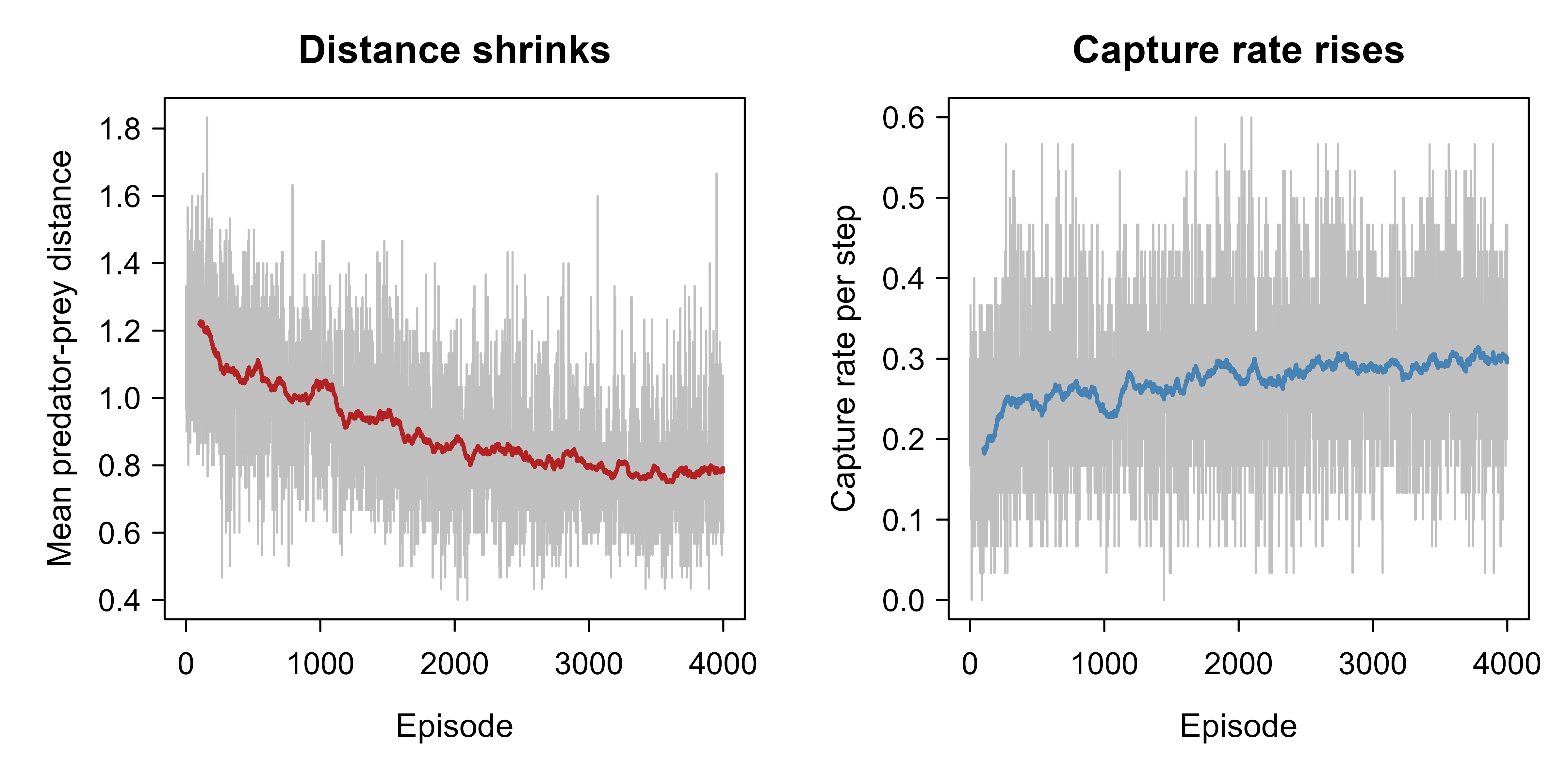
Finally, the learning curves. Plotting average distance and capture rate against episode shows the two diagnostics moving in opposite directions as the agents co-adapt: distance falls and capture rate rises, then both flatten, which is the visual signature of convergence to a stable joint policy. A moving average smooths the per-episode exploration noise. Both panels are drawn in one figure so they share a single label.
Show code
library(ggplot2)ma<-function(x, k=100L){as.numeric(stats::filter(x, rep(1/k, k), sides =1))}episode<-seq_len(n_episodes)op<-par(mfrow =c(1, 2), mar =c(4.2, 4.2, 2.5, 1))plot(episode, avg_dist_ep, type ="l", col ="grey75", xlab ="Episode", ylab ="Mean predator-prey distance", main ="Distance shrinks")lines(episode, ma(avg_dist_ep), col ="firebrick", lwd =2)plot(episode, capture_rate_ep, type ="l", col ="grey75", xlab ="Episode", ylab ="Capture rate per step", main ="Capture rate rises")lines(episode, ma(capture_rate_ep), col ="steelblue", lwd =2)par(op)
Figure 70.1: Joint behavior of two independent Q-learners in the five-cell pursuit game. Left: mean predator-prey ring distance per episode falls as the predator learns to close in. Right: capture rate per episode rises and stabilizes. The opposite-moving, then flattening, curves are the signature of convergence to a stable joint policy despite each agent learning against a non-stationary opponent.
Figure 70.1 shows the two diagnostics over training. The predator-prey distance (left) starts near the random-pair average and declines to a small floor, while the capture rate (right) climbs from near zero and stabilizes. The two curves move in opposite directions and then flatten together, which is what convergence to a stable joint policy looks like for this competitive game.
70.8 Practical guidance and pitfalls
The first decision is whether the problem is genuinely multi-agent at all. If the other “agents” are fixed (a scripted opponent, a static environment), you have a single-agent problem in disguise and should use single-agent RL, which is simpler and better understood. MARL earns its complexity only when several decision makers are learning or adapting at the same time.
Once you are in the multi-agent setting, start with the simplest baseline that could work: independent learners. They are easy to implement, scale to many agents, and frequently solve cooperative tasks well enough to set a bar. Treat them as a baseline, not a final answer, and watch for the symptoms of non-stationarity: returns that oscillate instead of settling, agents that keep cycling through strategies, or performance that depends heavily on the random seed.
When independent learning is unstable, reach for the structure that fits your deployment. If you control a simulator at training time but agents act locally at deployment, CTDE with a centralized critic is the standard fix, and in the fully cooperative case value decomposition (VDN, QMIX) gives decentralized execution almost for free. If the problem is two-player zero-sum, self-play with a population of past opponents is the proven recipe; never train against only the current self, or you will overfit to its quirks.
Several pitfalls recur often enough to name explicitly.
Stale replay in deep MARL. A replay buffer mixes transitions generated by opponents’ old policies, so the targets are obsolete. Use smaller buffers, importance weighting, or on-policy methods, and prefer centralized critics that condition on the joint action.
Equilibrium selection. General-sum games have many equilibria, and good group outcomes can be unstable. Do not assume convergence implies a good outcome; measure the actual joint return, and consider mechanisms (shared signals, reward shaping, communication) that steer toward the equilibrium you want.
Credit assignment in teams. With one shared reward, a single agent cannot tell whether its own action helped. Value decomposition and counterfactual baselines exist precisely to attribute the team reward back to individuals.
Self-play cycling and overfitting. Guard against rock-paper-scissors rotation and self-overfitting with opponent populations and league play, and evaluate against held-out opponents, not just the training pool.
Evaluation is harder than in single-agent RL. There is no fixed environment to score against; performance is relative to opponents. Report results against a panel of opponents (random, scripted, past selves, other algorithms), not a single matchup.
When to use this
Reach for MARL when several agents learn or adapt in a shared environment and their interactions are the point. Use the cooperative tools (VDN, QMIX, CTDE) for teams with a common goal, self-play with populations for two-player zero-sum competition, and treat mixed-motive problems with the most caution, because equilibrium selection and incentive conflicts make both training and evaluation delicate.
70.9 Reference: deep multi-agent learning sketch
The runnable demo is tabular because tables expose every moving part. Real systems with large or continuous state spaces replace each table with a network, and the CTDE structure becomes a centralized critic feeding decentralized actors. The sketch below shows the shape of a centralized critic plus per-agent actors in the style of MADDPG, an actor-critic method (Chapter 67) scaled up with the deep reinforcement learning machinery of Chapter 71. It is kept eval=FALSE because a full agent also needs an environment loop and replay buffer, and the deep-learning backend (Chapter 92) is not assumed available in this build.
Show code
library(torch)# Per-agent actor: maps a local observation to that agent's action logits.make_actor<-function(obs_dim, n_actions){nn_sequential(nn_linear(obs_dim, 64), nn_relu(),nn_linear(64, 64), nn_relu(),nn_linear(64, n_actions)# decentralized: sees only own obs)}# Centralized critic: conditions on the GLOBAL state and the JOINT action,# which is what removes non-stationarity during training.make_central_critic<-function(state_dim, joint_action_dim){nn_sequential(nn_linear(state_dim+joint_action_dim, 128), nn_relu(),nn_linear(128, 128), nn_relu(),nn_linear(128, 1)# scalar Q(s, a^1, ..., a^n))}n_agents<-3Lobs_dim<-8Ln_actions<-5Lstate_dim<-20Lactors<-lapply(seq_len(n_agents), function(i)make_actor(obs_dim, n_actions))critics<-lapply(seq_len(n_agents),function(i)make_central_critic(state_dim,n_agents*n_actions))# Training loop (omitted) for each agent i:# 1. critic target: y = r^i + gamma * Q_i^-(s', a'^1, ..., a'^n)# where a'^j come from the target actors (joint next action).# 2. critic loss: ( Q_i(s, a^1, ..., a^n) - y )^2# 3. actor update: ascend Q_i(s, ..., a^i = actor_i(o^i), ...)# 4. soft-update the target networks.# Execution uses ONLY actors[[i]](o^i): decentralized, no critic, no comms.
70.10 Further reading
The standard reference for reinforcement learning, including a chapter on the multi-agent extension, is Sutton and Barto (2018), Reinforcement Learning: An Introduction (2nd edition). For the multi-agent area specifically, the textbook by Albrecht, Christianos, and Schafer (2024), Multi-Agent Reinforcement Learning: Foundations and Modern Approaches, gives a current and thorough treatment, and the survey by Busoniu, Babuska, and De Schutter (2008) remains a clear map of the classical landscape.
The foundational game theory is Nash (1950) for the existence of equilibrium, von Neumann (1928) for the minimax theorem, and Aumann (1974) for correlated equilibrium. The stochastic-game formalism traces to Shapley (1953). For learning algorithms, Littman (1994) introduced minimax-Q for zero-sum stochastic games, Tan (1993) studied independent versus cooperative learners, Lowe et al. (2017) introduced MADDPG, Sunehag et al. (2018) value decomposition networks, and Rashid et al. (2018) QMIX. For self-play in practice, see Tesauro (1995) on TD-Gammon and Silver et al. (2016, 2018) on the AlphaGo and AlphaZero systems.
The same lens applies inside modern AI systems: a debate between two language models, a population of trading bots, or a fleet of delivery drones coordinating routes are all multi-agent systems whether or not they are described that way. Recognizing the structure tells you which tools, and which failure modes, to expect.↩︎
Source Code
# Multi-Agent Reinforcement Learning {#sec-multi-agent-rl}```{r}#| include: falsesource("_common.R")```A single reinforcement learning agent (@sec-rl-foundations) treats the world as a fixed, if uncertain, machine: it acts, the environment responds with a reward and a new state, and the rules behind that response never change. Now put two such agents in the same world and let each one learn. The "environment" that any one agent sees now contains the other agent, whose behavior is shifting from one episode to the next as it learns too. The ground the first agent is standing on is moving, because part of that ground is another mind. Multi-agent reinforcement learning (MARL) is the study of what happens, and what can be made to happen, when several learning agents share one environment.This shift sounds small but it breaks the foundation that single-agent theory rests on. The Markov decision process assumes stationary dynamics: the probability of the next state given the current state and action does not change over time. With other learners present, that assumption fails from the point of view of each individual agent, and most of the difficulty (and most of the interesting structure) in MARL flows from that one fact. The payoff for confronting it is large. Traffic routing, electricity markets, automated bidding, warehouse robots, network packet routing, and the self-play training behind game-playing systems are all genuinely multi-agent. Treating them as single-agent problems throws away the very interaction that defines them.^[The same lens applies inside modern AI systems: a debate between two language models, a population of trading bots, or a fleet of delivery drones coordinating routes are all multi-agent systems whether or not they are described that way. Recognizing the structure tells you which tools, and which failure modes, to expect.]::: {.callout-tip title="Intuition"}Single-agent RL is one player against nature, where nature does not adapt. MARL is several players against nature and against each other, where the other players learn and adapt. The reward you get for an action depends not only on what you do but on what everyone else decides to do at the same time.:::This chapter builds the ideas in order. It starts with the formal object that generalizes the MDP to many agents (the stochastic, or Markov, game), then separates the three regimes that change everything about how you should think (cooperative, competitive, and mixed). It introduces the equilibrium concepts that replace "the optimal policy" once there is more than one decision maker, explains why naive independent learning becomes unstable and what to do about it, and covers the dominant practical recipe (centralized training with decentralized execution) and the engine behind much recent progress (self-play). A fully runnable base-R demonstration trains two independent Q-learners in a small pursuit game and shows their joint behavior settling into a stable pattern, with a figure and a table. Deep MARL code is included as a reference but left unevaluated.## From one agent to many: the stochastic gameThe single-agent MDP is a tuple $(\mathcal{S}, \mathcal{A}, P, R, \gamma)$. The natural generalization to $n$ agents is the stochastic game (also called a Markov game), a tuple$$(\mathcal{S}, \{\mathcal{A}^i\}_{i=1}^{n}, P, \{R^i\}_{i=1}^{n}, \gamma).$$Here $\mathcal{S}$ is the shared set of states, and each agent $i$ has its own action set $\mathcal{A}^i$. At each step every agent picks an action simultaneously, forming the joint action $\mathbf{a} = (a^1, \dots, a^n)$ with $a^i \in \mathcal{A}^i$. The transition $P(s' \mid s, \mathbf{a})$ depends on the joint action, not on any single agent's action alone, and each agent receives its own reward $R^i(s, \mathbf{a})$. The discount $\gamma \in [0,1)$ plays the same role as before.The decisive change is that the reward and the transition depend on the joint action $\mathbf{a}$. From agent $i$'s seat, write the joint action as $(a^i, \mathbf{a}^{-i})$, separating its own action $a^i$ from the actions $\mathbf{a}^{-i}$ of everyone else. Agent $i$ controls only $a^i$; the term $\mathbf{a}^{-i}$ is chosen by the other agents according to policies that agent $i$ does not control and may not even observe.::: {.callout-important title="Key idea"}A single-agent MDP recovers the optimal policy because the dynamics are fixed. In a stochastic game the effective dynamics that agent $i$ experiences depend on $\mathbf{a}^{-i}$, which changes as the other agents learn. There is no single "best policy" in isolation; the best response for one agent is defined only relative to what the others are doing.:::Each agent follows a policy $\pi^i(a^i \mid s)$, and together they form a joint policy $\boldsymbol{\pi} = (\pi^1, \dots, \pi^n)$. Agent $i$ wants to maximize its own expected discounted return$$J^i(\boldsymbol{\pi}) = \mathbb{E}_{\boldsymbol{\pi}}\!\left[\sum_{t \ge 0} \gamma^t\, R^i(s_t, \mathbf{a}_t)\right],$$where the expectation is taken over the trajectory generated by the joint policy. The notation $J^i(\boldsymbol{\pi})$ makes the central tension explicit: agent $i$'s return is a function of every agent's policy, not just its own.::: {.callout-note}When $n = 1$, the stochastic game is exactly an MDP. When the state set $\mathcal{S}$ has a single element (the world never changes state), the stochastic game collapses to a repeated **matrix game**, the object studied in classical game theory. Stochastic games sit in between and above both: they are games with state and dynamics.:::### Value functions and Bellman equations for a fixed joint policyTo make the optimization in $J^i(\boldsymbol{\pi})$ precise, fix a joint policy $\boldsymbol{\pi} = (\pi^1, \dots, \pi^n)$ and define agent $i$'s state-value and action-value functions exactly as in the single-agent case, but evaluated along the trajectory the joint policy generates,$$V^i_{\boldsymbol{\pi}}(s) = \mathbb{E}_{\boldsymbol{\pi}}\!\left[\sum_{t \ge 0} \gamma^t R^i(s_t, \mathbf{a}_t) \,\Big|\, s_0 = s\right],\qquadQ^i_{\boldsymbol{\pi}}(s, \mathbf{a}) = \mathbb{E}_{\boldsymbol{\pi}}\!\left[\sum_{t \ge 0} \gamma^t R^i(s_t, \mathbf{a}_t) \,\Big|\, s_0 = s,\, \mathbf{a}_0 = \mathbf{a}\right].$$ {#eq-multi-agent-rl-value-defs}The crucial bookkeeping is that $Q^i_{\boldsymbol{\pi}}$ is indexed by the full joint action $\mathbf{a}$, because the one-step reward and the transition both depend on what every agent does. Because all other agents draw their actions from $\boldsymbol{\pi}^{-i}$ and the dynamics are Markov given the joint action, the same telescoping argument as in @sec-rl-foundations gives the policy-evaluation Bellman equation$$V^i_{\boldsymbol{\pi}}(s)= \sum_{\mathbf{a}} \Big(\textstyle\prod_{j} \pi^j(a^j \mid s)\Big)\Big[ R^i(s, \mathbf{a}) + \gamma \sum_{s'} P(s' \mid s, \mathbf{a})\, V^i_{\boldsymbol{\pi}}(s') \Big].$$ {#eq-multi-agent-rl-mg-bellman}Equation @eq-multi-agent-rl-mg-bellman is the foundation for everything that follows. For a fixed opponent profile $\boldsymbol{\pi}^{-i}$, define the induced single-agent transition and reward by marginalizing out the others,$$\tilde{P}^i(s' \mid s, a^i) = \sum_{\mathbf{a}^{-i}} \Big(\textstyle\prod_{j \ne i} \pi^j(a^j \mid s)\Big) P(s' \mid s, a^i, \mathbf{a}^{-i}),\qquad\tilde{R}^i(s, a^i) = \sum_{\mathbf{a}^{-i}} \Big(\textstyle\prod_{j \ne i} \pi^j(a^j \mid s)\Big) R^i(s, a^i, \mathbf{a}^{-i}).$$ {#eq-multi-agent-rl-induced-mdp}This is the formal version of the intuition that "the other agents are part of the environment": with $\boldsymbol{\pi}^{-i}$ held fixed, agent $i$ faces an ordinary MDP $(\mathcal{S}, \mathcal{A}^i, \tilde{P}^i, \tilde{R}^i, \gamma)$, and its best response is the optimal policy of that MDP. Two facts follow immediately. First, agent $i$'s best-response problem is well posed and solvable by single-agent methods whenever $\boldsymbol{\pi}^{-i}$ is stationary. Second, the non-stationarity pathology of @sec-multi-agent-rl is precisely the statement that $\tilde{P}^i$ and $\tilde{R}^i$ in @eq-multi-agent-rl-induced-mdp drift over training because $\boldsymbol{\pi}^{-i}$ is itself being updated, so the MDP agent $i$ is fitting is a moving target.### The matrix-game special caseA one-state stochastic game with two agents is a matrix game: each agent picks an action, and a payoff matrix maps the joint action to each agent's reward. These small games are the cleanest place to see the core phenomena, so it is worth fixing notation. With agent 1 choosing rows and agent 2 choosing columns, the reward to agent $i$ for joint action $(a^1, a^2)$ is an entry $R^i(a^1, a^2)$. The famous examples differ only in how those entries are arranged, and that arrangement is exactly what separates cooperation from competition.## Three regimes: cooperative, competitive, and mixedHow the rewards $\{R^i\}$ relate to each other determines almost everything about the problem. Three regimes are worth naming.In the fully cooperative regime, all agents share one reward: $R^1 = R^2 = \cdots = R^n = R$. Everyone wins or loses together, so the goal is joint coordination on behavior that maximizes the common return. A team of warehouse robots fulfilling orders, or sensors that jointly cover an area, fit here. The challenge is not conflict but coordination: agents must agree on who does what without necessarily talking.In the fully competitive regime, with two agents the rewards are exactly opposed: $R^1 = -R^2$. This is a zero-sum game. One agent's gain is the other's loss, as in chess, Go, or poker. Here the relevant solution concept is the minimax value, and self-play is especially powerful.In the mixed (general-sum) regime, rewards are neither identical nor opposite. Agents have partly aligned and partly conflicting interests. Most real systems live here: traffic, markets, and negotiation all combine shared interest (avoid gridlock, keep the market functioning) with private interest (get there first, maximize my profit). The prisoner's dilemma is the canonical small example, where each agent is individually tempted to defect even though mutual cooperation pays both more.::: {.callout-tip title="Intuition"}Cooperative means "we sink or swim together," competitive means "what helps me hurts you by the same amount," and mixed means "we are partly on the same team and partly rivals." The mixed case is the hardest because there is no single quantity everyone agrees to optimize, and outcomes that are good for the group can be unstable because some individual is tempted to deviate.:::@tbl-multi-agent-rl-regimes lays out the three regimes side by side, with the solution concept each one points to and a representative example.```{r tbl-multi-agent-rl-regimes}library(knitr)regimes <-data.frame(Regime =c("Cooperative", "Competitive (2-player)", "Mixed (general-sum)"),`Reward relation`=c("Shared: $R^1=\\dots=R^n$","Opposed: $R^1=-R^2$ (zero-sum)","Neither shared nor opposed"),`Core challenge`=c("Coordination", "Outplaying the opponent","Aligning conflicting incentives"),`Solution concept`=c("Team-optimal joint policy", "Minimax value","Nash / correlated equilibrium"),Example =c("Warehouse robot team", "Chess, Go, poker","Traffic, markets, prisoner's dilemma"),check.names =FALSE)kable(regimes,caption ="The three multi-agent regimes, distinguished by how the agents' rewards relate, the challenge each one poses, the solution concept it points to, and a representative example.")```## Equilibria: what replaces "the optimal policy"In a single-agent MDP the optimal policy is the one whose value dominates all others at every state. With several self-interested agents that definition is empty, because the value of agent $i$'s policy depends on the other agents' policies. The replacement comes from game theory.A joint policy $\boldsymbol{\pi}^* = (\pi^{1*}, \dots, \pi^{n*})$ is a Nash equilibrium if no single agent can improve its own expected return by unilaterally changing its policy while the others hold theirs fixed. Formally, for every agent $i$ and every alternative policy $\pi^i$,$$J^i(\pi^{i*}, \boldsymbol{\pi}^{-i*}) \;\ge\; J^i(\pi^{i}, \boldsymbol{\pi}^{-i*}).$$The condition says: given what everyone else is doing, agent $i$ is already playing a best response, so it has no incentive to move. A Nash equilibrium is a joint policy in which everyone is simultaneously best-responding to everyone else. It is a fixed point of the mutual best-response map.::: {.callout-important title="Key idea"}Nash equilibrium is a stability concept, not an optimality concept. It tells you where learning can stop changing, because nobody can do better alone. It does not promise the outcome is good for the group. The prisoner's dilemma has a unique Nash equilibrium (both defect) that is worse for both agents than mutual cooperation, which is not an equilibrium at all because each agent is tempted to deviate.:::Several facts about Nash equilibria shape practical MARL. Every finite game has at least one Nash equilibrium, possibly in mixed strategies (randomized policies), a result due to Nash (1950). But equilibria are not unique in general: a game can have many, and different learning algorithms, or different random seeds, can converge to different ones. In purely cooperative games the best outcome is an equilibrium, but so are bad coordination failures, so reaching the good equilibrium is itself the problem.For two-player zero-sum games there is a stronger and cleaner result. The minimax theorem (von Neumann, 1928) says each player has a security value: the best guaranteed payoff against a worst-case opponent. The value$$v = \max_{\pi^1} \min_{\pi^2} \; \mathbb{E}\big[R^1 \mid \pi^1, \pi^2\big] = \min_{\pi^2} \max_{\pi^1} \; \mathbb{E}\big[R^1 \mid \pi^1, \pi^2\big]$$is well defined: the order of "maximize then minimize" and "minimize then maximize" gives the same number. This is why competitive games are, in a precise sense, easier than mixed ones: there is a single value to converge to, and the optimal play does not depend on which of several equilibria the opponent prefers.#### Deriving the minimax value as a linear programThe minimax value is not just an existence statement; for a finite matrix game it is the solution of a linear program, which is both how it is computed in practice and why a unique value exists. Let agent 1 have action set $\{1, \dots, m\}$ and agent 2 have $\{1, \dots, k\}$, with payoff matrix $A \in \mathbb{R}^{m \times k}$ where $A_{j\ell} = R^1(j, \ell) = -R^2(j, \ell)$. A mixed strategy for agent 1 is a probability vector $x \in \Delta_m$ over its rows. If agent 1 commits to $x$, its worst-case expected payoff is attained at a pure best response by the opponent, because the opponent's payoff is linear in its own mixed strategy and a linear function on a simplex is minimized at a vertex,$$\min_{y \in \Delta_k} x^\top A y = \min_{\ell \in \{1, \dots, k\}} (x^\top A)_\ell = \min_{\ell} \sum_{j} x_j A_{j\ell}.$$ {#eq-multi-agent-rl-pure-response}Agent 1 therefore chooses $x$ to maximize this guaranteed floor. Introducing a scalar $v$ that lower-bounds the floor turns the inner minimum into a set of linear constraints,$$\max_{x \in \Delta_m,\, v}\; v\quad \text{subject to} \quad\sum_{j} x_j A_{j\ell} \ge v \;\; \text{for every column } \ell,\quad \sum_j x_j = 1, \quad x \ge 0.$$ {#eq-multi-agent-rl-minimax-lp}This is a linear program in $(x, v)$. Its dual, obtained by attaching multipliers $y_\ell \ge 0$ to the column constraints, is exactly the minimizing player's program: minimize $w$ subject to $\sum_\ell A_{j\ell} y_\ell \le w$ for every row $j$, with $y \in \Delta_k$. Linear-programming strong duality forces the two optimal values to coincide, $v^\star = w^\star$, and that common number is the game value $v$ in @eq-multi-agent-rl-minimax-lp-value below. The equality of the primal and dual optima is the minimax theorem; von Neumann's original proof predates LP duality, but the LP route is the constructive one used inside algorithms such as minimax-Q.$$v = \max_{x \in \Delta_m} \min_{\ell} \sum_j x_j A_{j\ell}.$$ {#eq-multi-agent-rl-minimax-lp-value}#### Minimax-Q and its contractionCarrying this into a stochastic game gives Littman's (1994) minimax-Q for the two-player zero-sum case. The state-action value $Q(s, a^1, a^2)$ now satisfies a Bellman equation in which the one-step continuation value at $s'$ is not a max (one decision maker) but the matrix-game value of the local payoff matrix $A_{s'} = [\,Q(s', \cdot, \cdot)\,]$,$$Q(s, a^1, a^2) = R^1(s, a^1, a^2) + \gamma \sum_{s'} P(s' \mid s, a^1, a^2)\, \mathrm{val}\big(Q(s', \cdot, \cdot)\big),$$ {#eq-multi-agent-rl-minimax-q}where $\mathrm{val}(M) = \max_{x \in \Delta} \min_{y \in \Delta} x^\top M y$ is computed by the LP @eq-multi-agent-rl-minimax-lp. The corresponding sample update replaces single-agent bootstrapping with the value operator,$$Q(s, a^1, a^2) \leftarrow (1 - \alpha) Q(s, a^1, a^2) + \alpha \big[\, r + \gamma\, \mathrm{val}\big(Q(s', \cdot, \cdot)\big)\,\big].$$ {#eq-multi-agent-rl-minimax-q-update}The reason this converges, unlike independent learning, is that the operator $\mathcal{T}$ defined by the right-hand side of @eq-multi-agent-rl-minimax-q is a $\gamma$-contraction in the supremum norm. The key lemma is that the matrix-game value is non-expansive: for any two matrices $M, M'$ of the same shape,$$\big|\, \mathrm{val}(M) - \mathrm{val}(M')\,\big| \le \max_{a^1, a^2} \big| M_{a^1 a^2} - M'_{a^1 a^2} \big|.$$ {#eq-multi-agent-rl-val-nonexpansive}To see @eq-multi-agent-rl-val-nonexpansive, let $x^\star$ achieve $\mathrm{val}(M)$. Then $\mathrm{val}(M') = \max_x \min_y x^\top M' y \ge \min_y (x^\star)^\top M' y \ge \min_y (x^\star)^\top M y - \|M - M'\|_\infty = \mathrm{val}(M) - \|M - M'\|_\infty$, where $\|\cdot\|_\infty$ is the entrywise sup norm; swapping the roles of $M$ and $M'$ gives the reverse inequality. Combining @eq-multi-agent-rl-val-nonexpansive with the discounted transition gives, for any two value tables $Q, Q'$,$$\|\mathcal{T} Q - \mathcal{T} Q'\|_\infty \le \gamma \max_{s'} \big|\mathrm{val}(Q(s', \cdot, \cdot)) - \mathrm{val}(Q'(s', \cdot, \cdot))\big| \le \gamma \|Q - Q'\|_\infty.$$ {#eq-multi-agent-rl-minimax-contraction}By the Banach fixed-point theorem $\mathcal{T}$ has a unique fixed point, and minimax-Q converges to it under the usual stochastic-approximation step-size conditions $\sum_t \alpha_t = \infty$, $\sum_t \alpha_t^2 < \infty$. This is the formal payoff of zero-sum structure: a single contraction with a single fixed point, exactly mirroring single-agent Q-learning, which independent learners in general-sum games do not enjoy.The non-expansiveness lemma @eq-multi-agent-rl-val-nonexpansive is the linchpin of that argument, so it is worth confirming numerically. The following base-R check evaluates the matrix-game value on a fine grid of the row player's mixed strategies (a $2 \times 2$ game makes the simplex one-dimensional) and verifies that perturbing the payoff matrix changes the value by no more than the largest entrywise perturbation.```{r multi-agent-rl-val-nonexpansive}set.seed(1)# val(M) for a 2-action row player: max over a grid of mixed strategies x# of the worst-case column payoff min_l (x^T M)_l.val2 <-function(M, grid =2000L) { xs <-seq(0, 1, length.out = grid) best <--Inffor (x in xs) { p <-c(x, 1- x) # row mixed strategy col_payoffs <-as.numeric(p %*% M) # one entry per column floor_x <-min(col_payoffs)if (floor_x > best) best <- floor_x } best}# Verify |val(M) - val(M')| <= ||M - M'||_inf over random perturbations.max_ratio <-0for (rep in1:500) { M <-matrix(rnorm(4), 2, 2) E <-matrix(rnorm(4, sd =0.3), 2, 2) Mp <- M + E lhs <-abs(val2(M) -val2(Mp)) rhs <-max(abs(E)) # entrywise sup norm of the perturbation max_ratio <-max(max_ratio, lhs / rhs)}cat("Largest observed |val(M)-val(M')| / ||M-M'||_inf:",round(max_ratio, 4), "\n")cat("Non-expansiveness (ratio <= 1) holds:", max_ratio <=1+1e-3, "\n")```The ratio never exceeds one (up to the grid resolution), confirming that the value operator is non-expansive and hence that $\mathcal{T}$ in @eq-multi-agent-rl-minimax-contraction contracts at rate $\gamma$.::: {.callout-note}A **correlated equilibrium** (Aumann, 1974) generalizes Nash by allowing the agents' randomized choices to be coordinated by a shared signal (think of a traffic light coordinating who goes). It can achieve outcomes no independent Nash equilibrium reaches, and it is often easier to compute, which makes it relevant when a central coordinator is available at execution time.:::The computational gap between the two solution concepts is real and shapes algorithm design. Computing a minimax (zero-sum) equilibrium is a linear program, polynomial in the number of actions, as @eq-multi-agent-rl-minimax-lp shows. Computing a Nash equilibrium of a general-sum game is PPAD-complete (Daskalakis, Goldberg, and Papadimitriou, 2009), believed intractable in the worst case even for two players, so there is no known efficient algorithm and no learning dynamics guaranteed to converge to one in general. A correlated equilibrium, by contrast, is the solution of a single linear program over the joint-action distribution and is computable in polynomial time. This hardness is the deep reason MARL theory is clean for zero-sum games and murky for general-sum ones, and it justifies the practical retreat to "measure the realized joint return" rather than "certify an equilibrium."### Learning dynamics and convergenceEquilibrium is a fixed point of the mutual best-response map, but it does not say whether any learning process reaches it. The classical positive result is fictitious play (Brown, 1951): each agent best-responds to the empirical frequency of its opponents' past actions. Writing $\bar{x}^{-i}_t$ for the running average of the others' play, agent $i$ plays a best response $\mathrm{BR}^i(\bar{x}^{-i}_t)$ and the averages update as $\bar{x}^i_{t+1} = (1 - \tfrac{1}{t+1})\bar{x}^i_t + \tfrac{1}{t+1} e_{a^i_t}$. Fictitious play's empirical frequencies converge to a Nash equilibrium in two-player zero-sum games (Robinson, 1951) and in potential games, but they can cycle indefinitely in general-sum games (Shapley's famous $3 \times 3$ counterexample). Independent Q-learning is a stochastic, value-based cousin of these dynamics, which is why it inherits both their occasional success and their lack of a general guarantee. Modern convergent algorithms for the zero-sum case, such as optimistic gradient and regret-matching variants, achieve last-iterate or time-average convergence by adding a correction that counteracts the rotational component of the best-response dynamics that causes the cycling.## Independent learners and the non-stationarity problemThe simplest thing to try in a multi-agent setting is to ignore the multi-agent structure entirely: give each agent its own single-agent algorithm, let it treat the other agents as part of the environment, and let them all learn at once. This is independent learning, and the version using Q-learning is Independent Q-Learning (IQL), going back to Tan (1993). Each agent $i$ keeps its own table $Q^i(s, a^i)$, indexed by its own action only, and applies the ordinary Q-learning update$$Q^i(s, a^i) \leftarrow Q^i(s, a^i) + \alpha\Big[\, r^i + \gamma \max_{b \in \mathcal{A}^i} Q^i(s', b) - Q^i(s, a^i)\,\Big],$$ {#eq-multi-agent-rl-iql-update}pretending it lives in an MDP. Comparing @eq-multi-agent-rl-iql-update with the minimax-Q update @eq-multi-agent-rl-minimax-q-update isolates the problem exactly: IQL maxes over its own action alone, treating the opponent's contribution as fixed environment noise, whereas minimax-Q applies the game-value operator to the joint table. The target in @eq-multi-agent-rl-iql-update is an estimate of the optimal value of the induced MDP $(\mathcal{S}, \mathcal{A}^i, \tilde{P}^i, \tilde{R}^i, \gamma)$ from @eq-multi-agent-rl-induced-mdp. Because $\tilde{P}^i$ and $\tilde{R}^i$ change every time another agent updates, the operator that IQL is implicitly iterating is itself changing between updates, so the contraction argument @eq-multi-agent-rl-minimax-contraction does not apply and the Banach fixed point may not exist. That is the precise sense in which IQL has no convergence guarantee.The appeal is obvious: it is trivial to implement, it scales to many agents because each one is small, and at execution time each agent acts on its own observation with no communication. The drawback is equally fundamental. From agent $i$'s perspective the transition and reward depend on $\mathbf{a}^{-i}$, which is generated by the other agents' policies, and those policies change as the other agents learn. The dynamics agent $i$ is trying to fit are non-stationary: the very thing being estimated keeps shifting.::: {.callout-warning}Non-stationarity from concurrent learning is the central pitfall of MARL. The convergence guarantees of single-agent Q-learning assume a stationary environment, and that assumption is violated by construction when other agents learn. Independent learners can oscillate, chase each other, or settle on a poor joint policy. The experience replay buffer that stabilizes single-agent DQN makes this worse, because old transitions were generated by the other agents' old (now obsolete) policies, so the replayed targets are stale.:::There is a useful tension here. If you give agent $i$ a perfect model of the other agents' current policies, its problem becomes a stationary MDP again and ordinary RL applies, but that model is exactly what is changing. Practical approaches manage the non-stationarity rather than eliminate it. Slowing down learning (small learning rates) and using decaying exploration so the agents stop perturbing each other late in training both help. Letting agents observe or estimate the others' actions during training (the next two sections) helps more. In practice independent learning often works surprisingly well as a baseline, especially in cooperative tasks, which is why it remains a standard first thing to try despite having no general guarantees.## Centralized training with decentralized executionThe most influential practical idea in modern MARL resolves the non-stationarity tension by separating two phases. During training, you are usually building the system in a simulator or a controlled setting where you can see everything: every agent's observation, every agent's action, the global state. During execution, each deployed agent typically sees only its own local observation and must act without waiting on the others. The recipe known as centralized training with decentralized execution (CTDE) exploits exactly this asymmetry.The idea is to use the extra information available at training time to stabilize learning, while keeping the deployed policies decentralized so they can run independently. Concretely, each agent has its own policy $\pi^i(a^i \mid o^i)$ that conditions only on its local observation $o^i$, so it can be executed alone. But the critic that trains those policies is allowed to see the global state and the joint action. A centralized critic $Q(s, a^1, \dots, a^n)$ that conditions on everyone's actions is, from any single agent's view, stationary: it does not suffer the moving-target problem, because it already accounts for what the others did. The actors stay local; the critic is global. This is the structure behind algorithms such as MADDPG (Lowe et al., 2017) and the value-decomposition family discussed below.::: {.callout-important title="Key idea"}CTDE buys stability with information you only need temporarily. The centralized critic removes non-stationarity during learning because it conditions on the joint action; the decentralized actors keep deployment cheap and communication-free. You pay for the global view once, at training time, and never again.:::In the cooperative case there is an elegant specialization. When all agents share one reward, you can try to learn a single joint value $Q_{\text{tot}}(s, \mathbf{a})$ but represent it as a combination of per-agent values $Q^i(o^i, a^i)$ so that each agent can act greedily on its own piece. Value decomposition networks (Sunehag et al., 2018) use a simple sum, $Q_{\text{tot}} = \sum_i Q^i$, and QMIX (Rashid et al., 2018) uses a monotonic mixing function so that$$\frac{\partial Q_{\text{tot}}}{\partial Q^i} \ge 0 \quad \text{for every } i.$$The monotonicity condition is what matters: it guarantees that the action maximizing the global $Q_{\text{tot}}$ is obtained by each agent independently maximizing its own $Q^i$. That single inequality lets a team train against one shared reward while still executing in a fully decentralized way.The decentralization property has a one-line proof, and it is worth seeing because it explains why monotonicity, and not some weaker condition, is exactly what is required. Write $Q_{\text{tot}}(s, \mathbf{a}) = f_s(Q^1(o^1, a^1), \dots, Q^n(o^n, a^n))$ where $f_s$ is the mixing function and $\partial f_s / \partial Q^i \ge 0$ for every $i$. Decentralized greedy execution is correct when$$\arg\max_{\mathbf{a}} Q_{\text{tot}}(s, \mathbf{a}) = \Big( \arg\max_{a^1} Q^1(o^1, a^1),\, \dots,\, \arg\max_{a^n} Q^n(o^n, a^n) \Big),$$ {#eq-multi-agent-rl-igm}a property called individual-global-max (IGM). Suppose each agent picks its own greedy action $a^{i\star} = \arg\max_{a^i} Q^i(o^i, a^i)$. For any other joint action $\mathbf{a}$, change one coordinate at a time from $\mathbf{a}$ to $\mathbf{a}^\star$. At each single-coordinate step the corresponding $Q^i$ does not decrease, since $a^{i\star}$ maximizes it, and because $f_s$ is non-decreasing in that argument, $Q_{\text{tot}}$ does not decrease either. Chaining the $n$ steps gives $Q_{\text{tot}}(s, \mathbf{a}^\star) \ge Q_{\text{tot}}(s, \mathbf{a})$, so $\mathbf{a}^\star$ is a global maximizer and @eq-multi-agent-rl-igm holds. VDN's sum is the special case $f_s(\cdot) = \sum_i Q^i$, whose partials are all $1 > 0$. QMIX enforces $\partial f_s / \partial Q^i \ge 0$ by constraining the mixing network's weights to be non-negative (typically the absolute value of hypernetwork outputs), which buys a strictly richer, state-dependent class of mixers than the plain sum while preserving IGM.::: {.callout-warning}Monotonicity is sufficient for IGM but not necessary, and it caps representational power. Any task whose optimal joint value is non-monotone in the per-agent utilities, the classic example being a coordination game where the best joint action requires both agents to deviate together from their individually greedy choices, cannot be represented exactly by VDN or QMIX. This is the motivation for later factorizations (QTRAN, weighted QMIX, QPLEX) that enforce IGM without the monotonicity straitjacket.:::## Self-playIn two-player zero-sum games there is no fixed opponent to learn against, so where does training data come from? Self-play answers: let the agent play against copies of itself. The agent improves, the opponent (a copy) improves with it, and the difficulty of the opposition automatically tracks the agent's own skill. This produces a natural curriculum (@sec-curriculum-learning), easy when both sides are weak, progressively harder as both improve, without anyone hand-designing the stages.Self-play is the engine behind the strongest game-playing systems, from TD-Gammon (Tesauro, 1995) through the AlphaGo and AlphaZero line (Silver et al., 2016, 2018). Its theoretical comfort comes from the minimax structure: in a zero-sum game there is a single value to converge to, and an agent that becomes unbeatable by every version of itself is approaching minimax-optimal play.The right way to make "approaching optimal play" precise is exploitability. For a policy $\pi$ in a two-player zero-sum game, the exploitability is the gap between the game value $v$ and the worst-case return $\pi$ guarantees,$$\mathrm{expl}(\pi) = v - \min_{\pi'} \mathbb{E}\big[R^1 \mid \pi, \pi'\big] = \max_{\pi'} \mathbb{E}\big[R^1 \mid \pi', \pi\big] - v \ge 0,$$ {#eq-multi-agent-rl-exploitability}with equality to zero exactly when $\pi$ is a minimax (Nash) strategy. Exploitability is the principled evaluation metric for zero-sum self-play because it does not depend on which opponent you happened to train against; it measures performance against a best-responding adversary. The failure mode of naive self-play is now sharp. Training only against the current self drives down the return against that specific opponent, which is the second term evaluated at $\pi' = \pi_{\text{current}}$, not the worst-case minimum in @eq-multi-agent-rl-exploitability, so exploitability can stay high or even rise while self-match performance looks flat (the rock-paper-scissors cycle). Population and league methods approximate the inner $\min$ by a maximum over a diverse opponent set, which is why beating your whole history is a far better proxy for low exploitability than beating your current self. Fictitious self-play (Heinrich, Lanctot, and Silver, 2015) makes this exact: best-responding to the average of all past policies is the deep-RL analogue of fictitious play and inherits its convergence to the minimax value in zero-sum games.::: {.callout-warning}Self-play has characteristic failure modes. The agents can fall into a narrow rock-paper-scissors cycle where strategy A beats B, B beats C, and C beats A, so apparent progress is just rotation with no real improvement. They can also **overfit to themselves**, becoming strong against their own quirks but brittle against any outside opponent. The standard defenses are to keep a **population** of past versions and train against a mixture of them (so the agent must beat its whole history, not just its current self), and to add **league** structure with diverse opponent types. A frozen pool of past selves is the cheap version every practitioner reaches for first.:::## Runnable demo: two independent Q-learners in a pursuit gameThe clearest way to see joint behavior emerge is to watch two independent learners settle into a stable pattern in a small game implemented in nothing but base R. The setting is a tiny pursuit game on a one-dimensional ring of five cells. A predator and a prey each occupy a cell. At each step both move simultaneously (left, stay, or right) around the ring. The predator is rewarded for landing on the prey's cell and the prey is penalized for being caught, so this is a competitive (zero-sum-flavored) game with state: the state is the pair of positions, which makes it a genuine stochastic game rather than a one-shot matrix game.Each agent runs ordinary tabular Q-learning, treating the other agent as part of the environment. This is exactly the independent-learning setup from above, with all of its non-stationarity, and the point of the demo is to show that despite the lack of guarantees, the two agents' joint behavior converges to a stable, sensible pattern: the predator learns to close the gap and the prey learns to flee, so the distance between them collapses to its minimum and the capture rate climbs.::: {.callout-tip}Read the next chunks as one story. The first defines the ring environment and the joint transition. The second runs concurrent independent Q-learning for both agents. The third reports the learned greedy behavior as a table. The last two produce a single learning-curve figure. Everything is base R plus `ggplot2`, so you can inspect either `Q_pred` or `Q_prey` at any point.:::```{r multi-agent-rl-setup}.libPaths(c("C:/Users/miken/R/library-4.4", .libPaths()))set.seed(42)# Ring of N cells, positions 0..N-1. Two agents: predator and prey.N <-5Lmoves <-c(-1L, 0L, 1L) # left, stay, right (around the ring)move_names <-c("left", "stay", "right")n_actions <-length(moves)# Ring distance between two positions (0 .. floor(N/2)).ring_dist <-function(p, q) { d <-abs(p - q)min(d, N - d)}# Apply a move on the ring (wraps around).move_pos <-function(p, m) ((p + m) %% N)# The prey is a touch slower than the predator: its intended move only# succeeds with this probability, otherwise it slips and stays put. This# small speed edge is what lets pursuit actually succeed on a tiny ring# (with exactly equal speeds the prey could evade forever).prey_success <-0.7# State id from the pair of positions (0..N-1 each) -> 1..N^2.state_id <-function(p_pred, p_prey) p_pred * N + p_prey +1Ln_states <- N * N# Rewards for a transition that lands at (pred', prey').# Predator wants to be on the prey; prey wants to be away.reward_pred <-function(pred2, prey2) {if (pred2 == prey2) 1.0else-0.05# small step cost encourages closing in}reward_prey <-function(pred2, prey2) {if (pred2 == prey2) -1.0else0.05# rewarded for staying free}```With the environment fixed, both agents learn at the same time. Each keeps its own Q-table indexed by the shared state (the position pair) and its own action. The episode resets to random positions, and exploration decays so the agents perturb each other less as training proceeds.```{r multi-agent-rl-train}gamma <-0.9alpha <-0.2n_episodes <-4000Lmax_steps <-30Leps_start <-1.0eps_end <-0.05eps_decay <-0.999Q_pred <-matrix(0, nrow = n_states, ncol = n_actions)Q_prey <-matrix(0, nrow = n_states, ncol = n_actions)epsilon <- eps_start# Per-episode diagnostics.avg_dist_ep <-numeric(n_episodes) # mean predator-prey distancecapture_rate_ep <-numeric(n_episodes) # fraction of steps with a capturepick_action <-function(Qrow, eps) {if (runif(1) < eps) sample.int(n_actions, 1L) elsewhich.max(Qrow)}for (ep inseq_len(n_episodes)) {# Random start with the two agents apart. p_pred <-sample(0:(N -1L), 1L) p_prey <-sample(0:(N -1L), 1L)while (p_prey == p_pred) p_prey <-sample(0:(N -1L), 1L) dist_sum <-0 captures <-0for (t inseq_len(max_steps)) { s <-state_id(p_pred, p_prey) a_pred <-pick_action(Q_pred[s, ], epsilon) a_prey <-pick_action(Q_prey[s, ], epsilon)# Simultaneous joint transition (the prey may slip and stay put). pred2 <-move_pos(p_pred, moves[a_pred]) prey_move <-if (runif(1) < prey_success) moves[a_prey] else0L prey2 <-move_pos(p_prey, prey_move) s2 <-state_id(pred2, prey2) r_pred <-reward_pred(pred2, prey2) r_prey <-reward_prey(pred2, prey2)# Each agent applies its own independent Q-learning update. Q_pred[s, a_pred] <- Q_pred[s, a_pred] + alpha * (r_pred + gamma *max(Q_pred[s2, ]) - Q_pred[s, a_pred]) Q_prey[s, a_prey] <- Q_prey[s, a_prey] + alpha * (r_prey + gamma *max(Q_prey[s2, ]) - Q_prey[s, a_prey]) dist_sum <- dist_sum +ring_dist(pred2, prey2)if (pred2 == prey2) captures <- captures +1L p_pred <- pred2; p_prey <- prey2 } avg_dist_ep[ep] <- dist_sum / max_steps capture_rate_ep[ep] <- captures / max_steps epsilon <-max(eps_end, epsilon * eps_decay)}cat("Final epsilon:", round(epsilon, 3), "\n")cat("Mean distance, first 200 episodes:",round(mean(avg_dist_ep[1:200]), 3), "\n")cat("Mean distance, last 200 episodes: ",round(mean(avg_dist_ep[(n_episodes -199):n_episodes]), 3), "\n")```The printed summary already tells the story: the average predator-prey distance shrinks from its early random value to a small late value, meaning the predator has learned to hunt and the prey, while it tries to escape, cannot outrun a competent pursuer on so small a ring. To make the convergence concrete, the next chunk extracts the greedy policy of each agent in a fixed diagnostic state and reports it as a table.```{r tbl-multi-agent-rl-policy-table}library(knitr)# Inspect greedy actions across a few representative states where the# predator is fixed at cell 0 and the prey sits at each possible cell.diag_rows <-lapply(0:(N -1L), function(prey_pos) {if (prey_pos ==0L) return(NULL) # skip the already-caught state s <-state_id(0L, prey_pos)data.frame(`Prey cell`= prey_pos,`Ring gap`=ring_dist(0L, prey_pos),`Predator move`= move_names[which.max(Q_pred[s, ])],`Prey move`= move_names[which.max(Q_prey[s, ])],check.names =FALSE )})policy_tbl <-do.call(rbind, diag_rows)kable(policy_tbl,caption ="Learned greedy moves with the predator fixed at cell 0 and the prey at each other cell on the five-cell ring. The predator consistently steps toward the prey along the shorter arc, and the prey steps away, the signature of a stable pursuit-evasion pattern.")```@tbl-multi-agent-rl-policy-table shows the learned greedy moves: with the predator at cell 0, it steps along the shorter arc toward the prey while the prey steps the other way, which is exactly the best-response behavior a Nash equilibrium of this pursuit game should produce. Despite each agent learning independently against a moving target, the joint policy has settled into a coherent, stable pattern.Finally, the learning curves. Plotting average distance and capture rate against episode shows the two diagnostics moving in opposite directions as the agents co-adapt: distance falls and capture rate rises, then both flatten, which is the visual signature of convergence to a stable joint policy. A moving average smooths the per-episode exploration noise. Both panels are drawn in one figure so they share a single label.```{r fig-multi-agent-rl-learning-curve, fig.cap="Joint behavior of two independent Q-learners in the five-cell pursuit game. Left: mean predator-prey ring distance per episode falls as the predator learns to close in. Right: capture rate per episode rises and stabilizes. The opposite-moving, then flattening, curves are the signature of convergence to a stable joint policy despite each agent learning against a non-stationary opponent.", fig.width=8, fig.height=4}library(ggplot2)ma <-function(x, k =100L) {as.numeric(stats::filter(x, rep(1/ k, k), sides =1))}episode <-seq_len(n_episodes)op <-par(mfrow =c(1, 2), mar =c(4.2, 4.2, 2.5, 1))plot(episode, avg_dist_ep, type ="l", col ="grey75",xlab ="Episode", ylab ="Mean predator-prey distance",main ="Distance shrinks")lines(episode, ma(avg_dist_ep), col ="firebrick", lwd =2)plot(episode, capture_rate_ep, type ="l", col ="grey75",xlab ="Episode", ylab ="Capture rate per step",main ="Capture rate rises")lines(episode, ma(capture_rate_ep), col ="steelblue", lwd =2)par(op)```@fig-multi-agent-rl-learning-curve shows the two diagnostics over training. The predator-prey distance (left) starts near the random-pair average and declines to a small floor, while the capture rate (right) climbs from near zero and stabilizes. The two curves move in opposite directions and then flatten together, which is what convergence to a stable joint policy looks like for this competitive game.## Practical guidance and pitfallsThe first decision is whether the problem is genuinely multi-agent at all. If the other "agents" are fixed (a scripted opponent, a static environment), you have a single-agent problem in disguise and should use single-agent RL, which is simpler and better understood. MARL earns its complexity only when several decision makers are learning or adapting at the same time.Once you are in the multi-agent setting, start with the simplest baseline that could work: independent learners. They are easy to implement, scale to many agents, and frequently solve cooperative tasks well enough to set a bar. Treat them as a baseline, not a final answer, and watch for the symptoms of non-stationarity: returns that oscillate instead of settling, agents that keep cycling through strategies, or performance that depends heavily on the random seed.When independent learning is unstable, reach for the structure that fits your deployment. If you control a simulator at training time but agents act locally at deployment, CTDE with a centralized critic is the standard fix, and in the fully cooperative case value decomposition (VDN, QMIX) gives decentralized execution almost for free. If the problem is two-player zero-sum, self-play with a population of past opponents is the proven recipe; never train against only the current self, or you will overfit to its quirks.Several pitfalls recur often enough to name explicitly.- Stale replay in deep MARL. A replay buffer mixes transitions generated by opponents' old policies, so the targets are obsolete. Use smaller buffers, importance weighting, or on-policy methods, and prefer centralized critics that condition on the joint action.- Equilibrium selection. General-sum games have many equilibria, and good group outcomes can be unstable. Do not assume convergence implies a good outcome; measure the actual joint return, and consider mechanisms (shared signals, reward shaping, communication) that steer toward the equilibrium you want.- Credit assignment in teams. With one shared reward, a single agent cannot tell whether its own action helped. Value decomposition and counterfactual baselines exist precisely to attribute the team reward back to individuals.- Self-play cycling and overfitting. Guard against rock-paper-scissors rotation and self-overfitting with opponent populations and league play, and evaluate against held-out opponents, not just the training pool.- Evaluation is harder than in single-agent RL. There is no fixed environment to score against; performance is relative to opponents. Report results against a panel of opponents (random, scripted, past selves, other algorithms), not a single matchup.::: {.callout-tip title="When to use this"}Reach for MARL when several agents learn or adapt in a shared environment and their interactions are the point. Use the cooperative tools (VDN, QMIX, CTDE) for teams with a common goal, self-play with populations for two-player zero-sum competition, and treat mixed-motive problems with the most caution, because equilibrium selection and incentive conflicts make both training and evaluation delicate.:::## Reference: deep multi-agent learning sketchThe runnable demo is tabular because tables expose every moving part. Real systems with large or continuous state spaces replace each table with a network, and the CTDE structure becomes a centralized critic feeding decentralized actors. The sketch below shows the shape of a centralized critic plus per-agent actors in the style of MADDPG, an actor-critic method (@sec-policy-gradient) scaled up with the deep reinforcement learning machinery of @sec-deep-reinforcement-learning. It is kept `eval=FALSE` because a full agent also needs an environment loop and replay buffer, and the deep-learning backend (@sec-torch-for-r) is not assumed available in this build.```{r multi-agent-rl-maddpg-sketch, eval=FALSE}library(torch)# Per-agent actor: maps a local observation to that agent's action logits.make_actor <-function(obs_dim, n_actions) {nn_sequential(nn_linear(obs_dim, 64), nn_relu(),nn_linear(64, 64), nn_relu(),nn_linear(64, n_actions) # decentralized: sees only own obs )}# Centralized critic: conditions on the GLOBAL state and the JOINT action,# which is what removes non-stationarity during training.make_central_critic <-function(state_dim, joint_action_dim) {nn_sequential(nn_linear(state_dim + joint_action_dim, 128), nn_relu(),nn_linear(128, 128), nn_relu(),nn_linear(128, 1) # scalar Q(s, a^1, ..., a^n) )}n_agents <-3Lobs_dim <-8Ln_actions <-5Lstate_dim <-20Lactors <-lapply(seq_len(n_agents), function(i) make_actor(obs_dim, n_actions))critics <-lapply(seq_len(n_agents),function(i) make_central_critic(state_dim, n_agents * n_actions))# Training loop (omitted) for each agent i:# 1. critic target: y = r^i + gamma * Q_i^-(s', a'^1, ..., a'^n)# where a'^j come from the target actors (joint next action).# 2. critic loss: ( Q_i(s, a^1, ..., a^n) - y )^2# 3. actor update: ascend Q_i(s, ..., a^i = actor_i(o^i), ...)# 4. soft-update the target networks.# Execution uses ONLY actors[[i]](o^i): decentralized, no critic, no comms.```## Further readingThe standard reference for reinforcement learning, including a chapter on the multi-agent extension, is Sutton and Barto (2018), *Reinforcement Learning: An Introduction* (2nd edition). For the multi-agent area specifically, the textbook by Albrecht, Christianos, and Schafer (2024), *Multi-Agent Reinforcement Learning: Foundations and Modern Approaches*, gives a current and thorough treatment, and the survey by Busoniu, Babuska, and De Schutter (2008) remains a clear map of the classical landscape.The foundational game theory is Nash (1950) for the existence of equilibrium, von Neumann (1928) for the minimax theorem, and Aumann (1974) for correlated equilibrium. The stochastic-game formalism traces to Shapley (1953). For learning algorithms, Littman (1994) introduced minimax-Q for zero-sum stochastic games, Tan (1993) studied independent versus cooperative learners, Lowe et al. (2017) introduced MADDPG, Sunehag et al. (2018) value decomposition networks, and Rashid et al. (2018) QMIX. For self-play in practice, see Tesauro (1995) on TD-Gammon and Silver et al. (2016, 2018) on the AlphaGo and AlphaZero systems.