Imagine you are trying to predict house prices and your first model is a small, blunt decision tree (Chapter 8). It captures the broad pattern (bigger houses cost more) but it misses many details, and its errors are large for certain neighborhoods. A natural human reaction would be to look at where the model went wrong and build a second, focused model that specializes in fixing those mistakes, then a third that fixes what is still wrong, and so on. Boosting is exactly this idea made precise: it builds a sequence of simple models, each one trained to correct the errors left behind by the models before it.
This stands in contrast to bagging and random forests (Chapter 13), where many trees are grown independently on bootstrap samples and then averaged. Boosting grows trees sequentially: each new tree depends strongly on the trees already built, because it is fit to what they got wrong. There are no bootstrap samples in classic boosting; instead, we repeatedly fit small trees to the residuals (the leftover error), not to the original response \(Y\) directly.
The phrase you will hear in the literature is that boosting “learns slowly.” Rather than fitting one large tree that tries to capture everything at once (sometimes called “fitting the data hard”), boosting nudges the model in the right direction a little at a time, scaling each new tree by a small shrinkage factor \(\lambda\). Learning slowly turns out to be a feature, not a bug: it concentrates effort on the parts of the problem that are still poorly fit and it guards against overfitting.
In this chapter you will build up boosting from its conceptual core to its modern, production-grade implementations. We start with the intuition (gradient descent and slow learning), then give the precise algorithms for regression and classification, work through the original AdaBoost, generalize to gradient boosting, and finish with the libraries you will actually use in practice (gbm, xgboost, lightgbm, and h2o), along with the interpretation tools (variable importance, partial dependence, and LIME) that make a boosted model explainable.
Key idea
Boosting combines many “weak” learners (models that are only slightly better than guessing) into one strong “committee,” by training each new learner to fix the mistakes of the current ensemble.
A few facts worth keeping in mind from the start. Boosting was originally designed for classification (the classic algorithm is AdaBoost.M1 (Freund and Schapire 1997), and it is sometimes called hypothesis boosting), but it extends naturally to regression. It is widely regarded as one of the best off-the-shelf predictors available.1
When should you reach for boosting, and what are the tradeoffs? The following lists summarize the practical case.
Boosting tends to offer:
Good predictive accuracy, often state of the art on tabular data.
Several hyperparameters to tune, which gives you a lot of flexibility.
Little need for preprocessing.
Built-in handling of missing data in many implementations (no imputation needed).
The costs to weigh against those benefits are:
Because it relentlessly drives down training error, a gradient boosting machine (GBM) can overemphasize outliers and overfit. Cross-validation (Chapter 1) is the main defense.
It can be computationally expensive, especially during a large grid search over hyperparameters.
Underneath all of this, the general framework of boosting is a stagewise additive model built from \(B\) regression trees, which connects it directly to the additive models of Chapter 6:
\[
f(x) = \sum_{b=1}^B f^b (x)
\]
The rest of the chapter unpacks how those component functions \(f^b\) are chosen and combined.
11.1 Gradient Descent
Before the algorithms, it helps to name the engine that drives modern boosting: gradient descent. Gradient descent is a general recipe for minimizing a function by repeatedly taking a small step in the direction that decreases it fastest (the negative gradient). Gradient boosting is, quite literally, gradient descent applied in “function space,” where each step is a new tree.
The reasons this framing matters:
Gradient boosting can be generalized to minimize many different loss functions (for example mean squared error or mean absolute error), not just one.
The core idea is to tweak the model iteratively to minimize a cost function.
It works for any differentiable loss function, which is what lets us swap in losses suited to regression, classification, or ranking.
Intuition
If the loss is a hill you want to walk down, the gradient points uphill. Boosting reads off the (negative) gradient at the current model, fits a tree to it, and takes a small downhill step scaled by the learning rate.
If you would like a careful walk-through of the underlying optimization, you can refer to the first book for more detail.
11.2 Tuning
Boosting gives you several knobs, and getting good performance is largely a matter of setting them sensibly. Here are the main ones, with what each controls:
Number of trees: how many sequential trees to grow.
Depth of trees: how many splits \(d\) each tree is allowed (this controls how much interaction between variables a single tree can capture).
Learning rate (shrinkage): smaller values reduce overfitting but require more trees and longer fitting time.
Subsampling: training each tree on a random subset of the data adds randomness that can reduce overfitting; tune it with cross-validation (Chapter 1).
We will see these same parameters reappear under slightly different names in every library later in the chapter.
11.3 Regression Boosting
With the intuition in place, here is the precise algorithm for boosting regression trees. Read it as “start from nothing, then repeatedly fit a small tree to the current residuals and add a shrunken version of it back in.”
Set \(\hat{f}(x) = 0\) and \(r_i = y_i \forall i\) (in the training set)
For \(b = 1, \dots, B\) repeat
Fit a tree \(\hat{f}^b\) with \(d\) splits (\(d + 1\) terminal nodes) to the training data \((X,r)\)
Update \(\hat{f}\) by adding in a shrunken version of the new tree \(\hat{f}(x) \leftarrow \hat{f}(x) + \lambda \hat{f}^b (x)\)
Update the residuals \(r_i \leftarrow r_i - \lambda \hat{f}^b (x_i)\)
Final boosted model \(\hat{f}(x) = \sum_{b=1}^B \lambda \hat{f}^b (x)\)
Notice how step 2.3 makes the algorithm self-correcting: after each tree is added, the residuals shrink in the regions that tree explained well, so the next tree is automatically drawn to whatever is still poorly fit.
This algorithm has three tuning parameters, and understanding how they interact is most of what you need to use boosting well:
\(B\): the number of trees. Boosting can overfit if \(B\) is too large, so we use cross-validation (Chapter 1) to select \(B\).
\(\lambda\): the shrinkage parameter, which controls the rate at which boosting learns. Typical values are 0.01 or 0.001 (the best choice depends on the data at hand). The smaller the \(\lambda\), the larger \(B\) must be to achieve good performance.
\(d\): the number of splits in each tree. Surprisingly, \(d = 1\) often works well, in which case we call the tree a “stump.” With \(d = 1\), the boosted ensemble is fitting an additive model, since each term involves only one variable. More generally, \(d\) is the interaction depth and controls the interaction order of the boosted model (since \(d\) splits can involve at most \(d\) variables).
Note
The inverse relationship between \(\lambda\) and \(B\) is the single most important thing to internalize. Halving the learning rate roughly doubles the number of trees you need. Slow learners are more accurate but more expensive.
11.3.1 Why slow learning regularizes
The empirical rule “small \(\lambda\), large \(B\)” has a precise statistical reading. Each boosting iteration adds a basis function \(\hat f^b\) aligned with the current negative gradient, and \(B\) controls how many such terms enter the model. With \(\lambda = 1\) and no constraint, the procedure is greedy least-squares matching pursuit, and the training error can be driven to zero, overfitting. Shrinkage by \(\lambda < 1\) damps each step, so that the path traced out by the ensemble as \(B\) grows stays close to the path of an L1-penalized (lasso) fit in the space of all trees. In the limit of infinitesimal \(\lambda\), increasing \(B\) moves the solution along the lasso regularization path with the number of trees playing the role of inverse penalty: more trees correspond to a larger effective model. This is the rigorous content behind the advice to treat \(B\) as the regularization parameter to be chosen by cross-validation while fixing \(\lambda\) small. It also explains why early stopping (capping \(B\) at the cross-validated minimum) is itself a form of regularization, not merely a compute-saving trick.
The two parameters trade off through the bias-variance decomposition. Holding \(B\) fixed, smaller \(\lambda\) means each tree contributes less, raising bias but lowering variance and the risk of fitting noise; the deficit is recovered by raising \(B\). Tree depth \(d\) controls the complementary axis of complexity: \(d = 1\) (stumps) yields a strictly additive model with no interactions (Chapter 6), while depth \(d\) permits interactions of order up to \(d\). Increasing \(d\) lowers bias for genuinely interacting signals but raises variance and the effective number of parameters per tree.
11.3.2 Convergence, consistency, and failure modes
A few theoretical facts frame when boosting works and when it does not.
Training-error guarantee for AdaBoost. If every weak learner achieves weighted error \(\overline{err}_m = \tfrac{1}{2} - \delta_m\) with edge \(\delta_m > 0\), then the training misclassification rate is bounded by \(\prod_m \sqrt{1 - 4\delta_m^2} \le \exp(-2\sum_m \delta_m^2)\), which goes to zero exponentially in the number of rounds. This is the original sense in which boosting “turns weak learners into a strong learner.”
Margins and resistance to overfitting. AdaBoost often keeps improving test accuracy even after training error reaches zero. The margin explanation is that continued rounds increase the classification margins \(y_i f(x_i) / \sum_m |\alpha_m|\), and generalization bounds depend on the margin distribution rather than on the number of rounds, so a larger margin can keep test error falling. This is not a guarantee: with enough noise, boosting does eventually overfit.
Statistical view and consistency. Viewing boosting as stagewise function-space minimization of a convex surrogate loss connects it to nonparametric regression: with appropriately shrunken steps and early stopping, boosting with trees is consistent for the regression function or the Bayes classifier under standard conditions. The estimator is biased toward simpler (low-interaction, shrunken) fits, trading variance for bias in the usual way.
Failure modes. Boosting breaks down or underperforms when (i) labels are noisy or contain outliers and the loss is exponential, since \(e^{-yf}\) places enormous weight on grossly misclassified points and the ensemble chases them (use deviance, Huber, or quantile losses instead); (ii) the base learners are too strong (deep trees with \(\lambda = 1\)), which removes the slow-learning safeguard and overfits in a handful of rounds; (iii) \(B\) is left uncross-validated, in which case the relentless drive to reduce training loss eventually fits noise; and (iv) classes are extremely imbalanced, where accuracy-driven reweighting can be dominated by the majority class unless the loss is reweighted.
11.3.3 Computational cost and practical tuning
The dominant cost of boosting is growing \(B\) trees sequentially, each over \(n\) observations and \(p\) features. With exact split finding, building one depth-\(d\) tree costs \(O(d \cdot n p)\) after an initial \(O(np \log n)\) feature sort, so the full fit is roughly \(O(B \cdot d \cdot n p)\). Two engineering ideas in modern libraries cut this: histogram binning of each feature into \(K\) bins reduces split scanning from \(O(n)\) to \(O(K)\) per feature (LightGBM, and XGBoost’s tree_method = "hist"), and row/column subsampling shrinks the effective \(n\) and \(p\) per tree. Sequentiality means the \(B\) dimension cannot be parallelized; the parallelism in XGBoost and LightGBM is within each tree (across features and split candidates), which is why they scale with cores rather than with tree count.
A workable tuning recipe, consistent with the grid searches later in the chapter, is:
Fix a small learning rate (\(\lambda\) or eta around 0.05 to 0.1 for tuning, optionally smaller for the final fit) and choose \(B\) by cross-validation or early stopping. Do not tune \(\lambda\) and \(B\) independently; tune the others at a moderate \(\lambda\), then lower \(\lambda\) and raise \(B\) proportionally for the final model.
Set tree depth \(d\) (interaction.depth, max_depth) to the interaction order you expect; 3 to 6 is typical for tabular data, \(d = 1\) when you want a transparent additive model.
Add stochasticity (bag.fraction, subsample, colsample_bytree in \([0.5, 0.9]\)) as a cheap variance reducer.
Use the leaf-size and regularization knobs (min_child_weight, n.minobsinnode, gamma, lambda, alpha) to control overfitting once the above are set.
Diagnose by plotting cross-validated loss against the number of trees (as in Figure 11.2 and Figure 11.9): a test curve that turns upward signals too many trees or too aggressive a learner.
11.4 Classification Boosting
Boosting was born in the classification setting, so it is worth seeing the idea there directly. Consider a two-class problem coded so that \(Y \in \{ -1, 1\}\), with a vector of predictors \(X\).
We have a classifier \(G(X)\) that predicts either \(-1\) or \(1\). Its error rate on the training sample is the fraction of misclassified points:
A weak classifier is one whose error rate is only slightly better than random guessing. The boosting strategy is to sequentially apply a weak classification algorithm, producing a sequence of weak classifiers \(G_m(x), m = 1, \dots, M\) (here \(M\) plays the role that \(B\) did above). Each one is deliberately simple; the power comes from how they are combined.
Their predictions are combined through a weighted majority vote to produce the final prediction:
\[
G(x) = sign (\sum_{m=1}^M \alpha_m G_m (x))
\]
where the weights \(\alpha_m, m = 1, \dots, M\) are computed by the boosting algorithm and give the highest influence to the best classifiers. So a confident, accurate weak learner gets a loud vote, and a barely-better-than-chance one gets a quiet one.
The other half of the mechanism is reweighting the data. At each boosting step, weights \(w_1, \dots, w_n\) are attached to the training observations \((x_i, y_i), i = 1, \dots, n\). To start, the weights are equal, \(w_i = \frac{1}{n}\), so there is no preference at the first step.
After each iteration, the weights are updated: observations that classifier \(G_{m-1}(x)\) got wrong have their weights increased, and those it got right have their weights decreased. As the iterations continue, observations that are hard to classify accumulate ever more influence, so each successive classifier is forced to concentrate on the cases its predecessors kept missing.
Intuition
Boosting is like a study group where, after every quiz, you spend more time on the questions the group keeps getting wrong, and you trust the answers of whoever has been most reliable so far.
11.4.1 Why boosting works so well
It is reasonable to ask why this procedure should produce such accurate predictors. The cleanest explanation comes from viewing boosting as a basis function expansion (Chapter 3):
\[
f(x) = \sum_{m=1}^M \beta_m b(x; \gamma_m)
\]
where
\(\beta_m\) are the expansion coefficients
\(b(x, \gamma)\) are simple functions of the multivariate inputs \(x\) and parameters \(\gamma\)
From this angle, boosting is simply a way of fitting an additive expansion in which the basis functions are the individual classifiers \(G_m(x) \in \{ -1, 1\}\).
To fit such a model, we would like to minimize some loss function averaged over the training data (for example, squared error loss):
For most loss functions \(L(y, f(x))\) and basis functions \(b(x; \gamma)\), solving this jointly over all \(M\) terms at once is computationally intensive. The trick that makes boosting tractable is to instead solve a much easier subproblem: fitting just a single basis function at a time,
\[
\min_{\{\beta, \gamma\}} \sum_{i=1}^n L(y_i, \beta b (x_i; \gamma))
\]
We then approximate the full minimization by sequentially adding new basis functions to the expansion without going back to readjust the parameters and coefficients already in place. This procedure is called forward stagewise additive modeling: at each iteration \(m\), we solve for the optimal basis function \(b(x, \gamma_m)\) and coefficient \(\beta_m\) to add to the current expansion \(f_{m-1}(x)\), obtaining \(f_m(x)\), and we repeat while holding the previously added terms fixed.2
A concrete example makes this tangible. With squared error loss,
where \(r_{im} = y_i - f_{m-1}(x)\) is the residual of the current model on the \(i\)-th observation. In words: the next term \(\beta_m b(x; \gamma_m)\) is just the one that best fits the current residuals. This is precisely the regression boosting algorithm from the previous section, now derived rather than asserted.
11.5 AdaBoost
AdaBoost was the first boosting algorithm, and it remains the cleanest example of the reweighting idea in action. Its logic can be stated in three sentences:
It combines “weak learners” (often stumps) to make classifications.
Each stump gets a different weight in the final vote.
Each stump is built sequentially, focused on the previous stump’s mistakes.
Here is the precise procedure, AdaBoost.M1:
Initialize the observation weights \(w_i = \frac{1}{N}, i = 1, \dots, N\)
For \(m = 1\) to M
Fit a classifier \(G_m(x)\) to the training data with weights \(w_i\)
Set \(w_i \leftarrow w_i \times \exp(\alpha_m \times I (y_i \neq G_m(x_i))), i = 1, \dots, N\)
\(G(x) = sign(\sum_{m=1}^M \alpha_m G_m(x))\)
Reading the steps together: a low-error classifier earns a large \(\alpha_m\) (a loud vote in step 3), and step 2.4 multiplies up the weights of exactly the points it misclassified, so the next round leans into them.
which is the “exponential loss.” This loss is closely related to the binomial negative log-likelihood (deviance), although the two behave differently with finite, real-world data. The exponential loss is attractive mainly because it makes the computation in step 2 fall out cleanly.
11.5.1 Deriving AdaBoost from exponential loss
The claim that AdaBoost.M1 is forward stagewise additive modeling under exponential loss is worth proving, because the proof produces the exact formulas for \(\alpha_m\) and the weight update rather than leaving them as recipes. We work with \(y \in \{-1, 1\}\) and an additive model \(f(x) = \sum_m \alpha_m G_m(x)\) where each \(G_m(x) \in \{-1, 1\}\).
At stage \(m\) the current model is \(f_{m-1}(x)\) and we must solve
Define \(w_i^{(m)} = \exp(-y_i f_{m-1}(x_i))\). These weights depend on neither \(\alpha\) nor \(G\), so they act as fixed observation weights at this stage, and the objective factorizes as
Now optimize in two steps. For any fixed \(\alpha > 0\), only the first term in Equation 11.2 depends on \(G\) (and \(e^{\alpha} - e^{-\alpha} > 0\)), so the optimal classifier minimizes the weighted error,
This matches step 2.3 of AdaBoost.M1 up to the factor \(\tfrac{1}{2}\); the factor is immaterial because the final classifier is \(\operatorname{sign}(\sum_m \alpha_m G_m)\), and scaling every \(\alpha_m\) by a common constant leaves the sign unchanged. Finally, the weights for the next stage are \(w_i^{(m+1)} = \exp(-y_i f_m(x_i)) = w_i^{(m)} \exp(-\alpha_m y_i G_m(x_i))\). Using \(-y_i G_m(x_i) = 2 I(y_i \neq G_m(x_i)) - 1\),
The factor \(e^{-\alpha_m}\) is common to all observations and cancels under the renormalization in step 2.2, so the update is equivalent to \(w_i \leftarrow w_i \exp(2\alpha_m I(y_i \neq G_m(x_i)))\), which is step 2.4 (again with the harmless factor of two folded into \(\alpha_m\)). Every line of AdaBoost.M1 has now been derived from the single choice of exponential loss.
We can confirm Equation 11.3 numerically: the closed-form \(\alpha_m\) should coincide with the value that minimizes the weighted exponential-loss objective Equation 11.1 at a single stage.
The two agree to numerical precision, confirming the derivation.
11.5.2 What exponential loss estimates
Stagewise minimization of exponential loss is not arbitrary: its population minimizer is half the log-odds. Minimizing \(E_{Y\mid x}[e^{-Y f(x)}]\) pointwise over \(f(x)\),
Thus \(\operatorname{sign}(f^{*}(x))\) is the Bayes classifier, which is why driving down exponential loss yields good classification, and inverting Equation 11.4 recovers calibrated probabilities \(P(Y=1\mid x) = 1/(1 + e^{-2f^{*}(x)})\). The deviance loss \(\log(1 + e^{-2yf(x)})\) has the same population minimizer but grows only linearly (rather than exponentially) in the margin \(-yf(x)\), which is precisely why it is more robust to mislabeled points and outliers: a single grossly misclassified observation cannot dominate the sum.
Note
Both exponential and deviance losses target the same \(f^{*}\), so they agree in the infinite-data limit. They differ in finite samples through how aggressively they penalize large negative margins. This is the rigorous version of the earlier remark that the two “behave differently with finite, real-world data.”
Note
AdaBoost did not start from “let’s minimize exponential loss.” It was designed first and only later understood as stagewise minimization of that loss. This after-the-fact view is what opened the door to generalizing it.
There are, of course, many other loss functions. We typically choose one because
it is robust to certain data properties (for example, outliers), or
it makes the computation easier.
The key generalization is this: when a loss function is differentiable, we can use its gradient to guide the optimization. That observation is the foundation of gradient boosting (gradient boosting models, “GBM”; formerly known as Multiple Additive Regression Trees, or MART), which is the subject of the next section.
11.6 Gradient Boosting
Gradient boosting generalizes AdaBoost from one special loss to any differentiable loss, by replacing “reweight the misclassified points” with “fit the next tree to the negative gradient of the loss.” This single change is what makes the method so flexible.
The algorithm XGBoost has become one of the standard implementations of gradient boosting and is available in both R and Python.
It uses Newton-Raphson for its optimization (a second-order Taylor approximation of the loss) instead of plain gradient descent.
This improves efficiency in more complicated settings than the original gradient boosting algorithms.
Additional regularization, built-in cross-validation, and handling of missing data are standard features of modern implementations.
It helps to contrast gradient boosting with AdaBoost directly. Gradient boosting starts with a single leaf, an initial guess shared by all samples. As in AdaBoost, each new tree is built from the previous trees’ errors, and the trees are scaled before being added. But there are two differences: gradient boosting scales every tree by the same amount (the learning rate), and each tree can be larger than a stump.
Intuition
Scaling each tree by the learning rate means taking a small, deliberate step in the right direction rather than a giant leap. Many small steps reach a better place than a few large ones.
11.6.1 Gradient Boost Regression
Here is the regression algorithm written out. The structure mirrors the regression boosting algorithm from before, but step 2.1 now computes a pseudo-residual from the gradient of the loss, which is what lets us use losses other than squared error.
Input: Data \(\{(x_i, y_i)\}^n_{i=1}\) and a differentiable Loss Function \(L(y_i, F(x))\) (e.g., Regression: squared residual: \(0.5(\text{Observed} - \text{Predicted})^2\) )
Step 1: Initialize model with a constant value: \(F_0(x) = \underset{\gamma}{\operatorname{argmin}} \sum_{i=1}^n L(y_i, \gamma)\)
Step 2: for \(m = 1 \to M\) (number of trees):
Compute the (pseudo) residual: \(r_{im} = - [ \frac{\partial L( y_i, F(x_i))}{\partial F(x_i)}]_{F(x) = F_{m-1}(x)}\) for \(i = 1, \dots, n\) (where \(\frac{\partial L( y_i, F(x_i))}{\partial F(x_i)}\) is the gradient, ergo the name gradient boost)
Fit a regression tree to the \(r_{im}\) values and create terminal regions \(R_{jm}\) for \(j = 1, \dots, J_m\)
Update \(F_m (x) = F_{m-1}(x) + \nu \sum_{j=1}^{J_m} \gamma_{jm} I(x \in R_{jm})\) where \(\nu\) is the learning rate (0 to 1) (smaller value means slower learning rate)
Output: \(F_M(x)\)
For squared error loss, the pseudo-residual in step 2.1 reduces exactly to the ordinary residual \(y_i - F_{m-1}(x_i)\), which is why the earlier regression algorithm is a special case of this one.
11.6.1.1 Why fit the tree to the negative gradient
The algorithm above is gradient descent performed in function space, and seeing this explicitly explains both the pseudo-residual and the separate leaf-fitting step. Regard the training loss
as a function of the \(n\)-vector of fitted values \(\mathbf{F} = (F(x_1), \dots, F(x_n))\). Ordinary steepest descent would take the step \(\mathbf{F}_m = \mathbf{F}_{m-1} - \nu\, \mathbf{g}_m\) where \(\mathbf{g}_m\) is the gradient with components
so \(-g_{im}\) is precisely the pseudo-residual \(r_{im}\) of step 2.1. The difficulty is that \(-\mathbf{g}_m\) is defined only at the \(n\) training points; to obtain a function we can evaluate at new \(x\), we fit a regression tree to the \(n\) pairs \((x_i, r_{im})\). That tree is the closest representable function (in least-squares projection) to the unconstrained steepest-descent direction,
where \(\mathcal{T}\) is the class of depth-\(d\) trees. This is why the tree in step 2.2 is always fit by squared error to the residuals, even when the model loss \(L\) is something else entirely: the squared-error fit is the projection of the gradient onto the tree class.
11.6.1.2 Deriving the optimal leaf values
Once the tree has fixed the partition \(\{R_{jm}\}\), the leaf values \(\gamma_{jm}\) are chosen by a separate one-dimensional optimization (step 2.3) rather than reused from the gradient. The reason is that the gradient gives the right direction but not the optimal step size within each region. For squared error, \(L(y, F) = \tfrac{1}{2}(y - F)^2\), the leaf optimization
has the closed form \(\gamma_{jm} = \operatorname{mean}_{x_i \in R_{jm}}(y_i - F_{m-1}(x_i))\), the average residual in the leaf, confirming again that the Gaussian case reduces to the plain regression boosting algorithm.
For a general loss, expand the leaf objective \(\Phi_j(\gamma) = \sum_{x_i \in R_{jm}} L(y_i, F_{m-1}(x_i) + \gamma)\) to second order around \(\gamma = 0\):
This single formula is the engine behind both the binary classification closed form quoted in the next section and the XGBoost objective derived later.
Note
Gradient boosting separates the two questions “which way?” and “how far?”: the tree structure is found by least-squares fitting to the negative gradient (the direction), while the leaf values are found by exactly minimizing the true loss within each region (the step). Conflating the two by reusing the gradient as the leaf value would be valid only for squared error.
Let us see it in action. The gbm package fits gradient boosted models in R. We will start with the familiar Boston housing data, predicting median home value (medv) from the other variables. The distribution = "gaussian" argument selects squared error loss for this regression problem.
Show code
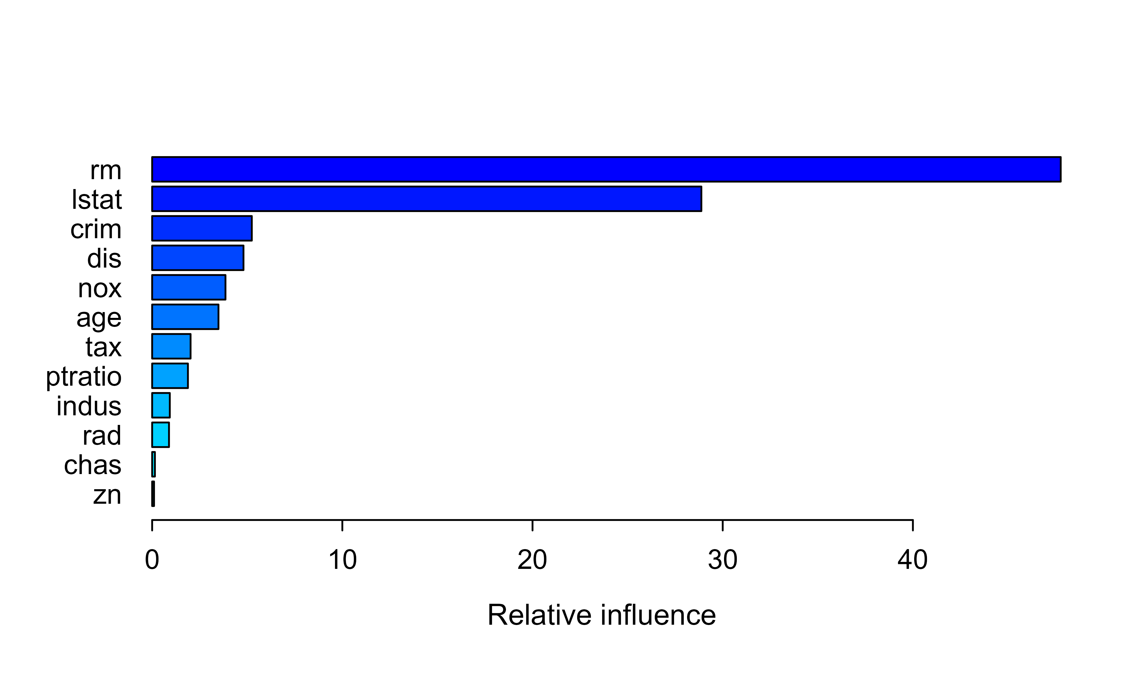
library(gbm)library(ISLR2)library(tree)set.seed(1)train<-sample(1:nrow(Boston), nrow(Boston)/2)boston.test<-Boston[-train, "medv"]boost.boston<-gbm(medv~., data =Boston[train, ], distribution ="gaussian", # because this is regression setting# distribution = "bernoulli", # use this for classification n.trees =5000, # number of trees interaction.depth =4# limits the depth of each tree)summary(boost.boston)#rm and lstate are most important#> var rel.inf#> rm rm 47.77218552#> lstat lstat 28.87780274#> crim crim 5.24064005#> dis dis 4.80273982#> nox nox 3.85568245#> age age 3.48748838#> tax tax 2.02093857#> ptratio ptratio 1.88187639#> indus indus 0.92881145#> rad rad 0.88654369#> chas chas 0.14576488#> zn zn 0.09952606
Figure 11.1: Relative influence of each predictor in the gbm boosted model for the Boston housing data, ranked from most to least important.
The summary() output ranks the variables by relative influence, shown in Figure 11.1. Here rm (average number of rooms) and lstat (percent lower-status population) dominate, which matches the intuition that house size and neighborhood drive price.
For a fuller workflow (tuning, visualization, and prediction), we follow an example by the University of Cincinnati3, using the larger Ames housing data set. First, we load the packages that support the workflow.
It is worth knowing the personality of the gbm implementation before we lean on it. The gbm package:
can handle up to 1024 factor levels,
supports many loss functions,
has no automated early stopping, and
offers internal cross-validation that can be combined with parallelization.
We split the Ames data into training (70%) and test (30%) sets, using a fixed seed so the results are reproducible.
Show code
# Create training (70%) and test (30%) sets for the AmesHousing::make_ames() data.# Use set.seed for reproducibilityset.seed(123)ames_split<-initial_split(AmesHousing::make_ames(), prop =.7)ames_train<-training(ames_split)ames_test<-testing(ames_split)
Now we fit a first model. Note the deliberately slow learning rate (shrinkage = 0.001) paired with a large number of trees (n.trees = 10000) and shallow stumps (interaction.depth = 1). The cv.folds = 5 argument turns on 5-fold cross-validation so we can read off how many trees we actually need.
Show code
# for reproducibilityset.seed(123)# train GBM modelgbm.fit<-gbm( formula =Sale_Price~., distribution ="gaussian", data =ames_train, n.trees =10000, interaction.depth =1, shrinkage =0.001, cv.folds =5, n.cores =NULL, # will use all cores by default verbose =FALSE)# print resultsprint(gbm.fit)#> gbm(formula = Sale_Price ~ ., distribution = "gaussian", data = ames_train, #> n.trees = 10000, interaction.depth = 1, shrinkage = 0.001, #> cv.folds = 5, verbose = FALSE, n.cores = NULL)#> A gradient boosted model with gaussian loss function.#> 10000 iterations were performed.#> The best cross-validation iteration was 10000.#> There were 80 predictors of which 45 had non-zero influence.
The cross-validation error tells us the best number of trees and, taking its square root, the cross-validated RMSE in dollars.
Show code
# get MSE and compute RMSEsqrt(min(gbm.fit$cv.error))#> [1] 28901.16## [1] 29133.33# plot loss function as a result of n trees added to the ensemblegbm.perf(gbm.fit, method ="cv")#> [1] 10000
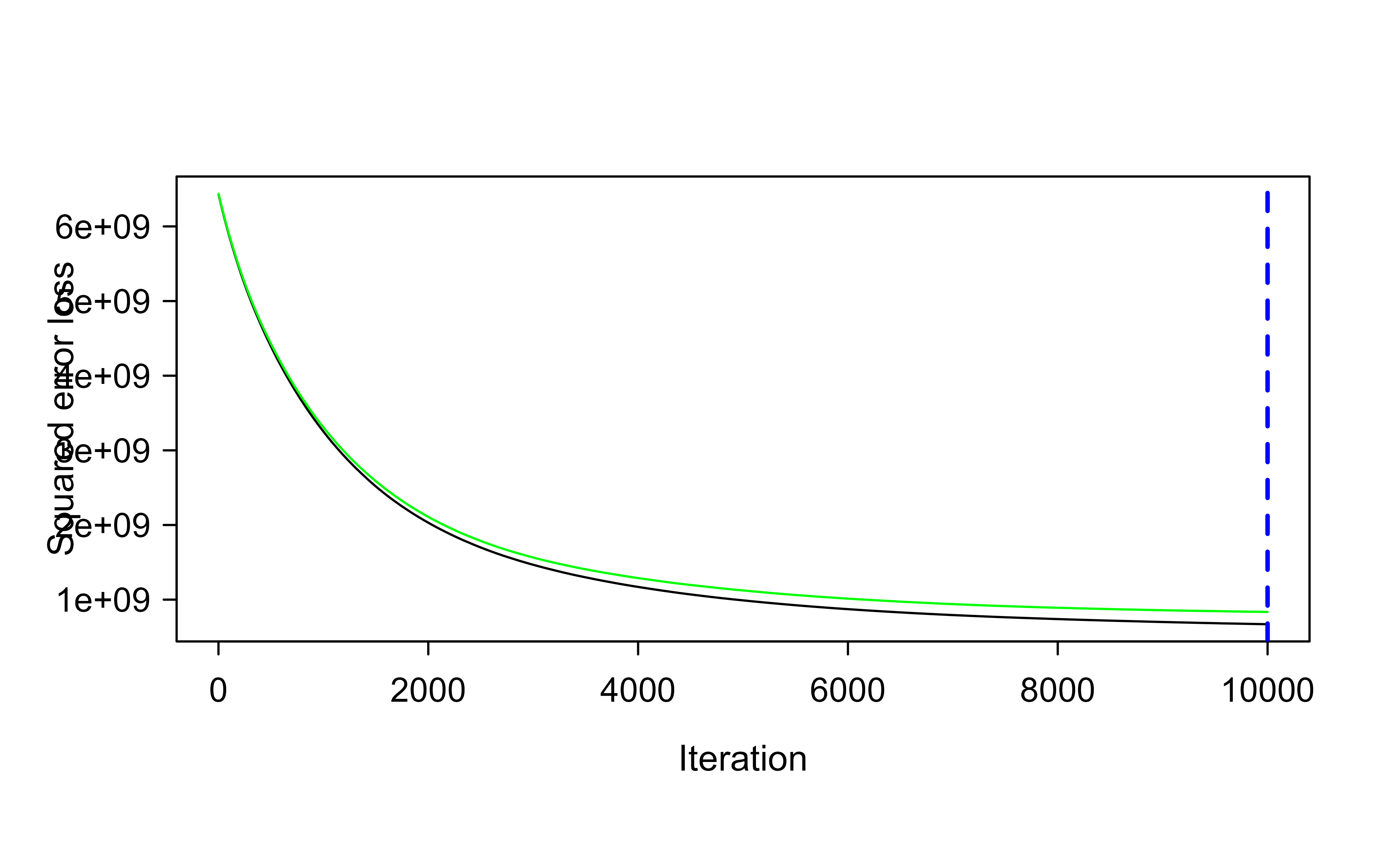
Figure 11.2: Cross-validated loss as a function of the number of trees for the slow-learning gbm fit on the Ames data, with the optimal number of trees marked by the dashed line.
Figure 11.2 shows the loss falling as trees are added, with the optimal point marked. Because the learning rate is so small, the curve is still descending after many thousands of trees: a small learning rate can demand a great many trees.
11.6.1.3 Tuning
Since a tiny learning rate forces a huge tree count, the natural next move is to trade some of that slowness for speed: raise the learning rate (which lets us use fewer trees) and let each tree be a little deeper. The following model uses shrinkage = 0.1 and interaction.depth = 3.
Show code
# for reproducibilityset.seed(123)# train GBM modelgbm.fit2<-gbm( formula =Sale_Price~., distribution ="gaussian", data =ames_train, n.trees =5000, interaction.depth =3, shrinkage =0.1, cv.folds =5, n.cores =NULL, # will use all cores by default verbose =FALSE)# find index for n trees with minimum CV errormin_MSE<-which.min(gbm.fit2$cv.error)# get MSE and compute RMSEsqrt(gbm.fit2$cv.error[min_MSE])#> [1] 22723.18## [1] 23112.1# plot loss function as a result of n trees added to the ensemblegbm.perf(gbm.fit2, method ="cv")#> [1] 818
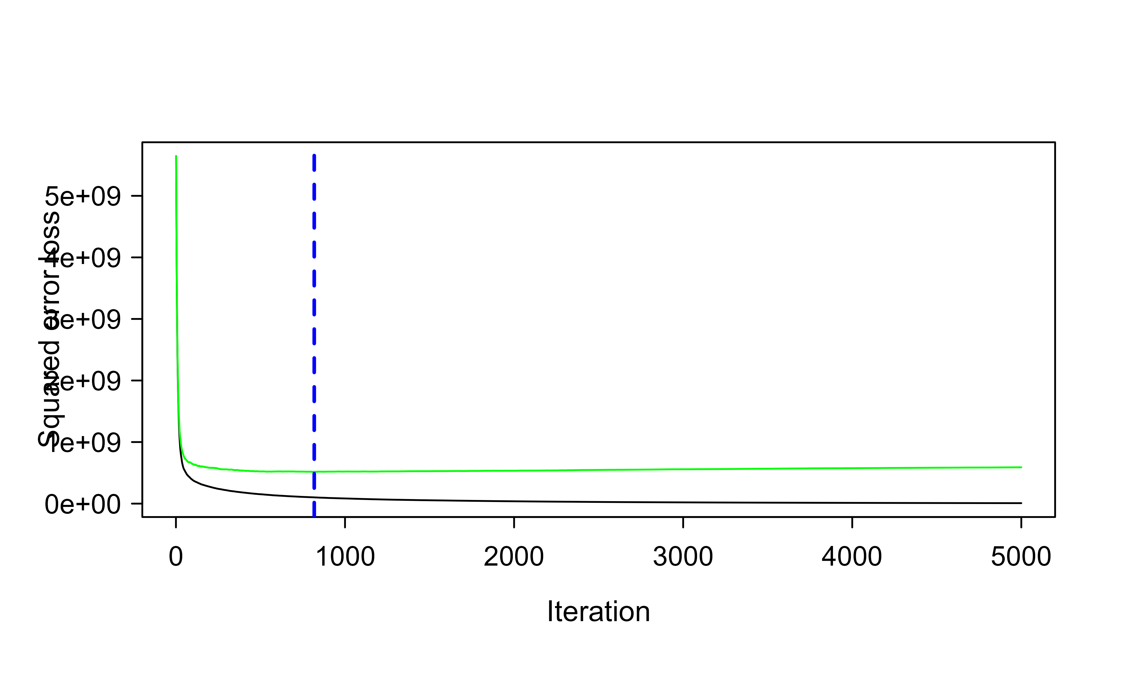
Figure 11.3: Cross-validated loss versus number of trees for the faster, deeper gbm fit (shrinkage 0.1, interaction depth 3) on the Ames data.
Figure 11.3 shows that the faster, deeper model reaches a noticeably lower cross-validated RMSE with far fewer trees. Tuning one parameter at a time like this is instructive, but in practice we search the parameter space jointly with a grid search.
Show code
# create hyperparameter gridhyper_grid<-expand.grid( shrinkage =c(.01, .1, .3), interaction.depth =c(1, 3, 5), n.minobsinnode =c(5, 10, 15), bag.fraction =c(.65, .8, 1), optimal_trees =0, # a place to dump results min_RMSE =0# a place to dump results)# total number of combinationsnrow(hyper_grid)#> [1] 81
Before running the (slow) search, it is worth knowing what patterns to expect in the results. From experience with this data:
the top models do not use a learning rate of 0.3 (small incremental steps usually work best),
the top models are not stumps (there are likely interactions that deeper trees can capture),
adding a stochastic component (bag.fraction < 1) tends to help (which hints at local minima in the loss gradient), and
the top models do not use a large minimum number of observations per node (n.minobsinnode = 15), so smaller nodes can capture pockets of unusual points.
The grid search itself loops over every combination, fits a model, and records the optimal number of trees and the validation RMSE. It is set to eval = FALSE here because it is slow to run.
Show code
# randomize datarandom_index<-sample(1:nrow(ames_train), nrow(ames_train))random_ames_train<-ames_train[random_index, ]# grid searchfor(iin1:nrow(hyper_grid)){# reproducibilityset.seed(123)# train modelgbm.tune<-gbm( formula =Sale_Price~., distribution ="gaussian", data =random_ames_train, n.trees =5000, interaction.depth =hyper_grid$interaction.depth[i], shrinkage =hyper_grid$shrinkage[i], n.minobsinnode =hyper_grid$n.minobsinnode[i], bag.fraction =hyper_grid$bag.fraction[i], train.fraction =.75, n.cores =NULL, # will use all cores by default verbose =FALSE)# add min training error and trees to gridhyper_grid$optimal_trees[i]<-which.min(gbm.tune$valid.error)hyper_grid$min_RMSE[i]<-sqrt(min(gbm.tune$valid.error))}hyper_grid%>%dplyr::arrange(min_RMSE)%>%head(10)
Having found a promising region, we can zoom in with a finer grid around the best values.
Show code
# modify hyperparameter gridhyper_grid<-expand.grid( shrinkage =c(.01, .05, .1), interaction.depth =c(3, 5, 7), n.minobsinnode =c(5, 7, 10), bag.fraction =c(.65, .8, 1), optimal_trees =0, # a place to dump results min_RMSE =0# a place to dump results)# total number of combinationsnrow(hyper_grid)
Then we repeat the search over the refined grid.
Show code
# grid searchfor(iin1:nrow(hyper_grid)){# reproducibilityset.seed(123)# train modelgbm.tune<-gbm( formula =Sale_Price~., distribution ="gaussian", data =random_ames_train, n.trees =6000, interaction.depth =hyper_grid$interaction.depth[i], shrinkage =hyper_grid$shrinkage[i], n.minobsinnode =hyper_grid$n.minobsinnode[i], bag.fraction =hyper_grid$bag.fraction[i], train.fraction =.75, n.cores =NULL, # will use all cores by default verbose =FALSE)# add min training error and trees to gridhyper_grid$optimal_trees[i]<-which.min(gbm.tune$valid.error)hyper_grid$min_RMSE[i]<-sqrt(min(gbm.tune$valid.error))}hyper_grid%>%dplyr::arrange(min_RMSE)%>%head(10)
Once the search identifies the best combination, we retrain a single final model on the full training set using those parameters.
Show code
# for reproducibilityset.seed(123)# train GBM modelgbm.fit.final<-gbm( formula =Sale_Price~., distribution ="gaussian", data =ames_train, n.trees =483, interaction.depth =5, shrinkage =0.1, n.minobsinnode =5, bag.fraction =.65, train.fraction =1, n.cores =NULL, # will use all cores by default verbose =FALSE)
11.6.1.4 Visualization
A trained boosting model is accurate but, on its own, opaque. The next few tools turn it back into something a human can reason about: which variables matter, how each variable affects the prediction, and why a particular prediction came out the way it did. These model-agnostic methods are treated more fully in the interpretable machine learning chapter (Chapter 35).
11.6.1.4.1 Variable importance
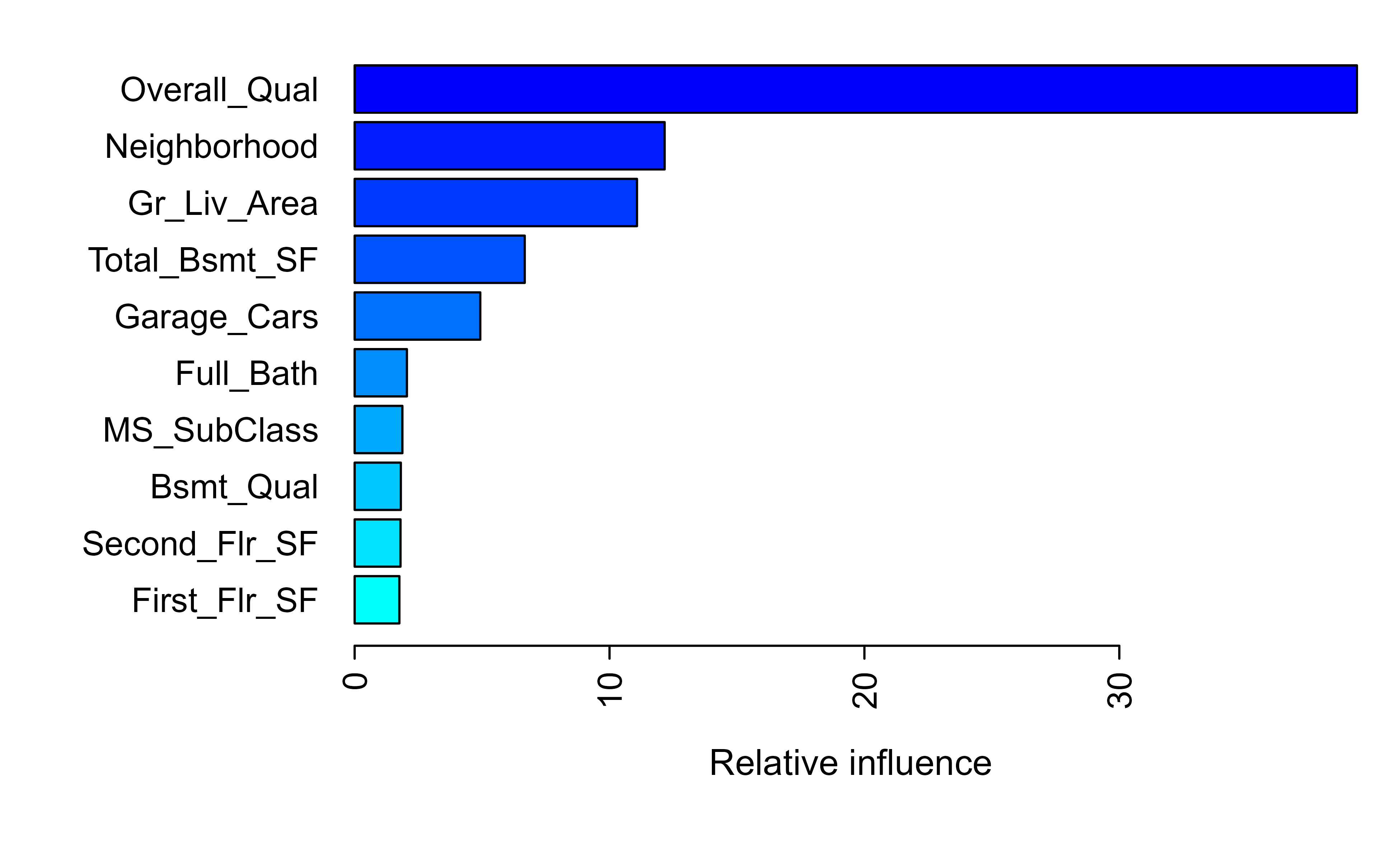
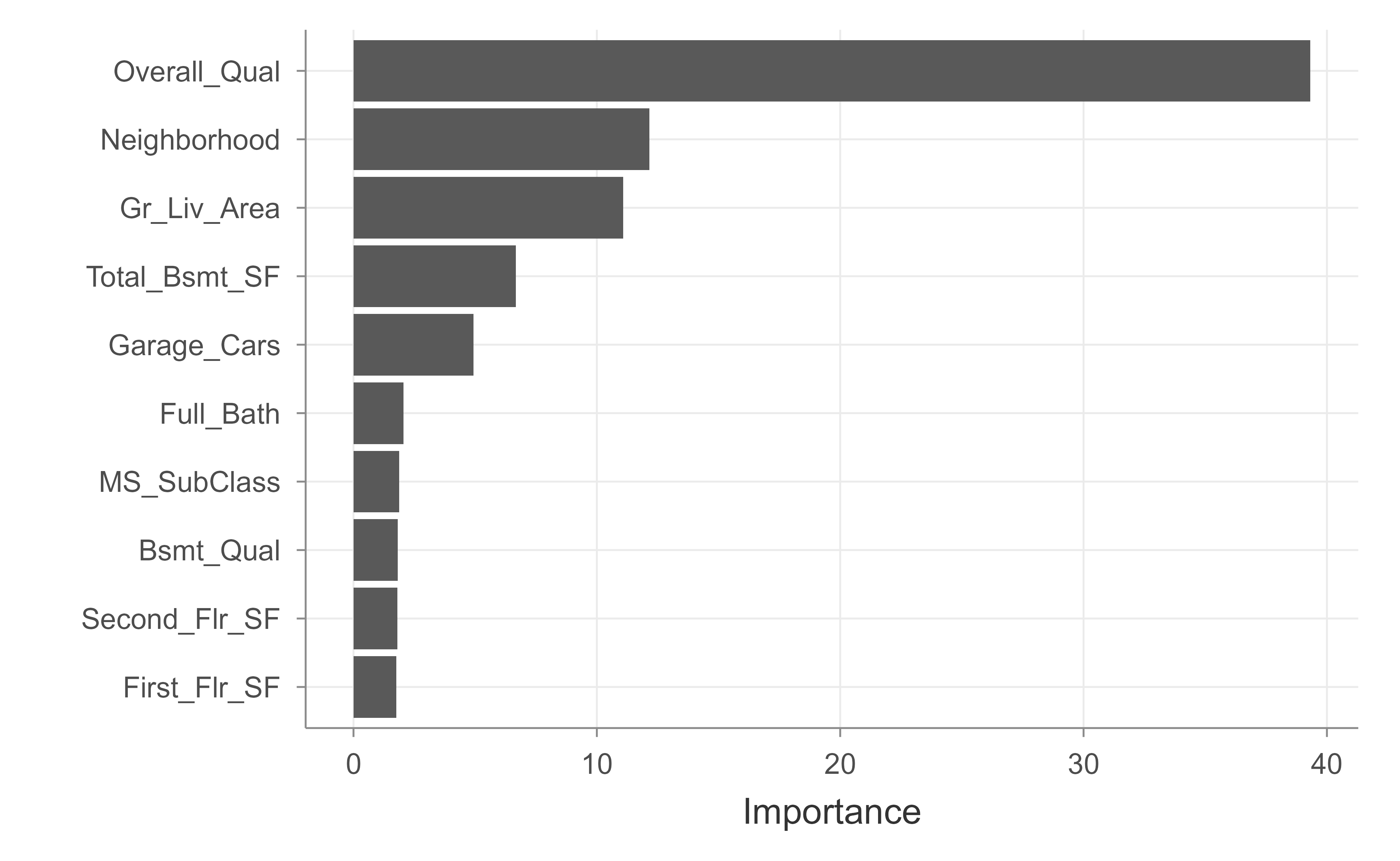
The first question is usually: which variable has the largest influence on the response? The summary() method answers this by relative influence, as plotted in Figure 11.4.
Figure 11.4: Relative influence of the top predictors in the final tuned gbm model for the Ames housing data.
The vip package produces a similar ranking with a cleaner default plot, shown in Figure 11.5.
Show code
vip::vip(gbm.fit.final)
Figure 11.5: Variable importance for the final tuned gbm model, produced by the vip package.
11.6.1.4.2 Partial dependence plots
Variable importance tells you which variables matter but not how. Partial dependence plots (PDPs) and individual conditional expectation (ICE) curves fill that gap:
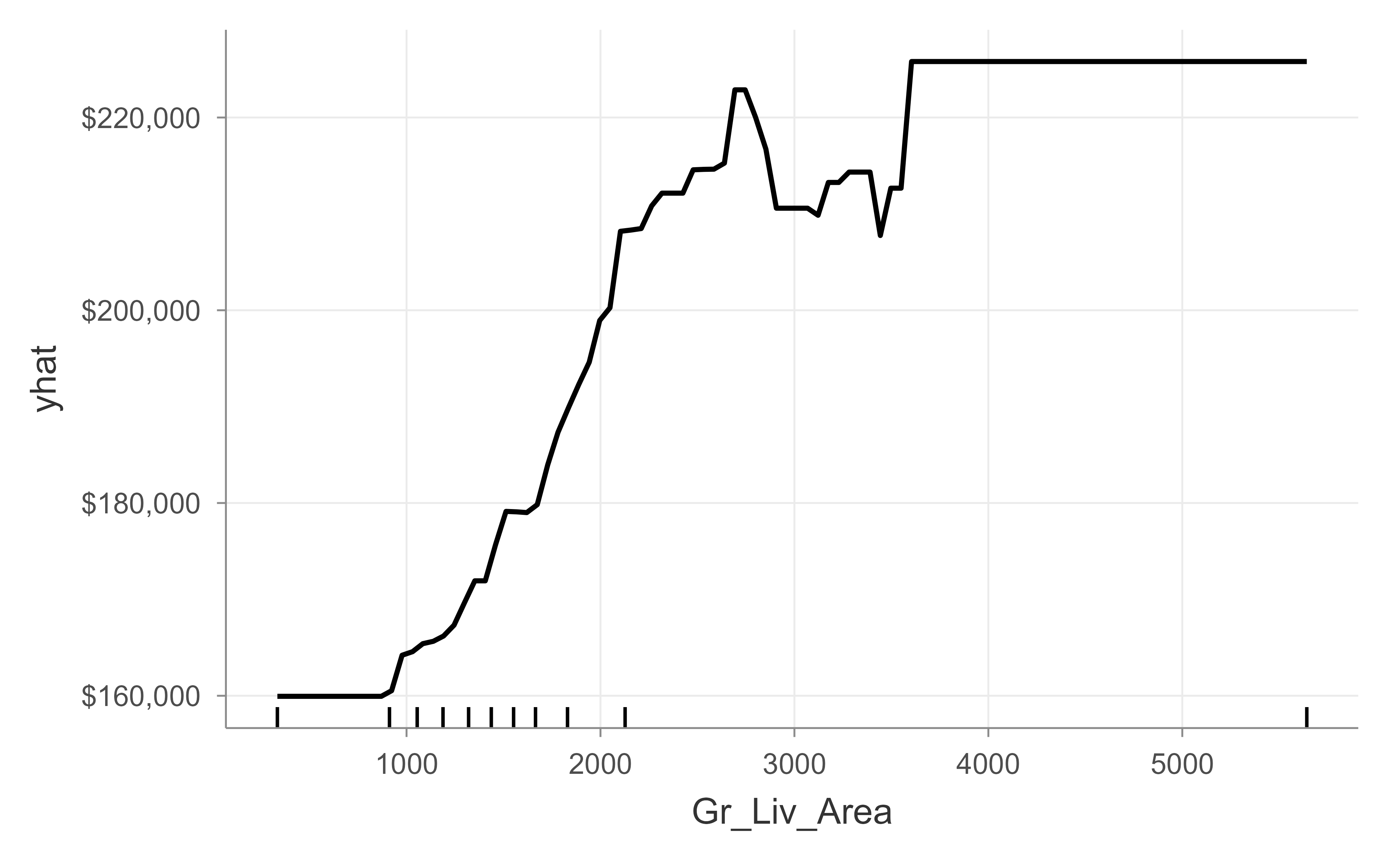
PDPs show how the average prediction changes as a feature varies over its range, averaging out the other features.
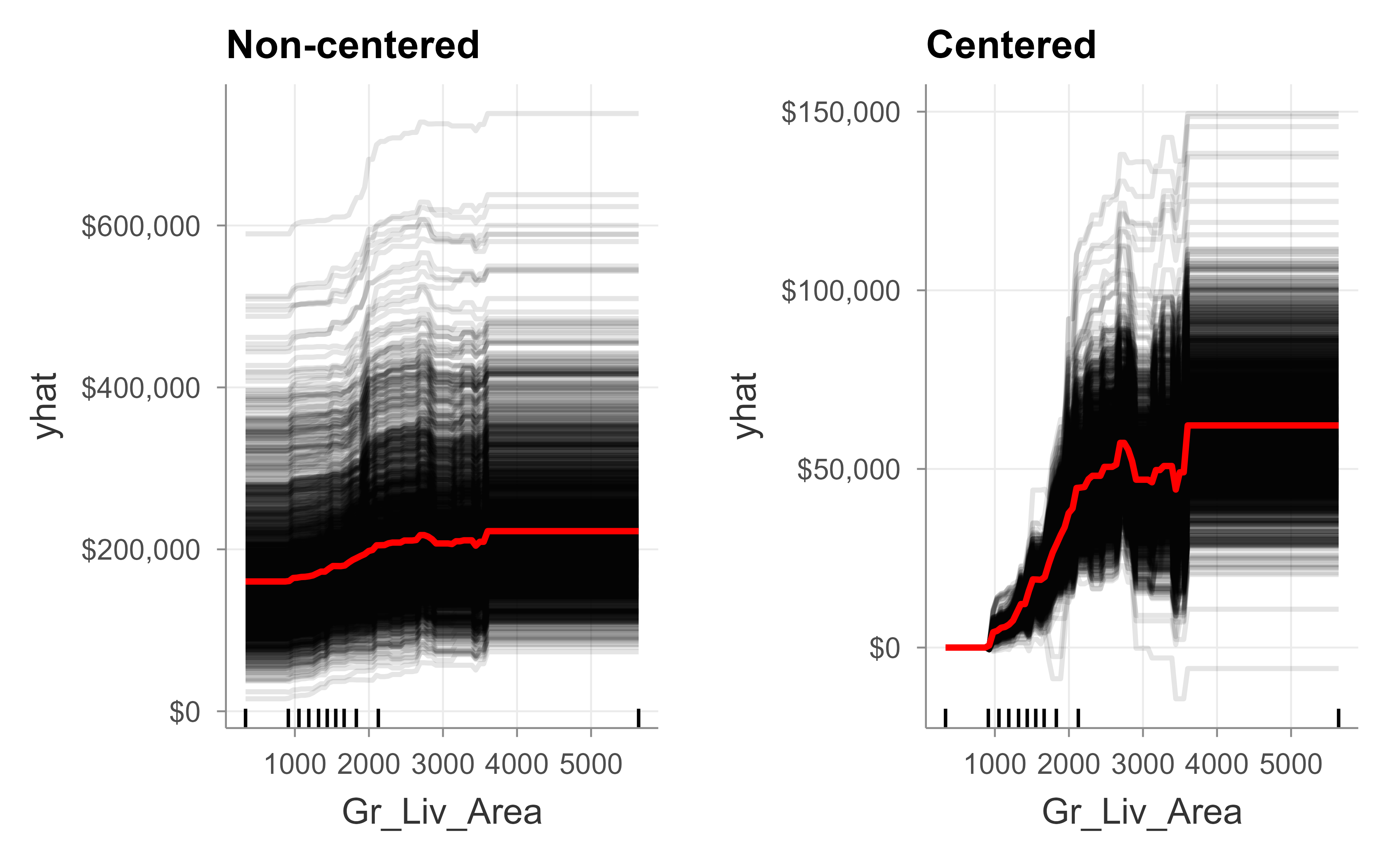
ICE curves are an extension that shows the same thing for each observation separately, which can reveal interactions that the averaged PDP hides.
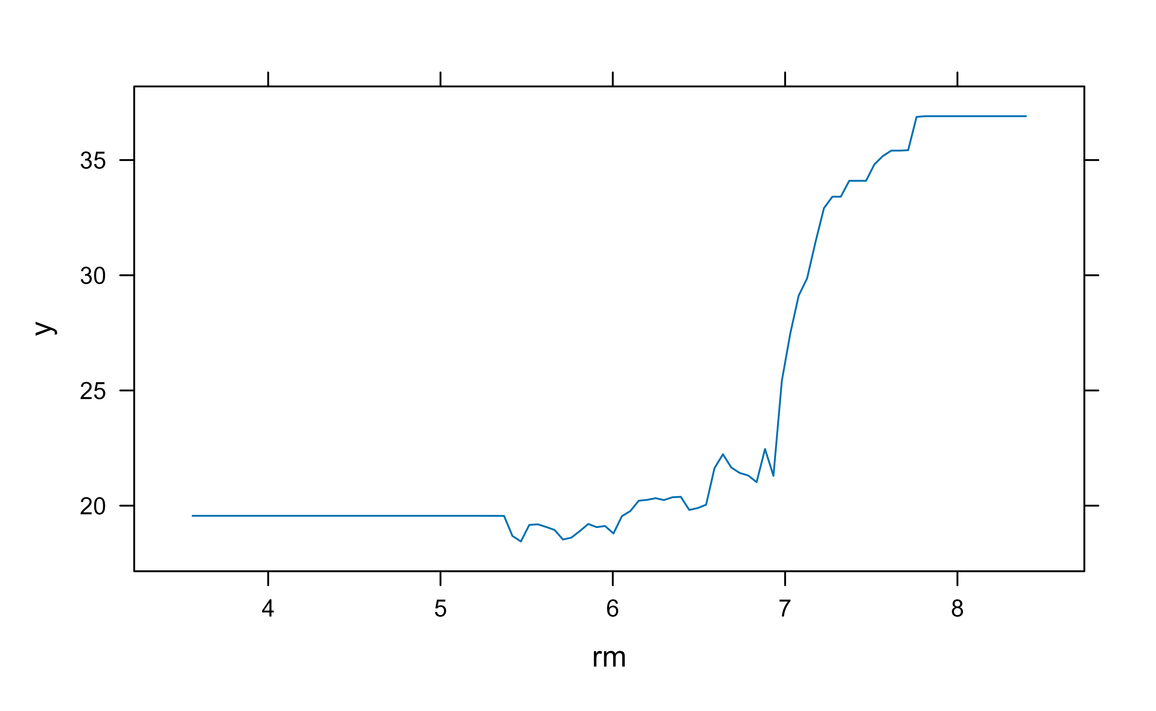
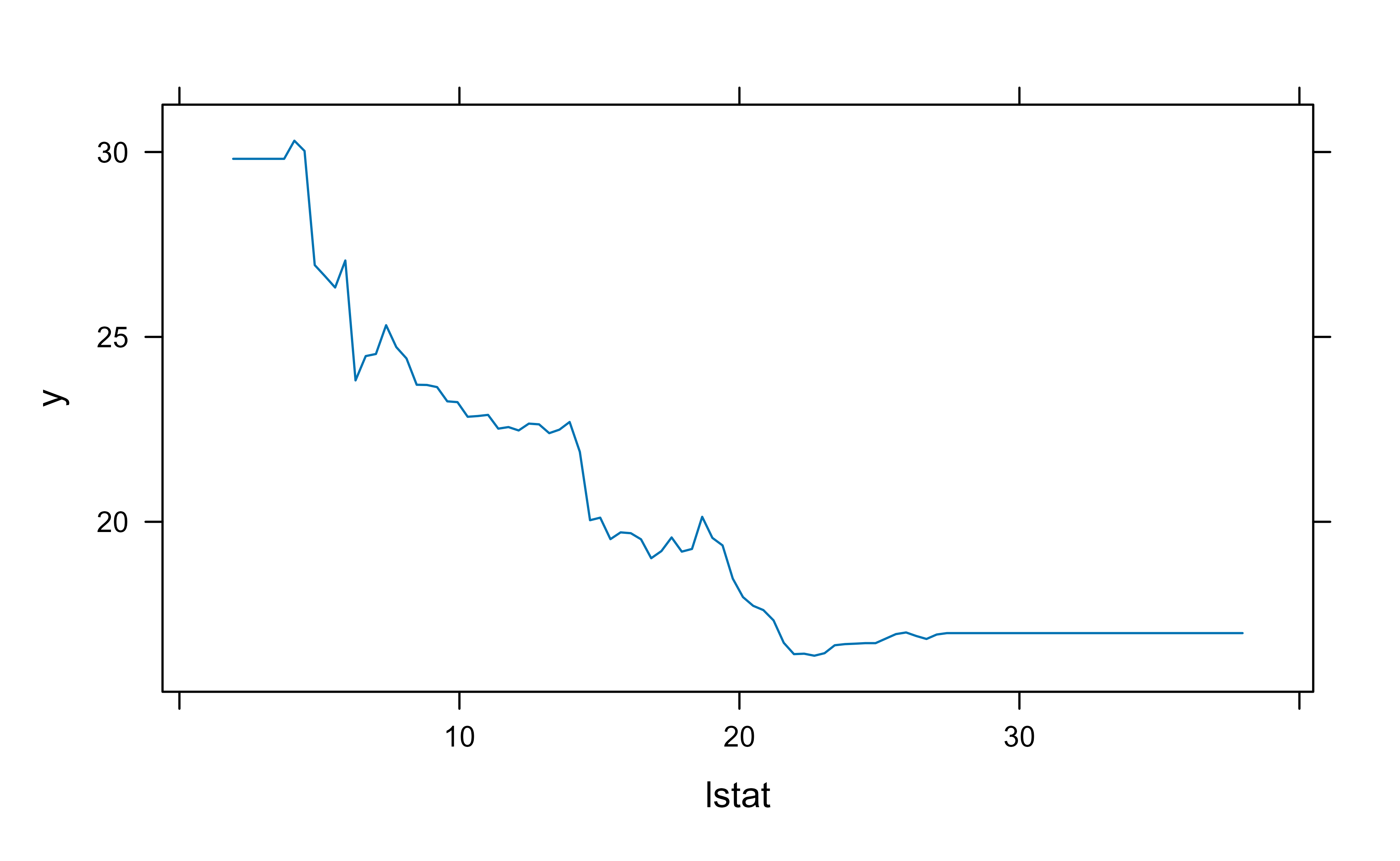
The PDP in Figure 11.6 shows how predicted sale price rises with above-grade living area.
Figure 11.6: Partial dependence of predicted sale price on above-grade living area (Gr_Liv_Area) for the final gbm model.
Figure 11.7 draws the ICE curves, both in their raw form and centered so every curve starts at the same point, which makes differences in slope easier to compare.
Figure 11.7: Individual conditional expectation curves for above-grade living area, shown non-centered (left) and centered (right) for the final gbm model.
11.6.1.4.3 LIME
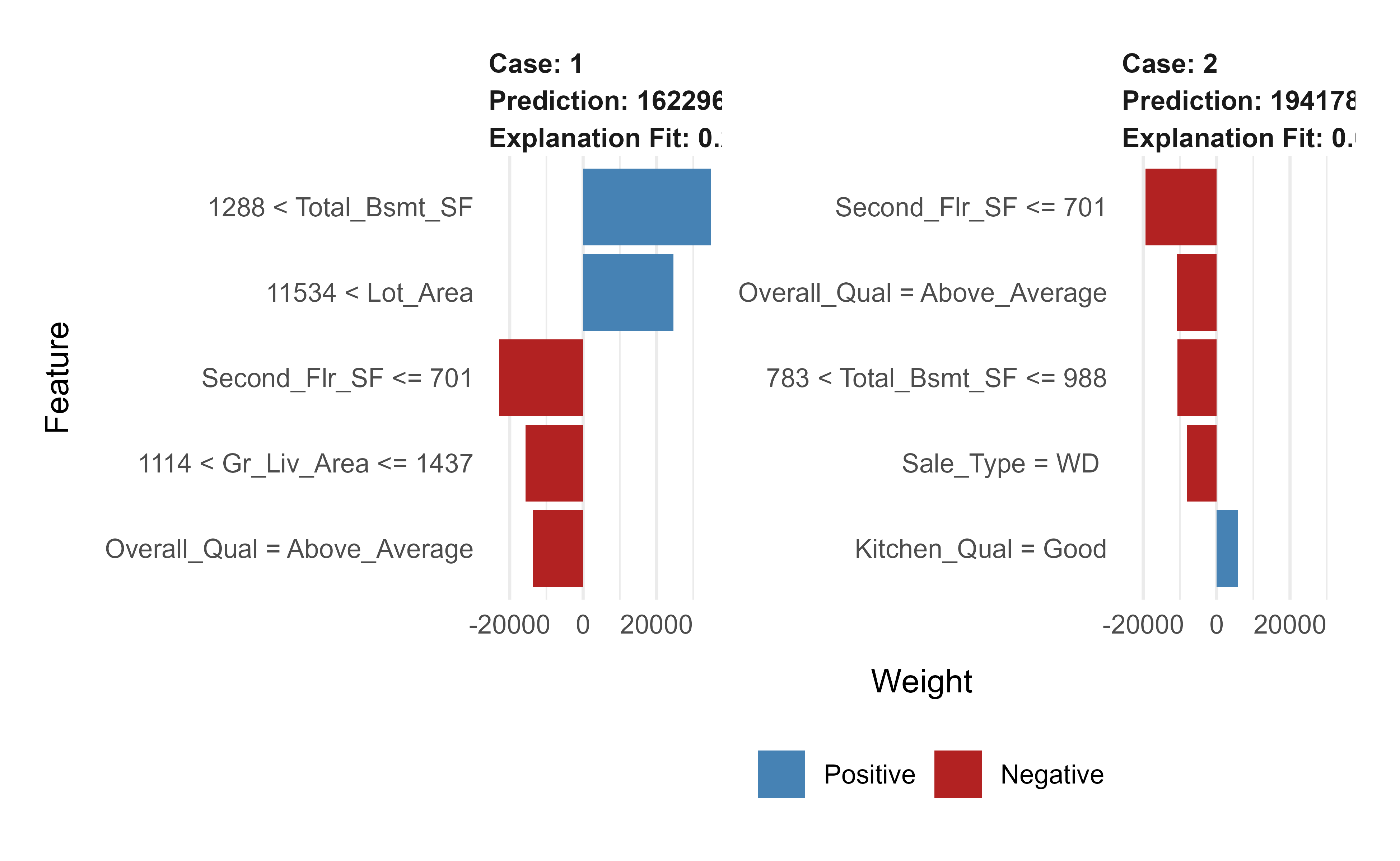
PDPs and ICE describe the model globally. LIME (Local Interpretable Model-agnostic Explanations) answers a different, local question: why did the model produce this particular prediction for this particular house? It does so by fitting a simple, interpretable model in the neighborhood of the observation you care about.
To use LIME with a gbm object, we first tell it that this model does regression and how to get predictions out of it.
Below we call lime::lime() and lime::explain() with their package prefixes. The name explain is also defined by dplyr, so prefixing avoids a masking conflict that would otherwise break the call when both packages are loaded.
Show code
# get a few observations to perform local interpretation onlocal_obs<-ames_test[1:2, ]# apply LIMEexplainer<-lime::lime(ames_train, gbm.fit.final)explanation<-lime::explain(local_obs, explainer, n_features =5)plot_features(explanation)
Figure 11.8: LIME local explanations for two test observations under the final gbm model, showing the features that most influenced each individual prediction.
Each bar in Figure 11.8 shows how much a feature pushed that specific prediction up or down, which is exactly the kind of explanation you would want to give a stakeholder.
11.6.1.5 Prediction
Finally, the payoff: predictions on held-out data, scored by RMSE.
Show code
# predict values for test datapred<-predict(gbm.fit.final, n.trees =gbm.fit.final$n.trees, ames_test)# resultscaret::RMSE(pred, ames_test$Sale_Price)#> [1] 21365.24
11.6.2 Gradient Boost Classification
The classification version of the algorithm is structurally identical to the regression one; only the loss function changes. For binary classification we use the negative log-likelihood (deviance), which is differentiable and so fits cleanly into the gradient framework.
Input: Data \(\{(x_i, y_i)\}^n_{i=1}\) and a differentiable Loss Function \(L(y_i, F(x))\) (e.g., Classification: negative log likelihood: \(-\sum_{i=1}^N \big[\, y_i \log(p_i) + (1 - y_i)\log(1 - p_i) \,\big]\) where \(y_i\) is the observed value and \(p_i\) the predicted probability for observation \(i\), equivalently, \(-\sum_{i=1}^N \big[\, \text{Observed}_i \times \log(\text{odds}_i) + \log\!\big(1 + \exp(\log(\text{odds}_i))\big) \,\big]\) which is differentiable)
Step 1: Initialize model with a constant value: \(F_0(x) = \underset{\gamma}{\operatorname{argmin}} \sum_{i=1}^n L(y_i, \gamma)\) where \(\gamma\) is a log(odds) value
Step 2: for \(m = 1 \to M\) (number of trees):
Compute the (pseudo) residual: \(r_{im} = - [ \frac{\partial L( y_i, F(x_i))}{\partial F(x_i)}]_{F(x) = F_{m-1}(x)}\) for \(i = 1, \dots, n\) (where \(\frac{\partial L( y_i, F(x_i))}{\partial F(x_i)}\) is the gradient, ergo the name gradient boost)
Fit a regression tree to the \(r_{im}\) values and create terminal regions \(R_{jm}\) for \(j = 1, \dots, J_m\)
Update \(F_m (x) = F_{m-1}(x) + \nu \sum_{j=1}^{J_m} \gamma_{jm} I(x \in R_{jm})\) where \(\nu\) is the learning rate (0 to 1) (smaller value means slower learning rate)
Output: \(F_M(x)\)
Because the model works in log-odds space, the optimal leaf value in step 2.3 has a convenient closed form for this loss:
The numerator pulls the leaf toward the residuals; the denominator, built from the current predicted probabilities, damps the step where the model is already confident.
This closed form is a direct instance of the Newton leaf value in Equation 11.6. Work in log-odds space, \(F(x) = \log\frac{p(x)}{1 - p(x)}\), so that \(p = \sigma(F) = 1/(1 + e^{-F})\), and code \(y \in \{0, 1\}\). The per-observation deviance is
\[
L(y, F) = -\big[\, y F - \log(1 + e^{F}) \,\big],
\]
obtained by writing the Bernoulli log-likelihood \(y \log p + (1-y)\log(1-p)\) in terms of \(F\). Its first derivative is
which is precisely the formula above. The same calculation explains the initial value in step 1: minimizing \(\sum_i L(y_i, \gamma)\) over a constant \(\gamma\) gives \(\sigma(\gamma) = \bar{y}\), so \(F_0 = \log\frac{\bar y}{1 - \bar y}\) is the global log-odds of the positive class.
11.7 Stochastic Gradient Boosting
So far each tree has seen all of the data. Stochastic gradient boosting borrows the randomness that made bagging (Chapter 10) and random forests (Chapter 13) effective: by fitting each tree to a random subsample, we reduce the correlation between successive trees in the boosting sequence, which often improves generalization.
Two common forms of subsampling are:
subsample rows (and/or columns) before creating each tree, and
subsample columns before each split.
Tip
Setting the row subsample fraction below 1 (the bag.fraction argument in gbm) is a cheap and reliable regularizer. It is one of the first knobs to try when a boosted model overfits.
11.8 Penalized Gradient Boosting
Another way to control complexity is to penalize the tree parameters directly. L1 regularization (Lasso, Chapter 1) and L2 regularization (Ridge, Chapter 1) can both be imposed on the weights inside the trees, shrinking them toward zero and discouraging overly elaborate fits. This is part of what the “regularized boosting” in XGBoost refers to.
11.9 Light Gradient Boosting
As data sets grow, the cost of scanning every observation and every feature at each split becomes the bottleneck. LightGBM (references: Machado, Karray, and de Sousa (2019) and the original paper4) attacks that bottleneck with two ideas:
Gradient-based One-Side Sampling (GOSS): a modification of gradient boosting that keeps the training examples with large gradients (the ones the model still gets most wrong) and subsamples the rest, which speeds up learning.
Exclusive Feature Bundling (EFB): bundling sparse, mostly-zero features that are rarely nonzero at the same time, a form of automatic feature selection that shrinks the effective number of features.
Together these give LightGBM its characteristic profile:
faster and more efficient training,
lower memory use,
often better accuracy,
support for parallel, distributed, and GPU learning,
For details, see the function reference5. The following example, adapted from the LightGBM documentation6, runs cross-validation on the bundled mushroom data.
Show code
library(lightgbm)data(agaricus.train, package='lightgbm')train<-agaricus.traindtrain<-lgb.Dataset(train$data, label =train$label)model<-lgb.cv( params =list( objective ="regression" , metric ="l2") , data =dtrain)#> [LightGBM] [Info] Auto-choosing row-wise multi-threading, the overhead of testing was 0.004130 seconds.#> You can set `force_row_wise=true` to remove the overhead.#> And if memory is not enough, you can set `force_col_wise=true`.#> [LightGBM] [Info] Total Bins 214#> [LightGBM] [Info] Number of data points in the train set: 4342, number of used features: 107#> [LightGBM] [Info] Auto-choosing row-wise multi-threading, the overhead of testing was 0.003976 seconds.#> You can set `force_row_wise=true` to remove the overhead.#> And if memory is not enough, you can set `force_col_wise=true`.#> [LightGBM] [Info] Total Bins 214#> [LightGBM] [Info] Number of data points in the train set: 4342, number of used features: 107#> [LightGBM] [Info] Auto-choosing row-wise multi-threading, the overhead of testing was 0.004252 seconds.#> You can set `force_row_wise=true` to remove the overhead.#> And if memory is not enough, you can set `force_col_wise=true`.#> [LightGBM] [Info] Total Bins 214#> [LightGBM] [Info] Number of data points in the train set: 4342, number of used features: 107#> [LightGBM] [Info] Start training from score 0.479272#> [LightGBM] [Warning] No further splits with positive gain, best gain: -inf#> [LightGBM] [Info] Start training from score 0.481345#> [LightGBM] [Warning] No further splits with positive gain, best gain: -inf#> [LightGBM] [Info] Start training from score 0.485721#> [LightGBM] [Warning] No further splits with positive gain, best gain: -inf#> [1]: valid's l2:0.202944+0.000532057 #> [LightGBM] [Warning] No further splits with positive gain, best gain: -inf#> [LightGBM] [Warning] No further splits with positive gain, best gain: -inf#> [LightGBM] [Warning] No further splits with positive gain, best gain: -inf#> [2]: valid's l2:0.165052+0.000832598 #> [LightGBM] [Warning] No further splits with positive gain, best gain: -inf#> [LightGBM] [Warning] No further splits with positive gain, best gain: -inf#> [LightGBM] [Warning] No further splits with positive gain, best gain: -inf#> [3]: valid's l2:0.134166+0.000791853 #> [LightGBM] [Warning] No further splits with positive gain, best gain: -inf#> [LightGBM] [Warning] No further splits with positive gain, best gain: -inf#> [LightGBM] [Warning] No further splits with positive gain, best gain: -inf#> [4]: valid's l2:0.109125+0.000762195 #> [LightGBM] [Warning] No further splits with positive gain, best gain: -inf#> [LightGBM] [Warning] No further splits with positive gain, best gain: -inf#> [LightGBM] [Warning] No further splits with positive gain, best gain: -inf#> [5]: valid's l2:0.0888474+0.000741643 #> [LightGBM] [Warning] No further splits with positive gain, best gain: -inf#> [LightGBM] [Warning] No further splits with positive gain, best gain: -inf#> [LightGBM] [Warning] No further splits with positive gain, best gain: -inf#> [6]: valid's l2:0.0724021+0.000731231 #> [LightGBM] [Warning] No further splits with positive gain, best gain: -inf#> [LightGBM] [Warning] No further splits with positive gain, best gain: -inf#> [7]: valid's l2:0.0590889+0.00073343 #> [LightGBM] [Warning] No further splits with positive gain, best gain: -inf#> [LightGBM] [Warning] No further splits with positive gain, best gain: -inf#> [8]: valid's l2:0.0482839+0.000740685 #> [LightGBM] [Warning] No further splits with positive gain, best gain: -inf#> [LightGBM] [Warning] No further splits with positive gain, best gain: -inf#> [9]: valid's l2:0.0395356+0.000738131 #> [LightGBM] [Warning] No further splits with positive gain, best gain: -inf#> [LightGBM] [Warning] No further splits with positive gain, best gain: -inf#> [10]: valid's l2:0.032444+0.000741093 #> [LightGBM] [Warning] No further splits with positive gain, best gain: -inf#> [LightGBM] [Warning] No further splits with positive gain, best gain: -inf#> [11]: valid's l2:0.026648+0.000788356 #> [LightGBM] [Warning] No further splits with positive gain, best gain: -inf#> [LightGBM] [Warning] No further splits with positive gain, best gain: -inf#> [12]: valid's l2:0.0219544+0.000825051 #> [LightGBM] [Warning] No further splits with positive gain, best gain: -inf#> [LightGBM] [Warning] No further splits with positive gain, best gain: -inf#> [13]: valid's l2:0.0180945+0.000883922 #> [LightGBM] [Warning] No further splits with positive gain, best gain: -inf#> [14]: valid's l2:0.0149173+0.000865451 #> [LightGBM] [Warning] No further splits with positive gain, best gain: -inf#> [LightGBM] [Warning] No further splits with positive gain, best gain: -inf#> [15]: valid's l2:0.0123778+0.000895705 #> [LightGBM] [Warning] No further splits with positive gain, best gain: -inf#> [16]: valid's l2:0.0102813+0.000872654 #> [LightGBM] [Warning] No further splits with positive gain, best gain: -inf#> [17]: valid's l2:0.00857126+0.000861128 #> [18]: valid's l2:0.00720567+0.000880488 #> [LightGBM] [Warning] No further splits with positive gain, best gain: -inf#> [19]: valid's l2:0.00606723+0.00084912 #> [LightGBM] [Warning] No further splits with positive gain, best gain: -inf#> [20]: valid's l2:0.00513746+0.000813256 #> [LightGBM] [Warning] No further splits with positive gain, best gain: -inf#> [21]: valid's l2:0.00437427+0.000780301 #> [LightGBM] [Warning] No further splits with positive gain, best gain: -inf#> [22]: valid's l2:0.00374844+0.000746947 #> [LightGBM] [Warning] No further splits with positive gain, best gain: -inf#> [23]: valid's l2:0.00323359+0.000714182 #> [LightGBM] [Warning] No further splits with positive gain, best gain: -inf#> [24]: valid's l2:0.00280815+0.000682128 #> [LightGBM] [Warning] No further splits with positive gain, best gain: -inf#> [25]: valid's l2:0.00245573+0.000651835 #> [LightGBM] [Warning] No further splits with positive gain, best gain: -inf#> [26]: valid's l2:0.00216433+0.000618237 #> [27]: valid's l2:0.001926+0.000586016 #> [28]: valid's l2:0.00174254+0.000564653 #> [29]: valid's l2:0.00157368+0.000535848 #> [30]: valid's l2:0.0014322+0.000506773 #> [31]: valid's l2:0.0013188+0.000477638 #> [32]: valid's l2:0.00121741+0.00045024 #> [33]: valid's l2:0.00114196+0.000437478 #> [34]: valid's l2:0.00106355+0.000413461 #> [35]: valid's l2:0.000996203+0.000389535 #> [36]: valid's l2:0.000943046+0.000366316 #> [37]: valid's l2:0.000892934+0.000344205 #> [38]: valid's l2:0.000857363+0.000334656 #> [39]: valid's l2:0.000820203+0.000313447 #> [40]: valid's l2:0.000786204+0.000294331 #> [41]: valid's l2:0.000748499+0.000281854 #> [42]: valid's l2:0.000725595+0.000274276 #> [43]: valid's l2:0.000688456+0.000254103 #> [44]: valid's l2:0.000662856+0.000236656 #> [45]: valid's l2:0.000629943+0.00022819 #> [46]: valid's l2:0.000602124+0.000213556 #> [47]: valid's l2:0.000570399+0.000207722 #> [48]: valid's l2:0.000542492+0.000203123 #> [49]: valid's l2:0.000519129+0.000195094 #> [50]: valid's l2:0.000496565+0.000190158 #> [51]: valid's l2:0.000472076+0.000186775 #> [52]: valid's l2:0.000453739+0.000181817 #> [53]: valid's l2:0.000432198+0.000177771 #> [54]: valid's l2:0.000417528+0.000172524 #> [55]: valid's l2:0.000396702+0.000165251 #> [56]: valid's l2:0.000381477+0.000158046 #> [57]: valid's l2:0.000367827+0.000152129 #> [58]: valid's l2:0.000353074+0.000147805 #> [59]: valid's l2:0.000339696+0.000140022 #> [60]: valid's l2:0.000326833+0.000137771 #> [61]: valid's l2:0.000316935+0.000135149 #> [62]: valid's l2:0.000307284+0.000132574 #> [63]: valid's l2:0.000297724+0.000129215 #> [64]: valid's l2:0.000288992+0.000126218 #> [65]: valid's l2:0.000280951+0.000123581 #> [66]: valid's l2:0.000272885+0.000121291 #> [67]: valid's l2:0.000264758+0.000117979 #> [68]: valid's l2:0.000258181+0.00011594 #> [69]: valid's l2:0.000250816+0.000114211 #> [70]: valid's l2:0.000242199+0.00011169 #> [71]: valid's l2:0.00023481+0.000108103 #> [72]: valid's l2:0.000228397+0.000106477 #> [73]: valid's l2:0.000221714+0.000104317 #> [74]: valid's l2:0.000216673+0.000103814 #> [75]: valid's l2:0.000210542+0.000100825 #> [76]: valid's l2:0.000205102+9.91951e-05 #> [77]: valid's l2:0.000200624+9.77394e-05 #> [78]: valid's l2:0.000194036+9.52403e-05 #> [79]: valid's l2:0.000189553+9.34184e-05 #> [80]: valid's l2:0.000184529+9.06952e-05 #> [81]: valid's l2:0.000179209+8.99653e-05 #> [82]: valid's l2:0.000175319+8.88804e-05 #> [83]: valid's l2:0.000169749+8.64917e-05 #> [84]: valid's l2:0.00016608+8.52423e-05 #> [85]: valid's l2:0.000160898+8.28234e-05 #> [86]: valid's l2:0.000156855+8.18047e-05 #> [87]: valid's l2:0.000152762+7.95376e-05 #> [88]: valid's l2:0.000148613+7.87317e-05 #> [89]: valid's l2:0.000145702+7.81328e-05 #> [90]: valid's l2:0.000141627+7.62107e-05 #> [91]: valid's l2:0.0001387+7.46549e-05 #> [92]: valid's l2:0.000134596+7.24604e-05 #> [93]: valid's l2:0.000131336+7.12913e-05 #> [94]: valid's l2:0.000128512+7.08348e-05 #> [95]: valid's l2:0.000125506+6.95317e-05 #> [96]: valid's l2:0.000122127+6.83991e-05 #> [97]: valid's l2:0.000118863+6.64424e-05 #> [98]: valid's l2:0.000116347+6.52313e-05 #> [99]: valid's l2:0.000113949+6.41804e-05 #> [100]: valid's l2:0.000111944+6.34268e-05
The next example, from GeeksforGeeks7, is in Python and compares XGBoost against LightGBM on the adult-income data set (data link8).
Note
The Python comparison below is set to eval = FALSE. It depends on a Python environment with lightgbm, xgboost, pandas, and scikit-learn installed (via reticulate) and on a local copy of the images/adult.data file, which are not guaranteed in the build environment. The code is correct and idiomatic; run it locally after installing those packages.
#importing standard librariesimport numpy as npimport pandas as pdfrom pandas import Series, DataFrame#import lightgbm and xgboostimport lightgbm as lgbimport xgboost as xgb#loading our training dataset 'adult.csv' with name 'data' using pandasdata=pd.read_csv('images/adult.data',header=None)#Assigning names to the columnsdata.columns=['age','workclass','fnlwgt','education','education-num','marital_Status','occupation','relationship','race','sex','capital_gain','capital_loss','hours_per_week','native_country','Income']#glimpse of the datasetdata.head()# Label Encoding our target variablefrom sklearn.preprocessing import LabelEncoder,OneHotEncoderl=LabelEncoder()l.fit(data.Income)l.classes_data.Income=Series(l.transform(data.Income)) #label encoding our target variabledata.Income.value_counts()#One Hot Encoding of the Categorical featuresone_hot_workclass=pd.get_dummies(data.workclass)one_hot_education=pd.get_dummies(data.education)one_hot_marital_Status=pd.get_dummies(data.marital_Status)one_hot_occupation=pd.get_dummies(data.occupation)one_hot_relationship=pd.get_dummies(data.relationship)one_hot_race=pd.get_dummies(data.race)one_hot_sex=pd.get_dummies(data.sex)one_hot_native_country=pd.get_dummies(data.native_country)#removing categorical featuresdata.drop(['workclass','education','marital_Status','occupation','relationship','race','sex','native_country'],axis=1,inplace=True)#Merging one hot encoded features with our dataset 'data'data=pd.concat([data,one_hot_workclass,one_hot_education,one_hot_marital_Status,one_hot_occupation,one_hot_relationship,one_hot_race,one_hot_sex,one_hot_native_country],axis=1)#removing duplicate columns_, i = np.unique(data.columns, return_index=True)data=data.iloc[:, i]#Here our target variable is 'Income' with values as 1 or 0.#Separating our data into features dataset x and our target dataset yx=data.drop('Income',axis=1)y=data.Income#Imputing missing values in our target variabley.fillna(y.mode()[0],inplace=True)#Now splitting our dataset into test and trainfrom sklearn.model_selection import train_test_splitx_train,x_test,y_train,y_test=train_test_split(x,y,test_size=.3)#The data is stored in a DMatrix object#label is used to define our outcome variabledtrain=xgb.DMatrix(x_train,label=y_train)dtest=xgb.DMatrix(x_test)#setting parameters for xgboostparameters={'max_depth':7, 'eta':1, 'silent':1,'objective':'binary:logistic','eval_metric':'auc','learning_rate':.05}#training our modelnum_round=50from datetime import datetimestart = datetime.now()xg=xgb.train(parameters,dtrain,num_round)stop = datetime.now()#Execution time of the modelexecution_time_xgb = stop-startexecution_time_xgb#datetime.timedelta( , , ) representation => (days , seconds , microseconds)#now predicting our model on test setypred=xg.predict(dtest)ypred#Converting probabilities into 1 or 0for i inrange(0,9769):if ypred[i]>=.5: # setting threshold to .5 ypred[i]=1else: ypred[i]=0#calculating accuracy of our modelfrom sklearn.metrics import accuracy_scoreaccuracy_xgb = accuracy_score(y_test,ypred)accuracy_xgb# Light GBMtrain_data=lgb.Dataset(x_train,label=y_train)#setting parameters for lightgbmparam = {'num_leaves':150, 'objective':'binary','max_depth':7,'learning_rate':.05,'max_bin':200}param['metric'] = ['auc', 'binary_logloss']#Here we have set max_depth in xgb and LightGBM to 7 to have a fair comparison between the two.#training our model using light gbmnum_round=50start=datetime.now()lgbm=lgb.train(param,train_data,num_round)stop=datetime.now()#Execution time of the modelexecution_time_lgbm = stop-startexecution_time_lgbm#predicting on test setypred2=lgbm.predict(x_test)ypred2[0:5] # showing first 5 predictions#converting probabilities into 0 or 1for i inrange(0,9769):if ypred2[i]>=.5: # setting threshold to .5 ypred2[i]=1else: ypred2[i]=0#calculating accuracyaccuracy_lgbm = accuracy_score(ypred2,y_test)accuracy_lgbmy_test.value_counts()from sklearn.metrics import roc_auc_score#calculating roc_auc_score for xgboostauc_xgb = roc_auc_score(y_test,ypred)auc_xgb#calculating roc_auc_score for light gbm.auc_lgbm = roc_auc_score(y_test,ypred2)auc_lgbmcomparison_dict = {"accuracy score":(accuracy_lgbm,accuracy_xgb),"auc score":(auc_lgbm,auc_xgb),"execution time":(execution_time_lgbm,execution_time_xgb) }#Creating a dataframe 'comparison_df' for comparing the performance of Lightgbm and xgb.comparison_df = DataFrame(comparison_dict)comparison_df.index= ['LightGBM','xgboost']comparison_df
11.10 XGBoost
XGBoost (Extreme Gradient Boosting), also known as regularized boosting, is the implementation that made gradient boosting a competition and industry staple. Its advantages over the original algorithm come from a combination of statistical and engineering improvements:
parallelizing split finding at each level across features,
high flexibility,
handling of missing values,
tree pruning, and
built-in cross-validation.
11.10.1 The regularized Newton objective
The statistical core of XGBoost is a regularized, second-order version of the gradient boosting step. Where plain gradient boosting fits a tree to the negative gradient and then sets leaf values by a one-dimensional optimization, XGBoost chooses the entire tree, structure and leaf values together, to minimize a single penalized quadratic. Deriving this both explains the regularization knobs and yields the split-finding criterion the library actually uses.
At stage \(t\) we add a tree \(f_t\) with \(T\) leaves, leaf weights \(w_1, \dots, w_T\), and a structure function \(q(x)\) mapping each input to a leaf index. The penalized objective is
where \(\gamma\) penalizes the number of leaves (this is what enables principled pruning), \(\lambda\) is an L2 penalty and \(\alpha\) an L1 penalty on the leaf weights. Take a second-order Taylor expansion of the loss in the increment \(f_t(x_i)\), using the same \(g_i\) and \(h_i\) as above:
Because a tree is constant on each leaf, \(f_t(x_i) = w_{q(x_i)}\), group the sum by leaf and write \(I_j = \{ i : q(x_i) = j \}\), \(G_j = \sum_{i \in I_j} g_i\), and \(H_j = \sum_{i \in I_j} h_i\). Dropping the L1 term (\(\alpha = 0\)) for clarity, the objective separates across leaves:
which is the Newton leaf value of Equation 11.6 shrunk toward zero by the ridge penalty \(\lambda\). Substituting \(w_j^{*}\) back into Equation 11.9 gives the optimal value of the objective for that structure,
the “structure score”: a lower value means a better tree, and it plays the role for trees that an impurity measure plays for a single decision tree.
11.10.1.1 From structure score to split gain
Equation Equation 11.11 cannot be evaluated over all tree structures, so XGBoost grows the tree greedily, exactly as CART does, by asking whether splitting a leaf reduces the score. Consider splitting one leaf whose instance set is \(I = I_L \cup I_R\). Using Equation 11.11, the reduction in the objective from making the split (parent score minus children score) is
This single expression encodes three behaviors. The bracket is the quality of the split, always nonnegative, computed from the gradient and Hessian sums on each side; the library scans candidate split points by accumulating \(G_L, H_L\) from left to right, which is what makes split finding fast and parallelizable. The subtracted \(\gamma\) is a fixed admission charge per split: a split is kept only if its quality exceeds \(\gamma\), so \(\gamma\) directly controls pre-pruning (and post-pruning, since XGBoost can grow to max_depth and then prune back branches with negative gain). The \(\lambda\) in each denominator shrinks the contribution of leaves with small Hessian mass, damping splits supported by little curvature (few or low-confidence observations).
Mapping the math to the knobs
The tuning parameters of xgboost are not heuristics bolted on after the fact; they are the symbols in Equation 11.12. The argument lambda is the \(\lambda\) in the denominators, alpha is the dropped L1 term, gamma (min_split_loss) is the per-split charge, and min_child_weight is a lower bound on the leaf Hessian sum \(H_j\) (which for squared error is just the observation count, and for logistic loss is \(\sum p_i(1-p_i)\), a measure of effective sample size in a leaf). The learning rate eta multiplies the optimal weights \(w_j^{*}\) before they are added, exactly the shrinkage \(\nu\) of the generic algorithm.
11.10.2xgboost
The R package xgboost exposes most of these capabilities. In particular it offers:
built-in k-fold cross-validation,
stochastic gradient boosting with column and row sampling (both per split and per tree),
an efficient linear solver and tree learning algorithm,
parallel computation, and
various objective functions (regression, classification, and ranking).
One practical wrinkle: xgboost works with numeric matrices, so categorical predictors must be one-hot encoded first. Common tools for this are:
vtreat::designTreatmentsZ(), which also supports missing values.
We use vtreat here to build a “treatment plan” from the training data and apply it consistently to both train and test sets.
Show code
# variable namesfeatures<-setdiff(names(ames_train), "Sale_Price")# Create the treatment plan from the training datatreatplan<-vtreat::designTreatmentsZ(ames_train, features, verbose =FALSE)# Get the "clean" variable names from the scoreFramenew_vars<-treatplan%>%magrittr::use_series(scoreFrame)%>%dplyr::filter(code%in%c("clean", "lev"))%>%magrittr::use_series(varName)# Prepare the training datafeatures_train<-vtreat::prepare(treatplan, ames_train, varRestriction =new_vars)%>%as.matrix()response_train<-ames_train$Sale_Price# Prepare the test datafeatures_test<-vtreat::prepare(treatplan, ames_test, varRestriction =new_vars)%>%as.matrix()response_test<-ames_test$Sale_Price# dimensions of one-hot encoded datadim(features_train)#> [1] 2051 348## [1] 2051 208dim(features_test)#> [1] 879 348## [1] 879 208
With a numeric design matrix in hand, we run cross-validated XGBoost. The xgb.cv() function reports training and test error at every boosting round, which lets us find the round that minimizes test error.
Show code
# reproducibilityset.seed(123)xgb.fit1<-xgb.cv( data =features_train, label =response_train, nrounds =1000, nfold =5, eta =0.3, # learning rate max_depth =6, # tree depth min_child_weight =1, # minimum node size objective ="reg:squarederror", # for regression models verbose =0# silent,)
The evaluation log in xgb.fit1$evaluation_log holds the per-round errors. We can summarize it to find the minimum RMSE and the optimal number of trees for both training and cross-validation.
Show code
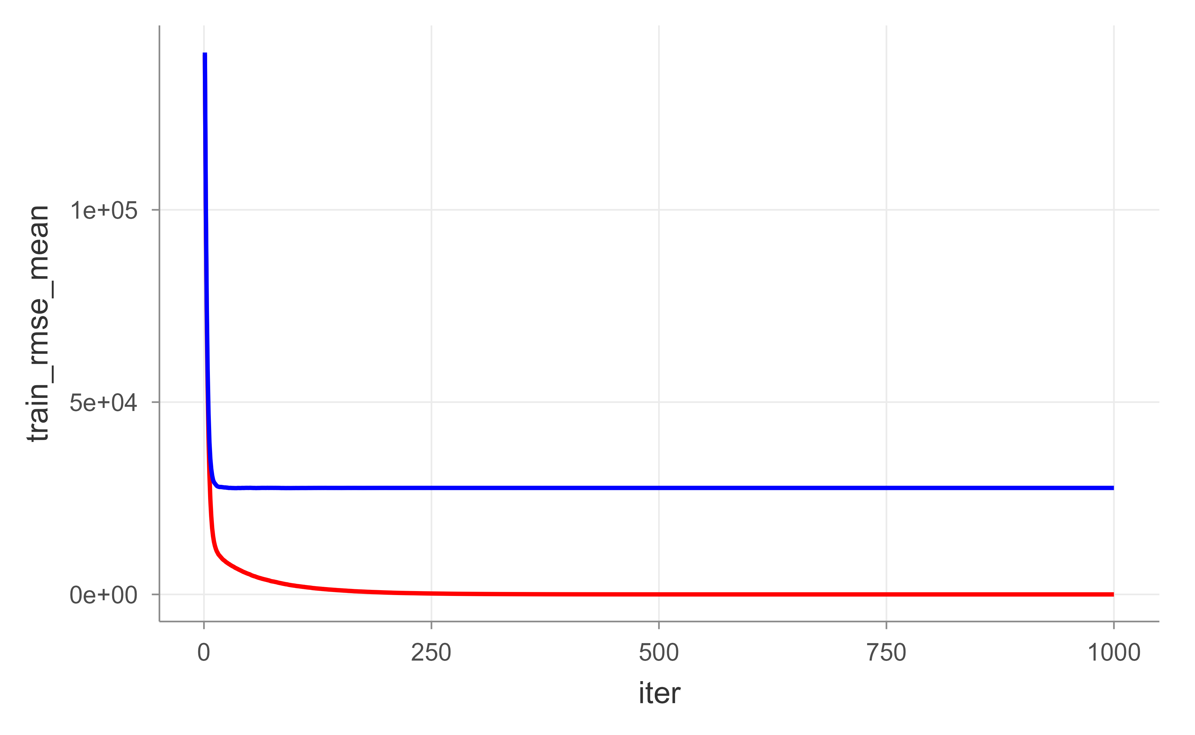
# get number of trees that minimize errorxgb.fit1$evaluation_log%>%dplyr::summarise( ntrees.train =which(train_rmse_mean==min(train_rmse_mean))[1], rmse.train =min(train_rmse_mean), ntrees.test =which(test_rmse_mean==min(test_rmse_mean))[1], rmse.test =min(test_rmse_mean),)#> ntrees.train rmse.train ntrees.test rmse.test#> 1 976 0.05134272 34 27635.11## ntrees.train rmse.train ntrees.test rmse.test## 1 965 0.5022836 60 27572.31# plot error vs number treesggplot(xgb.fit1$evaluation_log)+geom_line(aes(iter, train_rmse_mean), color ="red")+geom_line(aes(iter, test_rmse_mean), color ="blue")
Figure 11.9: Training (red) and cross-validated test (blue) RMSE by boosting round for the default XGBoost fit, illustrating overfitting as the number of trees grows.
In Figure 11.9, the red (training) curve keeps falling while the blue (test) curve flattens and then turns up: a textbook picture of overfitting as trees accumulate. Rather than guessing the right number of rounds, we can let XGBoost stop on its own once the test error stops improving, using early_stopping_rounds. Figure 11.10 shows the result.
Show code
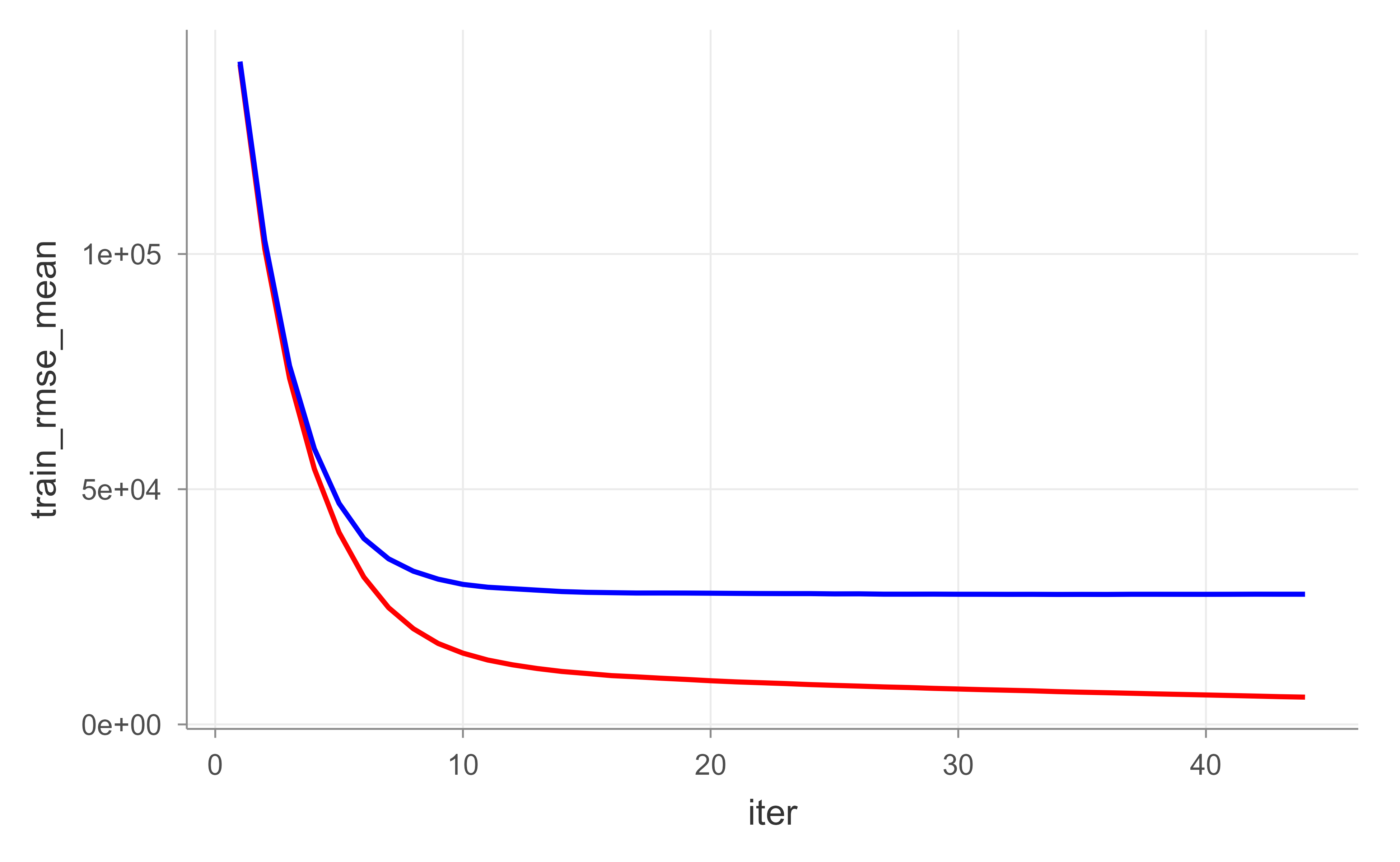
# reproducibilityset.seed(123)xgb.fit2<-xgb.cv( data =features_train, label =response_train, nrounds =1000, nfold =5, objective ="reg:squarederror", # for regression models verbose =0, # silent, early_stopping_rounds =10# stop if no improvement for 10 consecutive trees)# plot error vs number treesggplot(xgb.fit2$evaluation_log)+geom_line(aes(iter, train_rmse_mean), color ="red")+geom_line(aes(iter, test_rmse_mean), color ="blue")
Figure 11.10: Training (red) and cross-validated test (blue) RMSE by boosting round when XGBoost uses early stopping, which halts training once the test error stops improving.
11.10.2.1 Tuning
XGBoost has its own set of tuning parameters, which map onto the general boosting knobs from earlier:
eta: learning rate.
max_depth: tree depth.
min_child_weight: minimum number of observations in each terminal node.
subsample: fraction of training rows sampled for each tree.
colsample_bytrees: fraction of columns sampled for each tree.
We can bundle these into a params list and pass it to xgb.cv().
As with gbm, the systematic approach is a grid search over these parameters.
Show code
# create hyperparameter gridhyper_grid<-expand.grid( eta =c(.01, .05, .1, .3), max_depth =c(1, 3, 5, 7), min_child_weight =c(1, 3, 5, 7), subsample =c(.65, .8, 1), colsample_bytree =c(.8, .9, 1), optimal_trees =0, # a place to dump results min_RMSE =0# a place to dump results)nrow(hyper_grid)#> [1] 576
Warning
This grid has hundreds of combinations, and a full search over it can take roughly six hours. The loop below is therefore set to eval = FALSE. In practice, start with a coarse grid and refine.
Show code
# grid searchfor(iin1:nrow(hyper_grid)){# create parameter listparams<-list( eta =hyper_grid$eta[i], max_depth =hyper_grid$max_depth[i], min_child_weight =hyper_grid$min_child_weight[i], subsample =hyper_grid$subsample[i], colsample_bytree =hyper_grid$colsample_bytree[i])# reproducibilityset.seed(123)# train modelxgb.tune<-xgb.cv( params =params, data =features_train, label =response_train, nrounds =5000, nfold =5, objective ="reg:squarederror", # for regression models verbose =0, # silent, early_stopping_rounds =10# stop if no improvement for 10 consecutive trees)# add min training error and trees to gridhyper_grid$optimal_trees[i]<-which.min(xgb.tune$evaluation_log$test_rmse_mean)hyper_grid$min_RMSE[i]<-min(xgb.tune$evaluation_log$test_rmse_mean)}hyper_grid%>%dplyr::arrange(min_RMSE)%>%head(10)
Once the search points to good values, we train the final model with xgboost() (the non-cross-validated fitting function) on the full training data.
Show code
# parameter listparams<-list( eta =0.01, max_depth =5, min_child_weight =5, subsample =0.65, colsample_bytree =1)# train final modelxgb.fit.final<-xgboost( params =params, data =features_train, label =response_train, nrounds =1576, objective ="reg:squarederror", verbose =0)
11.10.2.2 Visualization
The same interpretation tools we used for gbm apply here, with XGBoost-specific functions.
11.10.2.2.1 Variable Importance
XGBoost reports three importance measures, each answering a slightly different question:
Gain: the relative contribution of a feature to the model (this is the analogue of gbm::relative.influence).
Cover: the relative number of observations associated with a feature.
Frequency: how often a feature is used to split, as a percentage.
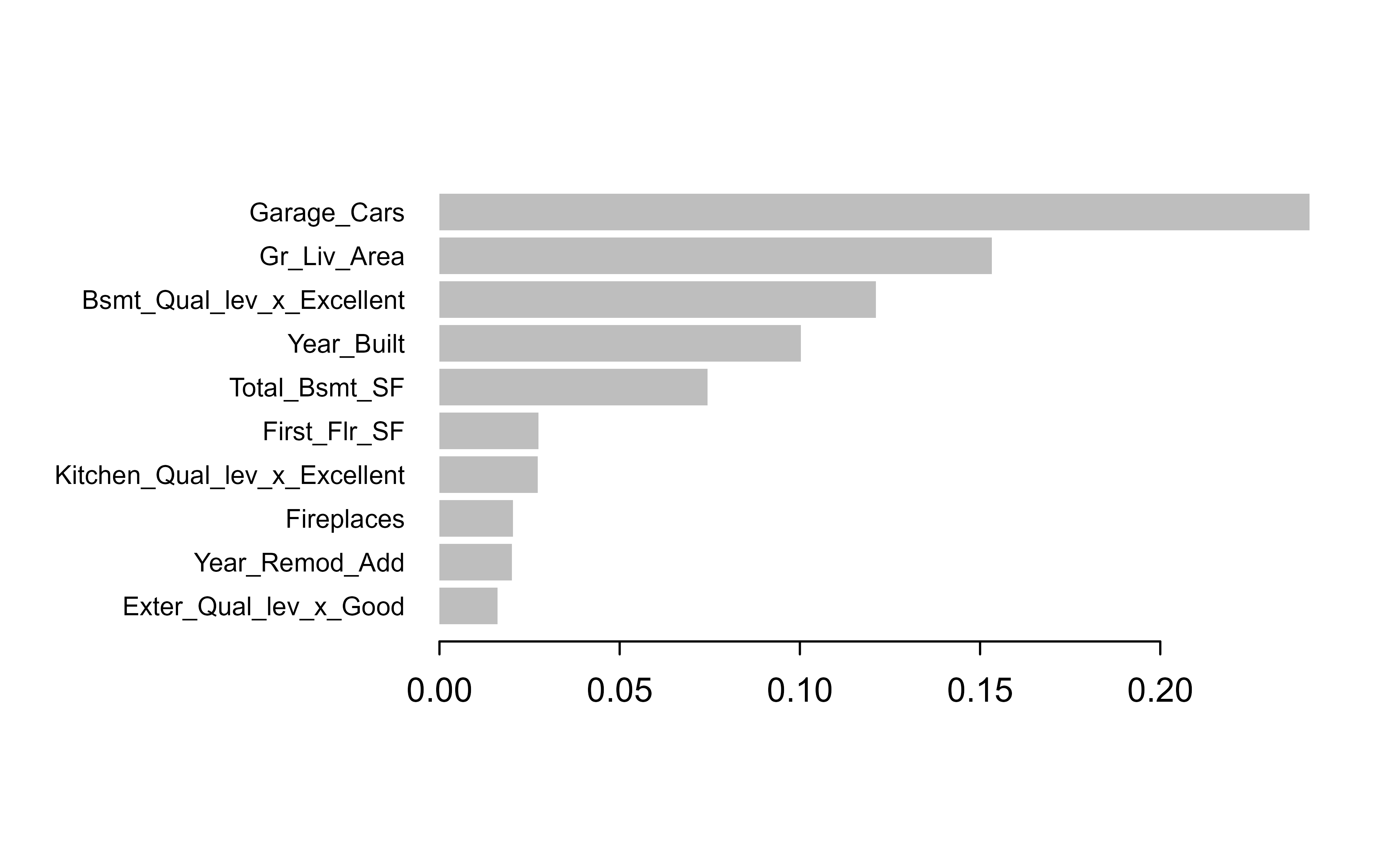
Gain is usually the most informative, so Figure 11.11 plots the top ten features by gain.
Figure 11.11: Top ten features by gain for the final XGBoost model on the Ames housing data.
11.10.2.2.2 Partial dependence plots
PDPs and ICE curves work for XGBoost too, using the one-hot encoded feature names. This chunk is set to eval = FALSE simply to keep the build time down; the code is correct and can be run locally.
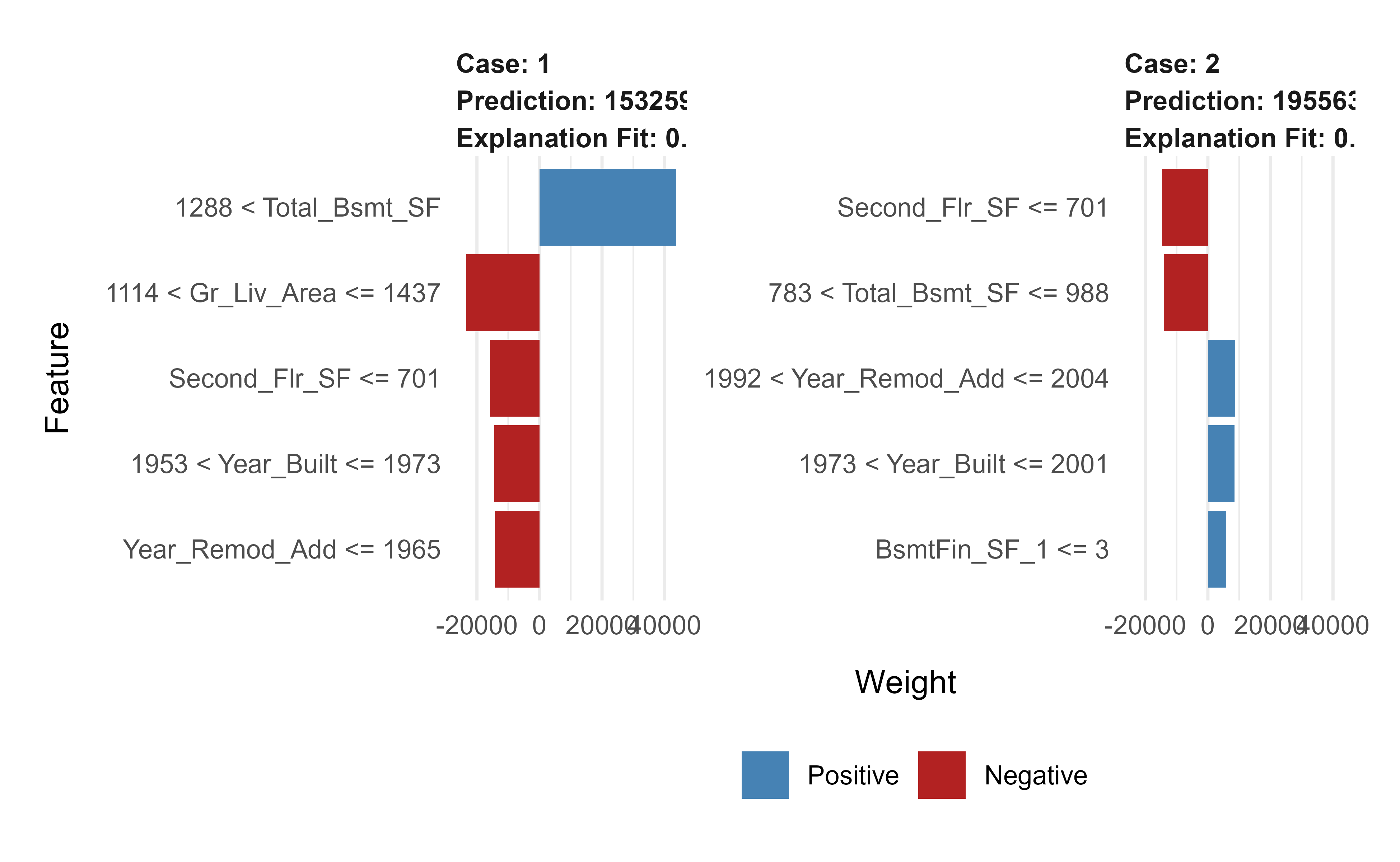
Local explanations work the same way, except the observations must be one-hot encoded with the same treatment plan before they are explained. Figure 11.12 shows the resulting explanations.
Show code
# one-hot encode the local observations to be assessed.local_obs_onehot<-vtreat::prepare(treatplan, local_obs, varRestriction =new_vars)# apply LIMEexplainer<-lime::lime(data.frame(features_train), xgb.fit.final)explanation<-lime::explain(local_obs_onehot, explainer, n_features =5)plot_features(explanation)
Figure 11.12: LIME local explanations for two test observations under the final XGBoost model, using the one-hot encoded features.
11.10.2.3 Prediction
And the final test-set evaluation:
Show code
# predict values for test datapred<-predict(xgb.fit.final, features_test)# resultscaret::RMSE(pred, response_test)#> [1] 22486.75## [1] 21319.3
11.10.3h2o
The h2o package is a Java-based platform aimed at scaling gradient boosting to large data and distributed compute. Its notable features are:
distributed and parallelized computation,
automatic early stopping,
stochastic gradient boosting with column and row sampling,
support for exponential families and many loss functions,
grid search,
the ability to scale to any dataset size (because it is data-distributed),
histogram approximations of continuous variables,
dynamic binning, and
unlimited factor levels.
Note
Every h2o chunk in this section is set to eval = FALSE. They require a running H2O cluster started by h2o.init() (a separate Java process), which is an external dependency that the book build does not assume. The code is correct and idiomatic; start the cluster locally with h2o.init() to run it. The ## lines show representative output from a prior run.
Then convert the data to an H2O frame and fit a baseline GBM with cross-validation.
Show code
# create feature namesy<-"Sale_Price"x<-setdiff(names(ames_train), y)# turn training set into h2o objecttrain.h2o<-as.h2o(ames_train)# training basic GBM model with defaultsh2o.fit1<-h2o.gbm( x =x, y =y, training_frame =train.h2o, nfolds =5)# assess model resultsh2o.fit1
A second fit turns on early stopping with a generous tree budget, so the algorithm decides how many trees it actually needs.
Show code
# training basic GBM model with defaultsh2o.fit2<-h2o.gbm( x =x, y =y, training_frame =train.h2o, nfolds =5, ntrees =5000, stopping_rounds =10, stopping_tolerance =0, seed =123)# model stopped after xx treesh2o.fit2@parameters$ntrees## [1] 3828# cross validated RMSEh2o.rmse(h2o.fit2, xval =TRUE)## [1] 24684.09
11.10.3.1 Tuning
For the full list of parameters, see the H2O.ai GBM tuning guide10. The main parameters group naturally into three families:
Tree complexity:
ntrees: number of trees to train,
max_depth: depth of each tree,
min_rows: minimum observations per terminal node.
Learning rate:
learn_rate: rate at which to descend the loss gradient,
learn_rate_annealing: start with a high learn_rate, then gradually reduce it as trees are added.
Stochasticity:
sample_rate: row sample rate per tree,
col_sample_rate: column sample rate per tree.
H2O gives you two grid-search strategies. The first is a full (Cartesian) grid search over every combination.
Show code
# about 90 mins# create training & validation setssplit<-h2o.splitFrame(train.h2o, ratios =0.75)train<-split[[1]]valid<-split[[2]]# create hyperparameter gridhyper_grid<-list( max_depth =c(1, 3, 5), min_rows =c(1, 5, 10), learn_rate =c(0.01, 0.05, 0.1), learn_rate_annealing =c(.99, 1), sample_rate =c(.5, .75, 1), col_sample_rate =c(.8, .9, 1))# perform grid searchgrid<-h2o.grid( algorithm ="gbm", grid_id ="gbm_grid1", x =x, y =y, training_frame =train, validation_frame =valid, hyper_params =hyper_grid, ntrees =5000, stopping_rounds =10, stopping_tolerance =0, seed =123)# collect the results and sort by our model performance metric of choicegrid_perf<-h2o.getGrid( grid_id ="gbm_grid1", sort_by ="mse", decreasing =FALSE)grid_perf
From the grid we pull the best model and check its validation performance.
Show code
# Grab the model_id for the top model, chosen by validation errorbest_model_id<-grid_perf@model_ids[[1]]best_model<-h2o.getModel(best_model_id)# Now let's get performance metrics on the best modelh2o.performance(model =best_model, valid =TRUE)## H2ORegressionMetrics: gbm## ** Reported on validation data. **#### MSE: 362098307## RMSE: 19028.88## MAE: 12427.99## RMSLE: 0.1403692## Mean Residual Deviance : 362098307
The second strategy is a random discrete grid search. Because the number of combinations explodes as you add hyperparameters, sampling combinations at random (rather than trying them all) finds a good-enough model far faster, even if not the absolute best one.
Show code
# random grid search criteriasearch_criteria<-list( strategy ="RandomDiscrete", stopping_metric ="mse", stopping_tolerance =0.005, stopping_rounds =10, max_runtime_secs =60*60)# perform grid searchgrid<-h2o.grid( algorithm ="gbm", grid_id ="gbm_grid2", x =x, y =y, training_frame =train, validation_frame =valid, hyper_params =hyper_grid, search_criteria =search_criteria, # add search criteria ntrees =5000, stopping_rounds =10, stopping_tolerance =0, seed =123)# collect the results and sort by our model performance metric of choicegrid_perf<-h2o.getGrid( grid_id ="gbm_grid2", sort_by ="mse", decreasing =FALSE)grid_perf
Again we extract and evaluate the top model.
Show code
# Grab the model_id for the top model, chosen by validation errorbest_model_id<-grid_perf@model_ids[[1]]best_model<-h2o.getModel(best_model_id)# Now let's get performance metrics on the best modelh2o.performance(model =best_model, valid =TRUE)## H2ORegressionMetrics: gbm## ** Reported on validation data. **#### MSE: 515072025## RMSE: 22695.2## MAE: 13841.13## RMSLE: 0.1427291## Mean Residual Deviance : 515072025
With the preferred settings chosen, we retrain a final model on the full training data.
Show code
# train final modelh2o.final<-h2o.gbm( x =x, y =y, training_frame =train.h2o, nfolds =5, ntrees =10000, learn_rate =0.01, learn_rate_annealing =1, max_depth =3, min_rows =10, sample_rate =0.75, col_sample_rate =1, stopping_rounds =10, stopping_tolerance =0, seed =123)# model stopped after xx treesh2o.final@parameters$ntrees## [1] 9385# cross validated RMSEh2o.rmse(h2o.final, xval =TRUE)## [1] 23218.45
11.10.3.2 Visualization
H2O provides its own interpretation functions, mirroring what we did with gbm and xgboost.
11.10.3.2.1 Variable Importance
Show code
h2o.varimp_plot(h2o.final, num_of_features =10)
11.10.3.2.2 Partial dependence plots
We can build PDP and ICE plots with the pdp package by supplying a small prediction wrapper that converts H2O output back to a vector.
h2o.partialPlot(h2o.final, data =train.h2o, cols ="Overall_Qual")
One practical difference: h2o’s native function draws categorical levels alphabetically, whereas pdp respects the factor’s level order, which usually makes the plot easier to interpret.
# convert test set to h2o objecttest.h2o<-as.h2o(ames_test)# evaluate performance on new datah2o.performance(model =h2o.final, newdata =test.h2o)## H2ORegressionMetrics: gbm#### MSE: 407532539## RMSE: 20187.44## MAE: 12683.01## RMSLE: 0.100829## Mean Residual Deviance : 407532539# predict with h2o.predicth2o.predict(h2o.final, newdata =test.h2o)## predict## 1 130114.9## 2 162136.7## 3 263438.5## 4 484853.0## 5 219152.9## 6 208616.2#### [879 rows x 1 column]# predict values with predictpredict(h2o.final, test.h2o)
11.11 Partial Dependence Plots
We have used partial dependence plots throughout the chapter; this section gives the formal definition behind them. PDPs are one of the main ways to interpret parameter effects from tree-based models (for example bagging and boosting).
The setup: consider a subvector \(X_S\) of \(l < p\) of the input predictor space \(X\), indexed by \(S \subset \{ 1, \dots, p \}\). Let \(C\) be its complement, so that \(S \cup C = \{1, \dots, p \}\). Writing \(f(X) = f(X_S, X_C)\), the partial dependence of \(f(X)\) on the variables of interest \(X_S\) is defined as the average over the other variables:
\[
f_S(X_S) = E_{X_C} f(X_S, X_C)
\]
which is the marginal average of \(f\). This is a useful description of the effect of the chosen subset on \(f(X)\) as long as the elements of \(X_S\) do not interact strongly with the elements of \(X_C\).
In practice we estimate this expectation by plugging in the observed values of the other variables and averaging:
where \(\{ x_{1C}, \dots, x_{nC}\}\) are the values of \(X_C\) in the training data.
A few points about interpreting this estimate:
Computing it can be expensive in general, but for decision trees \(\bar{f}_S(X_S)\) can be computed efficiently directly from the tree structure.
A PDP represents the effect of \(X_S\) on \(f(X)\)after accounting for the average effects of the other variables \(X_C\).
You cannot read it as the effect of \(X_S\) on \(f(X)\) while ignoring\(X_C\), unless \(X_S\) and \(X_C\) are independent (\(X_S \perp X_C\)).
Warning
PDPs can mislead when the variable of interest is correlated with, or interacts with, the variables being averaged out. ICE curves and accumulated local effects (ALE) plots are useful complements when that is a concern.
To make this concrete, Figure 11.13 and Figure 11.14 show the PDPs for the two most important variables from our gbm Boston model, giving each variable’s marginal effect on the response after integrating out the others.
Show code
plot(boost.boston, i ="rm")# median house prices increase with rm
Figure 11.13: Partial dependence of predicted median house value on the average number of rooms (rm) for the gbm Boston model.
Show code
plot(boost.boston, i ="lstat")# median house prices decrease with lstat
Figure 11.14: Partial dependence of predicted median house value on the percentage of lower-status population (lstat) for the gbm Boston model.
The plots in Figure 11.13 and Figure 11.14 confirm the expected directions: predicted median house price rises with the average number of rooms (rm) and falls as the percentage of lower-status population (lstat) increases.
That analysis used the default shrinkage of \(\lambda = 0.001\). Shrinkage is a tuning parameter, so it is worth trying a different value; here we use a faster learning rate of \(\lambda = 0.2\).
In this case the larger shrinkage (faster learning) gives a lower test MSE, a reminder that the best learning rate is data-dependent and worth tuning rather than assuming.
11.12 Takeaways
A few ideas are worth carrying out of this chapter:
Boosting builds models sequentially, each correcting the errors of the ensemble so far, in contrast to the independent, averaged trees of bagging and random forests.
“Learning slowly” with a small learning rate and many trees is the central design choice; the learning rate \(\lambda\) and the number of trees \(B\) trade off against each other.
AdaBoost reweights misclassified points; gradient boosting generalizes this to fit each new tree to the negative gradient of any differentiable loss, which is why it handles regression, classification, and ranking alike.
In practice you will reach for xgboost, lightgbm, or h2o, which add regularization, early stopping, subsampling, and scalable computation on top of the basic algorithm.
A boosted model is not a black box: variable importance, partial dependence and ICE plots, and LIME together let you explain both the global behavior of the model and individual predictions.
Freund, Yoav, and Robert E Schapire. 1997. “A Decision-Theoretic Generalization of On-Line Learning and an Application to Boosting.”Journal of Computer and System Sciences 55 (1): 119–39. https://doi.org/10.1006/jcss.1997.1504.
Machado, Marcos Roberto, Salma Karray, and Ivaldo Tributino de Sousa. 2019. “LightGBM: An Effective Decision Tree Gradient Boosting Method to Predict Customer Loyalty in the Finance Industry.”2019 14th International Conference on Computer Science and Education (ICCSE), August. https://doi.org/10.1109/iccse.2019.8845529.
Gradient boosted trees routinely win tabular-data competitions and serve as strong baselines in industry precisely because they require little preprocessing and tune to high accuracy.↩︎
Freezing the earlier terms is what keeps the problem cheap and what makes boosting “greedy.” It is also why boosting is robust: no single step can undo the accumulated progress.↩︎
# Boosting {#sec-boosting}```{r}#| include: falsesource("_common.R")```Imagine you are trying to predict house prices and your first model is a small, blunt decision tree (@sec-regression-trees). It captures the broad pattern (bigger houses cost more) but it misses many details, and its errors are large for certain neighborhoods. A natural human reaction would be to look at where the model went wrong and build a second, focused model that specializes in fixing those mistakes, then a third that fixes what is still wrong, and so on. Boosting is exactly this idea made precise: it builds a sequence of simple models, each one trained to correct the errors left behind by the models before it.This stands in contrast to bagging and random forests (@sec-random-forest), where many trees are grown *independently* on bootstrap samples and then averaged. Boosting grows trees *sequentially*: each new tree depends strongly on the trees already built, because it is fit to what they got wrong. There are no bootstrap samples in classic boosting; instead, we repeatedly fit small trees to the *residuals* (the leftover error), not to the original response $Y$ directly.The phrase you will hear in the literature is that boosting "learns slowly." Rather than fitting one large tree that tries to capture everything at once (sometimes called "fitting the data hard"), boosting nudges the model in the right direction a little at a time, scaling each new tree by a small shrinkage factor $\lambda$. Learning slowly turns out to be a feature, not a bug: it concentrates effort on the parts of the problem that are still poorly fit and it guards against overfitting.In this chapter you will build up boosting from its conceptual core to its modern, production-grade implementations. We start with the intuition (gradient descent and slow learning), then give the precise algorithms for regression and classification, work through the original AdaBoost, generalize to gradient boosting, and finish with the libraries you will actually use in practice (`gbm`, `xgboost`, `lightgbm`, and `h2o`), along with the interpretation tools (variable importance, partial dependence, and LIME) that make a boosted model explainable.::: {.callout-important title="Key idea"}Boosting combines many "weak" learners (models that are only slightly better than guessing) into one strong "committee," by training each new learner to fix the mistakes of the current ensemble.:::A few facts worth keeping in mind from the start. Boosting was originally designed for classification (the classic algorithm is AdaBoost.M1 [@freund1997b], and it is sometimes called hypothesis boosting), but it extends naturally to regression. It is widely regarded as one of the best off-the-shelf predictors available.^[Gradient boosted trees routinely win tabular-data competitions and serve as strong baselines in industry precisely because they require little preprocessing and tune to high accuracy.]When should you reach for boosting, and what are the tradeoffs? The following lists summarize the practical case.Boosting tends to offer:- Good predictive accuracy, often state of the art on tabular data.- Several hyperparameters to tune, which gives you a lot of flexibility.- Little need for preprocessing.- Built-in handling of missing data in many implementations (no imputation needed).The costs to weigh against those benefits are:- Because it relentlessly drives down training error, a gradient boosting machine (GBM) can overemphasize outliers and overfit. Cross-validation (@sec-intro) is the main defense.- It can be computationally expensive, especially during a large grid search over hyperparameters.Underneath all of this, the general framework of boosting is a stagewise additive model built from $B$ regression trees, which connects it directly to the additive models of @sec-gam:$$f(x) = \sum_{b=1}^B f^b (x)$$The rest of the chapter unpacks how those component functions $f^b$ are chosen and combined.## Gradient DescentBefore the algorithms, it helps to name the engine that drives modern boosting: gradient descent. Gradient descent is a general recipe for minimizing a function by repeatedly taking a small step in the direction that decreases it fastest (the negative gradient). Gradient boosting is, quite literally, gradient descent applied in "function space," where each step is a new tree.The reasons this framing matters:- Gradient boosting can be generalized to minimize many different loss functions (for example mean squared error or mean absolute error), not just one.- The core idea is to tweak the model iteratively to minimize a cost function.- It works for any differentiable loss function, which is what lets us swap in losses suited to regression, classification, or ranking.::: {.callout-tip title="Intuition"}If the loss is a hill you want to walk down, the gradient points uphill. Boosting reads off the (negative) gradient at the current model, fits a tree to it, and takes a small downhill step scaled by the learning rate.:::If you would like a careful walk-through of the underlying optimization, you can refer to the first book for [more detail](https://bookdown.org/mike/data_analysis/non-linear-regression.html?q=gradient%20d#steepest-descent).## TuningBoosting gives you several knobs, and getting good performance is largely a matter of setting them sensibly. Here are the main ones, with what each controls:- Number of trees: how many sequential trees to grow.- Depth of trees: how many splits $d$ each tree is allowed (this controls how much interaction between variables a single tree can capture).- Learning rate (shrinkage): smaller values reduce overfitting but require more trees and longer fitting time.- Subsampling: training each tree on a random subset of the data adds randomness that can reduce overfitting; tune it with cross-validation (@sec-intro).We will see these same parameters reappear under slightly different names in every library later in the chapter.## Regression BoostingWith the intuition in place, here is the precise algorithm for boosting regression trees. Read it as "start from nothing, then repeatedly fit a small tree to the current residuals and add a shrunken version of it back in."1. Set $\hat{f}(x) = 0$ and $r_i = y_i \forall i$ (in the training set)2. For $b = 1, \dots, B$ repeat 1. Fit a tree $\hat{f}^b$ with $d$ splits ($d + 1$ terminal nodes) to the training data $(X,r)$ 2. Update $\hat{f}$ by adding in a shrunken version of the new tree $\hat{f}(x) \leftarrow \hat{f}(x) + \lambda \hat{f}^b (x)$ 3. Update the residuals $r_i \leftarrow r_i - \lambda \hat{f}^b (x_i)$3. Final boosted model $\hat{f}(x) = \sum_{b=1}^B \lambda \hat{f}^b (x)$<br>Notice how step 2.3 makes the algorithm self-correcting: after each tree is added, the residuals shrink in the regions that tree explained well, so the next tree is automatically drawn to whatever is still poorly fit.This algorithm has three tuning parameters, and understanding how they interact is most of what you need to use boosting well:1. $B$: the number of trees. Boosting *can* overfit if $B$ is too large, so we use cross-validation (@sec-intro) to select $B$.2. $\lambda$: the shrinkage parameter, which controls the rate at which boosting learns. Typical values are 0.01 or 0.001 (the best choice depends on the data at hand). The smaller the $\lambda$, the larger $B$ must be to achieve good performance.3. $d$: the number of splits in each tree. Surprisingly, $d = 1$ often works well, in which case we call the tree a "stump." With $d = 1$, the boosted ensemble is fitting an additive model, since each term involves only one variable. More generally, $d$ is the interaction depth and controls the interaction order of the boosted model (since $d$ splits can involve at most $d$ variables).::: {.callout-note}The inverse relationship between $\lambda$ and $B$ is the single most important thing to internalize. Halving the learning rate roughly doubles the number of trees you need. Slow learners are more accurate but more expensive.:::### Why slow learning regularizes {#sec-boosting-shrinkage-theory}The empirical rule "small $\lambda$, large $B$" has a precise statistical reading. Each boosting iteration adds a basis function $\hat f^b$ aligned with the current negative gradient, and $B$ controls how many such terms enter the model. With $\lambda = 1$ and no constraint, the procedure is greedy least-squares matching pursuit, and the training error can be driven to zero, overfitting. Shrinkage by $\lambda < 1$ damps each step, so that the path traced out by the ensemble as $B$ grows stays close to the path of an L1-penalized (lasso) fit in the space of all trees. In the limit of infinitesimal $\lambda$, increasing $B$ moves the solution along the lasso regularization path with the number of trees playing the role of inverse penalty: more trees correspond to a larger effective model. This is the rigorous content behind the advice to treat $B$ as the regularization parameter to be chosen by cross-validation while fixing $\lambda$ small. It also explains why early stopping (capping $B$ at the cross-validated minimum) is itself a form of regularization, not merely a compute-saving trick.The two parameters trade off through the bias-variance decomposition. Holding $B$ fixed, smaller $\lambda$ means each tree contributes less, raising bias but lowering variance and the risk of fitting noise; the deficit is recovered by raising $B$. Tree depth $d$ controls the complementary axis of complexity: $d = 1$ (stumps) yields a strictly additive model with no interactions (@sec-gam), while depth $d$ permits interactions of order up to $d$. Increasing $d$ lowers bias for genuinely interacting signals but raises variance and the effective number of parameters per tree.### Convergence, consistency, and failure modes {#sec-boosting-theory}A few theoretical facts frame when boosting works and when it does not.- Training-error guarantee for AdaBoost. If every weak learner achieves weighted error $\overline{err}_m = \tfrac{1}{2} - \delta_m$ with edge $\delta_m > 0$, then the training misclassification rate is bounded by $\prod_m \sqrt{1 - 4\delta_m^2} \le \exp(-2\sum_m \delta_m^2)$, which goes to zero exponentially in the number of rounds. This is the original sense in which boosting "turns weak learners into a strong learner."- Margins and resistance to overfitting. AdaBoost often keeps improving test accuracy even after training error reaches zero. The margin explanation is that continued rounds increase the classification margins $y_i f(x_i) / \sum_m |\alpha_m|$, and generalization bounds depend on the margin distribution rather than on the number of rounds, so a larger margin can keep test error falling. This is not a guarantee: with enough noise, boosting does eventually overfit.- Statistical view and consistency. Viewing boosting as stagewise function-space minimization of a convex surrogate loss connects it to nonparametric regression: with appropriately shrunken steps and early stopping, boosting with trees is consistent for the regression function or the Bayes classifier under standard conditions. The estimator is biased toward simpler (low-interaction, shrunken) fits, trading variance for bias in the usual way.- Failure modes. Boosting breaks down or underperforms when (i) labels are noisy or contain outliers and the loss is exponential, since $e^{-yf}$ places enormous weight on grossly misclassified points and the ensemble chases them (use deviance, Huber, or quantile losses instead); (ii) the base learners are too strong (deep trees with $\lambda = 1$), which removes the slow-learning safeguard and overfits in a handful of rounds; (iii) $B$ is left uncross-validated, in which case the relentless drive to reduce training loss eventually fits noise; and (iv) classes are extremely imbalanced, where accuracy-driven reweighting can be dominated by the majority class unless the loss is reweighted.### Computational cost and practical tuning {#sec-boosting-howto}The dominant cost of boosting is growing $B$ trees sequentially, each over $n$ observations and $p$ features. With exact split finding, building one depth-$d$ tree costs $O(d \cdot n p)$ after an initial $O(np \log n)$ feature sort, so the full fit is roughly $O(B \cdot d \cdot n p)$. Two engineering ideas in modern libraries cut this: histogram binning of each feature into $K$ bins reduces split scanning from $O(n)$ to $O(K)$ per feature (LightGBM, and XGBoost's `tree_method = "hist"`), and row/column subsampling shrinks the effective $n$ and $p$ per tree. Sequentiality means the $B$ dimension cannot be parallelized; the parallelism in XGBoost and LightGBM is within each tree (across features and split candidates), which is why they scale with cores rather than with tree count.A workable tuning recipe, consistent with the grid searches later in the chapter, is:1. Fix a small learning rate ($\lambda$ or `eta` around 0.05 to 0.1 for tuning, optionally smaller for the final fit) and choose $B$ by cross-validation or early stopping. Do not tune $\lambda$ and $B$ independently; tune the others at a moderate $\lambda$, then lower $\lambda$ and raise $B$ proportionally for the final model.2. Set tree depth $d$ (`interaction.depth`, `max_depth`) to the interaction order you expect; 3 to 6 is typical for tabular data, $d = 1$ when you want a transparent additive model.3. Add stochasticity (`bag.fraction`, `subsample`, `colsample_bytree` in $[0.5, 0.9]$) as a cheap variance reducer.4. Use the leaf-size and regularization knobs (`min_child_weight`, `n.minobsinnode`, `gamma`, `lambda`, `alpha`) to control overfitting once the above are set.Diagnose by plotting cross-validated loss against the number of trees (as in @fig-boosting-gbm-perf-slow and @fig-boosting-xgb-overfit): a test curve that turns upward signals too many trees or too aggressive a learner.<br>## Classification BoostingBoosting was born in the classification setting, so it is worth seeing the idea there directly. Consider a two-class problem coded so that $Y \in \{ -1, 1\}$, with a vector of predictors $X$.We have a classifier $G(X)$ that predicts either $-1$ or $1$. Its error rate on the training sample is the fraction of misclassified points:$$\bar{err} = \frac{1}{n} \sum_{i=1}^n I(y_i \neq G(x_i))$$A *weak classifier* is one whose error rate is only slightly better than random guessing. The boosting strategy is to sequentially apply a weak classification algorithm, producing a sequence of weak classifiers $G_m(x), m = 1, \dots, M$ (here $M$ plays the role that $B$ did above). Each one is deliberately simple; the power comes from how they are combined.Their predictions are combined through a weighted majority vote to produce the final prediction:$$G(x) = sign (\sum_{m=1}^M \alpha_m G_m (x))$$where the weights $\alpha_m, m = 1, \dots, M$ are computed by the boosting algorithm and give the highest influence to the best classifiers. So a confident, accurate weak learner gets a loud vote, and a barely-better-than-chance one gets a quiet one.The other half of the mechanism is reweighting the *data*. At each boosting step, weights $w_1, \dots, w_n$ are attached to the training observations $(x_i, y_i), i = 1, \dots, n$. To start, the weights are equal, $w_i = \frac{1}{n}$, so there is no preference at the first step.After each iteration, the weights are updated: observations that classifier $G_{m-1}(x)$ got wrong have their weights increased, and those it got right have their weights decreased. As the iterations continue, observations that are hard to classify accumulate ever more influence, so each successive classifier is forced to concentrate on the cases its predecessors kept missing.::: {.callout-tip title="Intuition"}Boosting is like a study group where, after every quiz, you spend more time on the questions the group keeps getting wrong, and you trust the answers of whoever has been most reliable so far.:::<br>### Why boosting works so wellIt is reasonable to ask *why* this procedure should produce such accurate predictors. The cleanest explanation comes from viewing boosting as a basis function expansion (@sec-spline):$$f(x) = \sum_{m=1}^M \beta_m b(x; \gamma_m)$$where- $\beta_m$ are the expansion coefficients- $b(x, \gamma)$ are simple functions of the multivariate inputs $x$ and parameters $\gamma$From this angle, boosting is simply a way of fitting an additive expansion in which the basis functions are the individual classifiers $G_m(x) \in \{ -1, 1\}$.To fit such a model, we would like to minimize some loss function averaged over the training data (for example, squared error loss):$$\min_{\{\beta_m , \gamma_m \}^M_1} \sum_{i=1}^n L (y_i, \sum_{m=1}^M \beta_m b(x_i; \gamma_m))$$For most loss functions $L(y, f(x))$ and basis functions $b(x; \gamma)$, solving this jointly over all $M$ terms at once is computationally intensive. The trick that makes boosting tractable is to instead solve a much easier subproblem: fitting just a single basis function at a time,$$\min_{\{\beta, \gamma\}} \sum_{i=1}^n L(y_i, \beta b (x_i; \gamma))$$We then approximate the full minimization by sequentially adding new basis functions to the expansion without going back to readjust the parameters and coefficients already in place. This procedure is called forward stagewise additive modeling: at each iteration $m$, we solve for the optimal basis function $b(x, \gamma_m)$ and coefficient $\beta_m$ to add to the current expansion $f_{m-1}(x)$, obtaining $f_m(x)$, and we repeat while holding the previously added terms fixed.^[Freezing the earlier terms is what keeps the problem cheap and what makes boosting "greedy." It is also why boosting is robust: no single step can undo the accumulated progress.]A concrete example makes this tangible. With squared error loss,$$L(y, f(x)) = (y - f(x))^2$$the loss of adding one more term becomes$$\begin{aligned}L(y_i, f_{m-1}(x_i) + \beta_m b(x_i; \gamma_m) &= (y_i - f_{m-1}(x_i) - \beta_mb(x_i; \gamma_m))^2 \\&= (r_{im} - \beta_mb(x_i; \gamma_m))^2\end{aligned}$$where $r_{im} = y_i - f_{m-1}(x)$ is the residual of the current model on the $i$-th observation. In words: the next term $\beta_m b(x; \gamma_m)$ is just the one that best fits the current residuals. This is precisely the regression boosting algorithm from the previous section, now derived rather than asserted.<br>## AdaBoostAdaBoost was the first boosting algorithm, and it remains the cleanest example of the reweighting idea in action. Its logic can be stated in three sentences:1. It combines "weak learners" (often stumps) to make classifications.2. Each stump gets a different weight in the final vote.3. Each stump is built sequentially, focused on the previous stump's mistakes.<br>Here is the precise procedure, AdaBoost.M1:1. Initialize the observation weights $w_i = \frac{1}{N}, i = 1, \dots, N$2. For $m = 1$ to M 1. Fit a classifier $G_m(x)$ to the training data with weights $w_i$ 2. Calculate $err_m = \frac{\sum_{i=1}^{N} w_i I(y_i \neq G_m(x_i))}{\sum_{i=1}^N w_i}$ 3. Calculate $\alpha_m = \log (\frac{1 - err_m}{err_m})$ 4. Set $w_i \leftarrow w_i \times \exp(\alpha_m \times I (y_i \neq G_m(x_i))), i = 1, \dots, N$3. $G(x) = sign(\sum_{m=1}^M \alpha_m G_m(x))$Reading the steps together: a low-error classifier earns a large $\alpha_m$ (a loud vote in step 3), and step 2.4 multiplies up the weights of exactly the points it misclassified, so the next round leans into them.It is not obvious at first, but AdaBoost.M1 is equivalent to forward stagewise modeling using the loss function [@hastie2001a, 10.4]$$L(y, f(x)) = \exp(-y f(x))$$which is the "exponential loss." This loss is closely related to the binomial negative log-likelihood (deviance), although the two behave differently with finite, real-world data. The exponential loss is attractive mainly because it makes the computation in step 2 fall out cleanly.### Deriving AdaBoost from exponential loss {#sec-boosting-adaboost-derivation}The claim that AdaBoost.M1 is forward stagewise additive modeling under exponential loss is worth proving, because the proof produces the exact formulas for $\alpha_m$ and the weight update rather than leaving them as recipes. We work with $y \in \{-1, 1\}$ and an additive model $f(x) = \sum_m \alpha_m G_m(x)$ where each $G_m(x) \in \{-1, 1\}$.At stage $m$ the current model is $f_{m-1}(x)$ and we must solve$$(\alpha_m, G_m) = \underset{\alpha, G}{\operatorname{argmin}} \sum_{i=1}^N \exp\!\big(-y_i \, (f_{m-1}(x_i) + \alpha G(x_i))\big).$$Define $w_i^{(m)} = \exp(-y_i f_{m-1}(x_i))$. These weights depend on neither $\alpha$ nor $G$, so they act as fixed observation weights at this stage, and the objective factorizes as$$\sum_{i=1}^N w_i^{(m)} \exp(-\alpha\, y_i G(x_i)).$$ {#eq-boosting-ada-obj}Because $y_i G(x_i) = 1$ when the point is correctly classified and $-1$ when misclassified, we split the sum:$$\begin{aligned}\sum_{i=1}^N w_i^{(m)} \exp(-\alpha\, y_i G(x_i))&= e^{-\alpha} \sum_{y_i = G(x_i)} w_i^{(m)} + e^{\alpha} \sum_{y_i \neq G(x_i)} w_i^{(m)} \\&= (e^{\alpha} - e^{-\alpha}) \sum_{i=1}^N w_i^{(m)} I(y_i \neq G(x_i)) + e^{-\alpha} \sum_{i=1}^N w_i^{(m)}.\end{aligned}$$ {#eq-boosting-ada-split}Now optimize in two steps. For any fixed $\alpha > 0$, only the first term in @eq-boosting-ada-split depends on $G$ (and $e^{\alpha} - e^{-\alpha} > 0$), so the optimal classifier minimizes the weighted error,$$G_m = \underset{G}{\operatorname{argmin}} \sum_{i=1}^N w_i^{(m)} I(y_i \neq G(x_i)),$$which is exactly step 2.1 of the algorithm: fit a classifier to the weighted data. Given $G_m$, write the weighted error as$$\overline{err}_m = \frac{\sum_{i=1}^N w_i^{(m)} I(y_i \neq G_m(x_i))}{\sum_{i=1}^N w_i^{(m)}}.$$Substituting $G_m$ into @eq-boosting-ada-split and dividing by the constant $\sum_i w_i^{(m)}$ leaves the scalar function$$\phi(\alpha) = (e^{\alpha} - e^{-\alpha})\, \overline{err}_m + e^{-\alpha}.$$Setting $\phi'(\alpha) = (e^{\alpha} + e^{-\alpha})\overline{err}_m - e^{-\alpha} = 0$ gives $e^{2\alpha} \overline{err}_m = 1 - \overline{err}_m$, hence$$\alpha_m = \tfrac{1}{2} \log\!\frac{1 - \overline{err}_m}{\overline{err}_m}.$$ {#eq-boosting-ada-alpha}This matches step 2.3 of AdaBoost.M1 up to the factor $\tfrac{1}{2}$; the factor is immaterial because the final classifier is $\operatorname{sign}(\sum_m \alpha_m G_m)$, and scaling every $\alpha_m$ by a common constant leaves the sign unchanged. Finally, the weights for the next stage are $w_i^{(m+1)} = \exp(-y_i f_m(x_i)) = w_i^{(m)} \exp(-\alpha_m y_i G_m(x_i))$. Using $-y_i G_m(x_i) = 2 I(y_i \neq G_m(x_i)) - 1$,$$w_i^{(m+1)} = w_i^{(m)} \exp\!\big(2\alpha_m I(y_i \neq G_m(x_i))\big) \, e^{-\alpha_m}.$$The factor $e^{-\alpha_m}$ is common to all observations and cancels under the renormalization in step 2.2, so the update is equivalent to $w_i \leftarrow w_i \exp(2\alpha_m I(y_i \neq G_m(x_i)))$, which is step 2.4 (again with the harmless factor of two folded into $\alpha_m$). Every line of AdaBoost.M1 has now been derived from the single choice of exponential loss.We can confirm @eq-boosting-ada-alpha numerically: the closed-form $\alpha_m$ should coincide with the value that minimizes the weighted exponential-loss objective @eq-boosting-ada-obj at a single stage.```{r}# verify AdaBoost's alpha minimizes the stage-m exponential lossset.seed(1)n <-200x <-runif(n, -1, 1)y <-ifelse(x +rnorm(n, 0, 0.5) >0, 1L, -1L) # labels in {-1, 1}w <-rep(1/ n, n) # equal stage-1 weightsG <-ifelse(x >0, 1L, -1L) # a stump classifiererr <-sum(w * (y != G)) /sum(w)alpha_closed <-0.5*log((1- err) / err) # eq closed formobj <-function(a) sum(w *exp(-a * y * G)) # stage objectivealpha_numeric <-optimize(obj, interval =c(-5, 5))$minimumc(closed_form = alpha_closed, numeric = alpha_numeric)```The two agree to numerical precision, confirming the derivation.### What exponential loss estimates {#sec-boosting-exploss-population}Stagewise minimization of exponential loss is not arbitrary: its population minimizer is half the log-odds. Minimizing $E_{Y\mid x}[e^{-Y f(x)}]$ pointwise over $f(x)$,$$\frac{\partial}{\partial f(x)} \Big( P(Y=1\mid x)\, e^{-f(x)} + P(Y=-1\mid x)\, e^{f(x)} \Big) = 0,$$gives $-P(Y=1\mid x) e^{-f(x)} + P(Y=-1\mid x) e^{f(x)} = 0$, so$$f^{*}(x) = \tfrac{1}{2} \log \frac{P(Y=1\mid x)}{P(Y=-1\mid x)}.$$ {#eq-boosting-exploss-pop}Thus $\operatorname{sign}(f^{*}(x))$ is the Bayes classifier, which is why driving down exponential loss yields good classification, and inverting @eq-boosting-exploss-pop recovers calibrated probabilities $P(Y=1\mid x) = 1/(1 + e^{-2f^{*}(x)})$. The deviance loss $\log(1 + e^{-2yf(x)})$ has the same population minimizer but grows only linearly (rather than exponentially) in the margin $-yf(x)$, which is precisely why it is more robust to mislabeled points and outliers: a single grossly misclassified observation cannot dominate the sum.::: {.callout-note}Both exponential and deviance losses target the same $f^{*}$, so they agree in the infinite-data limit. They differ in finite samples through how aggressively they penalize large negative margins. This is the rigorous version of the earlier remark that the two "behave differently with finite, real-world data.":::::: {.callout-note}AdaBoost did not start from "let's minimize exponential loss." It was designed first and only later understood as stagewise minimization of that loss. This after-the-fact view is what opened the door to generalizing it.:::There are, of course, many other loss functions. We typically choose one because- it is robust to certain data properties (for example, outliers), or- it makes the computation easier.The key generalization is this: when a loss function is differentiable, we can use its gradient to guide the optimization. That observation is the foundation of gradient boosting (gradient boosting models, "GBM"; formerly known as Multiple Additive Regression Trees, or MART), which is the subject of the next section.<br>## Gradient BoostingGradient boosting generalizes AdaBoost from one special loss to *any* differentiable loss, by replacing "reweight the misclassified points" with "fit the next tree to the negative gradient of the loss." This single change is what makes the method so flexible.A few orienting points before the algorithm:- It is a generalization of [AdaBoost].- The algorithm XGBoost has become one of the standard implementations of gradient boosting and is available in both R and Python. - It uses Newton-Raphson for its optimization (a second-order Taylor approximation of the loss) instead of plain gradient descent. - This improves efficiency in more complicated settings than the original gradient boosting algorithms.- Additional regularization, built-in cross-validation, and handling of missing data are standard features of modern implementations.It helps to contrast gradient boosting with AdaBoost directly. Gradient boosting starts with a single leaf, an initial guess shared by all samples. As in AdaBoost, each new tree is built from the previous trees' errors, and the trees are scaled before being added. But there are two differences: gradient boosting scales every tree by the same amount (the learning rate), and each tree can be larger than a stump.::: {.callout-tip title="Intuition"}Scaling each tree by the learning rate means taking a small, deliberate step in the right direction rather than a giant leap. Many small steps reach a better place than a few large ones.:::<br>### Gradient Boost RegressionHere is the regression algorithm written out. The structure mirrors the regression boosting algorithm from before, but step 2.1 now computes a *pseudo-residual* from the gradient of the loss, which is what lets us use losses other than squared error.Input: Data $\{(x_i, y_i)\}^n_{i=1}$ and a differentiable Loss Function $L(y_i, F(x))$ (e.g., Regression: squared residual: $0.5(\text{Observed} - \text{Predicted})^2$ )Step 1: Initialize model with a constant value: $F_0(x) = \underset{\gamma}{\operatorname{argmin}} \sum_{i=1}^n L(y_i, \gamma)$Step 2: for $m = 1 \to M$ (number of trees):1. Compute the (pseudo) residual: $r_{im} = - [ \frac{\partial L( y_i, F(x_i))}{\partial F(x_i)}]_{F(x) = F_{m-1}(x)}$ for $i = 1, \dots, n$ (where $\frac{\partial L( y_i, F(x_i))}{\partial F(x_i)}$ is the gradient, ergo the name gradient boost)2. Fit a regression tree to the $r_{im}$ values and create terminal regions $R_{jm}$ for $j = 1, \dots, J_m$3. For $j = 1, \dots, J_m$ compute $\gamma_{jm} = \underset{\gamma}{\operatorname{argmin}} \sum_{x_i \in R_{ij}} L(y_i, F_{m-1}(x_i) + \gamma)$4. Update $F_m (x) = F_{m-1}(x) + \nu \sum_{j=1}^{J_m} \gamma_{jm} I(x \in R_{jm})$ where $\nu$ is the learning rate (0 to 1) (smaller value means slower learning rate)Output: $F_M(x)$For squared error loss, the pseudo-residual in step 2.1 reduces exactly to the ordinary residual $y_i - F_{m-1}(x_i)$, which is why the earlier regression algorithm is a special case of this one.#### Why fit the tree to the negative gradient {#sec-boosting-functional-gd}The algorithm above is gradient descent performed in function space, and seeing this explicitly explains both the pseudo-residual and the separate leaf-fitting step. Regard the training loss$$\mathcal{L}(F) = \sum_{i=1}^n L(y_i, F(x_i))$$as a function of the $n$-vector of fitted values $\mathbf{F} = (F(x_1), \dots, F(x_n))$. Ordinary steepest descent would take the step $\mathbf{F}_m = \mathbf{F}_{m-1} - \nu\, \mathbf{g}_m$ where $\mathbf{g}_m$ is the gradient with components$$g_{im} = \left[\frac{\partial L(y_i, F(x_i))}{\partial F(x_i)}\right]_{F = F_{m-1}},$$so $-g_{im}$ is precisely the pseudo-residual $r_{im}$ of step 2.1. The difficulty is that $-\mathbf{g}_m$ is defined only at the $n$ training points; to obtain a function we can evaluate at new $x$, we fit a regression tree to the $n$ pairs $(x_i, r_{im})$. That tree is the closest representable function (in least-squares projection) to the unconstrained steepest-descent direction,$$\hat{f}^m = \underset{f \in \mathcal{T}}{\operatorname{argmin}} \sum_{i=1}^n \big(r_{im} - f(x_i)\big)^2,$$ {#eq-boosting-gb-projection}where $\mathcal{T}$ is the class of depth-$d$ trees. This is why the tree in step 2.2 is always fit by squared error to the residuals, even when the model loss $L$ is something else entirely: the squared-error fit is the projection of the gradient onto the tree class.#### Deriving the optimal leaf values {#sec-boosting-leaf-values}Once the tree has fixed the partition $\{R_{jm}\}$, the leaf values $\gamma_{jm}$ are chosen by a separate one-dimensional optimization (step 2.3) rather than reused from the gradient. The reason is that the gradient gives the right *direction* but not the optimal *step size* within each region. For squared error, $L(y, F) = \tfrac{1}{2}(y - F)^2$, the leaf optimization$$\gamma_{jm} = \underset{\gamma}{\operatorname{argmin}} \sum_{x_i \in R_{jm}} \tfrac{1}{2}\big(y_i - F_{m-1}(x_i) - \gamma\big)^2$$has the closed form $\gamma_{jm} = \operatorname{mean}_{x_i \in R_{jm}}(y_i - F_{m-1}(x_i))$, the average residual in the leaf, confirming again that the Gaussian case reduces to the plain regression boosting algorithm.For a general loss, expand the leaf objective $\Phi_j(\gamma) = \sum_{x_i \in R_{jm}} L(y_i, F_{m-1}(x_i) + \gamma)$ to second order around $\gamma = 0$:$$\Phi_j(\gamma) \approx \Phi_j(0) + \gamma \sum_{x_i \in R_{jm}} g_{im} + \tfrac{1}{2} \gamma^2 \sum_{x_i \in R_{jm}} h_{im},\qquad h_{im} = \left[\frac{\partial^2 L(y_i, F(x_i))}{\partial F(x_i)^2}\right]_{F = F_{m-1}}.$$Minimizing this quadratic gives the Newton leaf value$$\gamma_{jm} = -\frac{\sum_{x_i \in R_{jm}} g_{im}}{\sum_{x_i \in R_{jm}} h_{im}}.$$ {#eq-boosting-newton-leaf}This single formula is the engine behind both the binary classification closed form quoted in the next section and the XGBoost objective derived later.::: {.callout-note}Gradient boosting separates the two questions "which way?" and "how far?": the tree structure is found by least-squares fitting to the negative gradient (the direction), while the leaf values are found by exactly minimizing the true loss within each region (the step). Conflating the two by reusing the gradient as the leaf value would be valid only for squared error.:::<br>Let us see it in action. The `gbm` package fits gradient boosted models in R. We will start with the familiar `Boston` housing data, predicting median home value (`medv`) from the other variables. The `distribution = "gaussian"` argument selects squared error loss for this regression problem.```{r fig-boosting-boston-relinf, message=FALSE, warning=FALSE, fig.cap="Relative influence of each predictor in the gbm boosted model for the Boston housing data, ranked from most to least important."}library(gbm)library(ISLR2)library(tree)set.seed(1)train <-sample(1:nrow(Boston), nrow(Boston)/2)boston.test <- Boston[-train, "medv"]boost.boston <-gbm( medv ~ .,data = Boston[train, ],distribution ="gaussian", # because this is regression setting# distribution = "bernoulli", # use this for classificationn.trees =5000, # number of treesinteraction.depth =4# limits the depth of each tree )summary(boost.boston) #rm and lstate are most important```The `summary()` output ranks the variables by relative influence, shown in @fig-boosting-boston-relinf. Here `rm` (average number of rooms) and `lstat` (percent lower-status population) dominate, which matches the intuition that house size and neighborhood drive price.For a fuller workflow (tuning, visualization, and prediction), we follow an example by the University of Cincinnati^[<http://uc-r.github.io/gbm_regression>], using the larger Ames housing data set. First, we load the packages that support the workflow.```{r}library(rsample) # data splittinglibrary(gbm) # basic implementationlibrary(xgboost) # a faster implementation of gbmlibrary(caret) # an aggregator package for performing many machine learning modelslibrary(h2o) # a java-based platformlibrary(pdp) # model visualizationlibrary(ggplot2) # model visualizationlibrary(lime) # model visualizationlibrary(AmesHousing)```It is worth knowing the personality of the `gbm` implementation before we lean on it. The `gbm` package:- can handle up to 1024 factor levels,- supports many loss functions,- has no automated early stopping, and- offers internal cross-validation that can be combined with parallelization.We split the Ames data into training (70%) and test (30%) sets, using a fixed seed so the results are reproducible.```{r}# Create training (70%) and test (30%) sets for the AmesHousing::make_ames() data.# Use set.seed for reproducibilityset.seed(123)ames_split <-initial_split(AmesHousing::make_ames(), prop = .7)ames_train <-training(ames_split)ames_test <-testing(ames_split)```Now we fit a first model. Note the deliberately slow learning rate (`shrinkage = 0.001`) paired with a large number of trees (`n.trees = 10000`) and shallow stumps (`interaction.depth = 1`). The `cv.folds = 5` argument turns on 5-fold cross-validation so we can read off how many trees we actually need.```{r}# for reproducibilityset.seed(123)# train GBM modelgbm.fit <-gbm(formula = Sale_Price ~ .,distribution ="gaussian",data = ames_train,n.trees =10000,interaction.depth =1,shrinkage =0.001,cv.folds =5,n.cores =NULL, # will use all cores by defaultverbose =FALSE )# print resultsprint(gbm.fit)```The cross-validation error tells us the best number of trees and, taking its square root, the cross-validated RMSE in dollars.```{r fig-boosting-gbm-perf-slow, fig.cap="Cross-validated loss as a function of the number of trees for the slow-learning gbm fit on the Ames data, with the optimal number of trees marked by the dashed line."}# get MSE and compute RMSEsqrt(min(gbm.fit$cv.error))## [1] 29133.33# plot loss function as a result of n trees added to the ensemblegbm.perf(gbm.fit, method ="cv")```@fig-boosting-gbm-perf-slow shows the loss falling as trees are added, with the optimal point marked. Because the learning rate is so small, the curve is still descending after many thousands of trees: a small learning rate can demand a great many trees.#### TuningSince a tiny learning rate forces a huge tree count, the natural next move is to trade some of that slowness for speed: raise the learning rate (which lets us use fewer trees) and let each tree be a little deeper. The following model uses `shrinkage = 0.1` and `interaction.depth = 3`.```{r fig-boosting-gbm-perf-fast, fig.cap="Cross-validated loss versus number of trees for the faster, deeper gbm fit (shrinkage 0.1, interaction depth 3) on the Ames data."}# for reproducibilityset.seed(123)# train GBM modelgbm.fit2 <-gbm(formula = Sale_Price ~ .,distribution ="gaussian",data = ames_train,n.trees =5000,interaction.depth =3,shrinkage =0.1,cv.folds =5,n.cores =NULL, # will use all cores by defaultverbose =FALSE )# find index for n trees with minimum CV errormin_MSE <-which.min(gbm.fit2$cv.error)# get MSE and compute RMSEsqrt(gbm.fit2$cv.error[min_MSE])## [1] 23112.1# plot loss function as a result of n trees added to the ensemblegbm.perf(gbm.fit2, method ="cv")```@fig-boosting-gbm-perf-fast shows that the faster, deeper model reaches a noticeably lower cross-validated RMSE with far fewer trees. Tuning one parameter at a time like this is instructive, but in practice we search the parameter space jointly with a grid search.```{r}# create hyperparameter gridhyper_grid <-expand.grid(shrinkage =c(.01, .1, .3),interaction.depth =c(1, 3, 5),n.minobsinnode =c(5, 10, 15),bag.fraction =c(.65, .8, 1),optimal_trees =0, # a place to dump resultsmin_RMSE =0# a place to dump results)# total number of combinationsnrow(hyper_grid)```Before running the (slow) search, it is worth knowing what patterns to expect in the results. From experience with this data:- the top models do not use a learning rate of 0.3 (small incremental steps usually work best),- the top models are not stumps (there are likely interactions that deeper trees can capture),- adding a stochastic component (`bag.fraction`\< 1) tends to help (which hints at local minima in the loss gradient), and- the top models do not use a large minimum number of observations per node (`n.minobsinnode = 15`), so smaller nodes can capture pockets of unusual points.The grid search itself loops over every combination, fits a model, and records the optimal number of trees and the validation RMSE. It is set to `eval = FALSE` here because it is slow to run.```{r, eval = FALSE}# randomize datarandom_index <-sample(1:nrow(ames_train), nrow(ames_train))random_ames_train <- ames_train[random_index, ]# grid searchfor(i in1:nrow(hyper_grid)) {# reproducibilityset.seed(123)# train model gbm.tune <-gbm(formula = Sale_Price ~ .,distribution ="gaussian",data = random_ames_train,n.trees =5000,interaction.depth = hyper_grid$interaction.depth[i],shrinkage = hyper_grid$shrinkage[i],n.minobsinnode = hyper_grid$n.minobsinnode[i],bag.fraction = hyper_grid$bag.fraction[i],train.fraction = .75,n.cores =NULL, # will use all cores by defaultverbose =FALSE )# add min training error and trees to grid hyper_grid$optimal_trees[i] <-which.min(gbm.tune$valid.error) hyper_grid$min_RMSE[i] <-sqrt(min(gbm.tune$valid.error))}hyper_grid %>% dplyr::arrange(min_RMSE) %>%head(10)```Having found a promising region, we can zoom in with a finer grid around the best values.```{r, eval=FALSE}# modify hyperparameter gridhyper_grid <-expand.grid(shrinkage =c(.01, .05, .1),interaction.depth =c(3, 5, 7),n.minobsinnode =c(5, 7, 10),bag.fraction =c(.65, .8, 1),optimal_trees =0, # a place to dump resultsmin_RMSE =0# a place to dump results)# total number of combinationsnrow(hyper_grid)```Then we repeat the search over the refined grid.```{r, eval=FALSE}# grid searchfor(i in1:nrow(hyper_grid)) {# reproducibilityset.seed(123)# train model gbm.tune <-gbm(formula = Sale_Price ~ .,distribution ="gaussian",data = random_ames_train,n.trees =6000,interaction.depth = hyper_grid$interaction.depth[i],shrinkage = hyper_grid$shrinkage[i],n.minobsinnode = hyper_grid$n.minobsinnode[i],bag.fraction = hyper_grid$bag.fraction[i],train.fraction = .75,n.cores =NULL, # will use all cores by defaultverbose =FALSE )# add min training error and trees to grid hyper_grid$optimal_trees[i] <-which.min(gbm.tune$valid.error) hyper_grid$min_RMSE[i] <-sqrt(min(gbm.tune$valid.error))}hyper_grid %>% dplyr::arrange(min_RMSE) %>%head(10)```Once the search identifies the best combination, we retrain a single final model on the full training set using those parameters.```{r}# for reproducibilityset.seed(123)# train GBM modelgbm.fit.final <-gbm(formula = Sale_Price ~ .,distribution ="gaussian",data = ames_train,n.trees =483,interaction.depth =5,shrinkage =0.1,n.minobsinnode =5,bag.fraction = .65,train.fraction =1,n.cores =NULL, # will use all cores by defaultverbose =FALSE )```#### VisualizationA trained boosting model is accurate but, on its own, opaque. The next few tools turn it back into something a human can reason about: which variables matter, how each variable affects the prediction, and why a particular prediction came out the way it did. These model-agnostic methods are treated more fully in the interpretable machine learning chapter (@sec-interpretable-machine-learning).##### Variable importanceThe first question is usually: which variable has the largest influence on the response? The `summary()` method answers this by relative influence, as plotted in @fig-boosting-gbm-final-relinf.```{r fig-boosting-gbm-final-relinf, fig.cap="Relative influence of the top predictors in the final tuned gbm model for the Ames housing data."}par(mar =c(5, 8, 1, 1))summary( gbm.fit.final,cBars =10,method = relative.influence, # also can use permutation.test.gbmlas =2 )```The `vip` package produces a similar ranking with a cleaner default plot, shown in @fig-boosting-gbm-vip.```{r fig-boosting-gbm-vip, fig.cap="Variable importance for the final tuned gbm model, produced by the vip package."}vip::vip(gbm.fit.final)```##### Partial dependence plotsVariable importance tells you *which* variables matter but not *how*. Partial dependence plots (PDPs) and individual conditional expectation (ICE) curves fill that gap:- PDPs show how the average prediction changes as a feature varies over its range, averaging out the other features.- ICE curves are an extension that shows the same thing for each observation separately, which can reveal interactions that the averaged PDP hides.The PDP in @fig-boosting-gbm-pdp shows how predicted sale price rises with above-grade living area.```{r fig-boosting-gbm-pdp, fig.cap="Partial dependence of predicted sale price on above-grade living area (Gr_Liv_Area) for the final gbm model."}# PDPgbm.fit.final %>%partial(pred.var ="Gr_Liv_Area", n.trees = gbm.fit.final$n.trees, grid.resolution =100) %>%autoplot(rug =TRUE, train = ames_train) +scale_y_continuous(labels = scales::dollar)```@fig-boosting-gbm-ice draws the ICE curves, both in their raw form and centered so every curve starts at the same point, which makes differences in slope easier to compare.```{r fig-boosting-gbm-ice, warning=FALSE, fig.cap="Individual conditional expectation curves for above-grade living area, shown non-centered (left) and centered (right) for the final gbm model."}ice1 <- gbm.fit.final %>%partial(pred.var ="Gr_Liv_Area",n.trees = gbm.fit.final$n.trees,grid.resolution =100,ice =TRUE ) %>%autoplot(rug =TRUE, train = ames_train, alpha = .1) +ggtitle("Non-centered") +scale_y_continuous(labels = scales::dollar)ice2 <- gbm.fit.final %>%partial(pred.var ="Gr_Liv_Area",n.trees = gbm.fit.final$n.trees,grid.resolution =100,ice =TRUE ) %>%autoplot(rug =TRUE, train = ames_train, alpha = .1, center =TRUE) +ggtitle("Centered") +scale_y_continuous(labels = scales::dollar)gridExtra::grid.arrange(ice1, ice2, nrow =1)```##### LIMEPDPs and ICE describe the model globally. LIME (Local Interpretable Model-agnostic Explanations) answers a different, local question: *why* did the model produce this particular prediction for this particular house? It does so by fitting a simple, interpretable model in the neighborhood of the observation you care about.To use LIME with a `gbm` object, we first tell it that this model does regression and how to get predictions out of it.```{r}model_type.gbm <-function(x, ...) {return("regression")}predict_model.gbm <-function(x, newdata, ...) { pred <-predict(x, newdata, n.trees = x$n.trees)return(as.data.frame(pred))}```::: {.callout-tip}Below we call `lime::lime()` and `lime::explain()` with their package prefixes. The name `explain` is also defined by `dplyr`, so prefixing avoids a masking conflict that would otherwise break the call when both packages are loaded.:::```{r fig-boosting-gbm-lime, warning=FALSE, fig.cap="LIME local explanations for two test observations under the final gbm model, showing the features that most influenced each individual prediction."}# get a few observations to perform local interpretation onlocal_obs <- ames_test[1:2, ]# apply LIMEexplainer <- lime::lime(ames_train, gbm.fit.final)explanation <- lime::explain(local_obs, explainer, n_features =5)plot_features(explanation)```Each bar in @fig-boosting-gbm-lime shows how much a feature pushed that specific prediction up or down, which is exactly the kind of explanation you would want to give a stakeholder.#### PredictionFinally, the payoff: predictions on held-out data, scored by RMSE.```{r}# predict values for test datapred <-predict(gbm.fit.final, n.trees = gbm.fit.final$n.trees, ames_test)# resultscaret::RMSE(pred, ames_test$Sale_Price)```<br>### Gradient Boost ClassificationThe classification version of the algorithm is structurally identical to the regression one; only the loss function changes. For binary classification we use the negative log-likelihood (deviance), which is differentiable and so fits cleanly into the gradient framework.Input: Data $\{(x_i, y_i)\}^n_{i=1}$ and a differentiable Loss Function $L(y_i, F(x))$ (e.g., Classification: negative log likelihood: $-\sum_{i=1}^N \big[\, y_i \log(p_i) + (1 - y_i)\log(1 - p_i) \,\big]$ where $y_i$ is the observed value and $p_i$ the predicted probability for observation $i$, equivalently, $-\sum_{i=1}^N \big[\, \text{Observed}_i \times \log(\text{odds}_i) + \log\!\big(1 + \exp(\log(\text{odds}_i))\big) \,\big]$ which is differentiable)Step 1: Initialize model with a constant value: $F_0(x) = \underset{\gamma}{\operatorname{argmin}} \sum_{i=1}^n L(y_i, \gamma)$ where $\gamma$ is a log(odds) valueStep 2: for $m = 1 \to M$ (number of trees):1. Compute the (pseudo) residual: $r_{im} = - [ \frac{\partial L( y_i, F(x_i))}{\partial F(x_i)}]_{F(x) = F_{m-1}(x)}$ for $i = 1, \dots, n$ (where $\frac{\partial L( y_i, F(x_i))}{\partial F(x_i)}$ is the gradient, ergo the name gradient boost)2. Fit a regression tree to the $r_{im}$ values and create terminal regions $R_{jm}$ for $j = 1, \dots, J_m$3. For $j = 1, \dots, J_m$ compute $\gamma_{jm} = \underset{\gamma}{\operatorname{argmin}} \sum_{x_i \in R_{ij}} L(y_i, F_{m-1}(x_i) + \gamma)$4. Update $F_m (x) = F_{m-1}(x) + \nu \sum_{j=1}^{J_m} \gamma_{jm} I(x \in R_{jm})$ where $\nu$ is the learning rate (0 to 1) (smaller value means slower learning rate)Output: $F_M(x)$Because the model works in log-odds space, the optimal leaf value in step 2.3 has a convenient closed form for this loss:$$\frac{\sum \text{Residual}_i}{\sum[\text{Previous Prob}_i \times (1 - \text{Previous Prob}_i)]}$$The numerator pulls the leaf toward the residuals; the denominator, built from the current predicted probabilities, damps the step where the model is already confident.This closed form is a direct instance of the Newton leaf value in @eq-boosting-newton-leaf. Work in log-odds space, $F(x) = \log\frac{p(x)}{1 - p(x)}$, so that $p = \sigma(F) = 1/(1 + e^{-F})$, and code $y \in \{0, 1\}$. The per-observation deviance is$$L(y, F) = -\big[\, y F - \log(1 + e^{F}) \,\big],$$obtained by writing the Bernoulli log-likelihood $y \log p + (1-y)\log(1-p)$ in terms of $F$. Its first derivative is$$g = \frac{\partial L}{\partial F} = -\big(y - \sigma(F)\big) = -(y - p) = -\,\text{Residual},$$so the pseudo-residual $-g = y - p$ is exactly the observed-minus-predicted probability, and its second derivative is$$h = \frac{\partial^2 L}{\partial F^2} = \sigma(F)\big(1 - \sigma(F)\big) = p(1 - p).$$Substituting these into @eq-boosting-newton-leaf gives the leaf value$$\gamma_{jm} = -\frac{\sum_{x_i \in R_{jm}} g_{im}}{\sum_{x_i \in R_{jm}} h_{im}} = \frac{\sum_{x_i \in R_{jm}} (y_i - p_i)}{\sum_{x_i \in R_{jm}} p_i (1 - p_i)},$$ {#eq-boosting-binom-leaf}which is precisely the formula above. The same calculation explains the initial value in step 1: minimizing $\sum_i L(y_i, \gamma)$ over a constant $\gamma$ gives $\sigma(\gamma) = \bar{y}$, so $F_0 = \log\frac{\bar y}{1 - \bar y}$ is the global log-odds of the positive class.## Stochastic Gradient BoostingSo far each tree has seen all of the data. Stochastic gradient boosting borrows the randomness that made bagging (@sec-bagging) and random forests (@sec-random-forest) effective: by fitting each tree to a random subsample, we reduce the correlation between successive trees in the boosting sequence, which often improves generalization.Two common forms of subsampling are:- subsample rows (and/or columns) before creating each tree, and- subsample columns before each split.::: {.callout-tip}Setting the row subsample fraction below 1 (the `bag.fraction` argument in `gbm`) is a cheap and reliable regularizer. It is one of the first knobs to try when a boosted model overfits.:::## Penalized Gradient BoostingAnother way to control complexity is to penalize the tree parameters directly. L1 regularization (Lasso, @sec-intro) and L2 regularization (Ridge, @sec-intro) can both be imposed on the weights inside the trees, shrinking them toward zero and discouraging overly elaborate fits. This is part of what the "regularized boosting" in XGBoost refers to.## Light Gradient BoostingAs data sets grow, the cost of scanning every observation and every feature at each split becomes the bottleneck. LightGBM (references: @machado2019 and the original paper^[<https://papers.nips.cc/paper/2017/hash/6449f44a102fde848669bdd9eb6b76fa-Abstract.html>]) attacks that bottleneck with two ideas:1. Gradient-based One-Side Sampling (GOSS): a modification of gradient boosting that keeps the training examples with large gradients (the ones the model still gets most wrong) and subsamples the rest, which speeds up learning.2. Exclusive Feature Bundling (EFB): bundling sparse, mostly-zero features that are rarely nonzero at the same time, a form of automatic feature selection that shrinks the effective number of features.Together these give LightGBM its characteristic profile:- faster and more efficient training,- lower memory use,- often better accuracy,- support for parallel, distributed, and GPU learning,- the ability to handle big data, and- in many settings, an improvement over [XGBoost].For details, see the function reference^[<https://lightgbm.readthedocs.io/en/latest/R/reference/>]. The following example, adapted from the LightGBM documentation^[<https://lightgbm.readthedocs.io/en/latest/R/index.html>], runs cross-validation on the bundled mushroom data.```{r, message=FALSE, message=FALSE}library(lightgbm)data(agaricus.train, package='lightgbm')train <- agaricus.traindtrain <-lgb.Dataset(train$data, label = train$label)model <-lgb.cv(params =list(objective ="regression" , metric ="l2" ) , data = dtrain)```The next example, from GeeksforGeeks^[<https://www.geeksforgeeks.org/lightgbm-light-gradient-boosting-machine/>], is in Python and compares XGBoost against LightGBM on the adult-income data set (data link^[<https://www.kaggle.com/lbronchal/breast-cancer-dataset-analysis?select=data.csv>]).::: {.callout-note}The Python comparison below is set to `eval = FALSE`. It depends on a Python environment with `lightgbm`, `xgboost`, `pandas`, and `scikit-learn` installed (via `reticulate`) and on a local copy of the `images/adult.data` file, which are not guaranteed in the build environment. The code is correct and idiomatic; run it locally after installing those packages.:::```{r}# library(reticulate)# py_install("lightgbm")# py_install("pandas")# py_install("xgboost")``````{python, eval=FALSE}#importing standard librariesimport numpy as npimport pandas as pdfrom pandas import Series, DataFrame#import lightgbm and xgboostimport lightgbm as lgbimport xgboost as xgb#loading our training dataset 'adult.csv' with name 'data' using pandasdata=pd.read_csv('images/adult.data',header=None)#Assigning names to the columnsdata.columns=['age','workclass','fnlwgt','education','education-num','marital_Status','occupation','relationship','race','sex','capital_gain','capital_loss','hours_per_week','native_country','Income']#glimpse of the datasetdata.head()# Label Encoding our target variablefrom sklearn.preprocessing import LabelEncoder,OneHotEncoderl=LabelEncoder()l.fit(data.Income)l.classes_data.Income=Series(l.transform(data.Income)) #label encoding our target variabledata.Income.value_counts()#One Hot Encoding of the Categorical featuresone_hot_workclass=pd.get_dummies(data.workclass)one_hot_education=pd.get_dummies(data.education)one_hot_marital_Status=pd.get_dummies(data.marital_Status)one_hot_occupation=pd.get_dummies(data.occupation)one_hot_relationship=pd.get_dummies(data.relationship)one_hot_race=pd.get_dummies(data.race)one_hot_sex=pd.get_dummies(data.sex)one_hot_native_country=pd.get_dummies(data.native_country)#removing categorical featuresdata.drop(['workclass','education','marital_Status','occupation','relationship','race','sex','native_country'],axis=1,inplace=True)#Merging one hot encoded features with our dataset 'data'data=pd.concat([data,one_hot_workclass,one_hot_education,one_hot_marital_Status,one_hot_occupation,one_hot_relationship,one_hot_race,one_hot_sex,one_hot_native_country],axis=1)#removing duplicate columns_, i = np.unique(data.columns, return_index=True)data=data.iloc[:, i]#Here our target variable is 'Income' with values as 1 or 0.#Separating our data into features dataset x and our target dataset yx=data.drop('Income',axis=1)y=data.Income#Imputing missing values in our target variabley.fillna(y.mode()[0],inplace=True)#Now splitting our dataset into test and trainfrom sklearn.model_selection import train_test_splitx_train,x_test,y_train,y_test=train_test_split(x,y,test_size=.3)#The data is stored in a DMatrix object#label is used to define our outcome variabledtrain=xgb.DMatrix(x_train,label=y_train)dtest=xgb.DMatrix(x_test)#setting parameters for xgboostparameters={'max_depth':7, 'eta':1, 'silent':1,'objective':'binary:logistic','eval_metric':'auc','learning_rate':.05}#training our modelnum_round=50from datetime import datetimestart = datetime.now()xg=xgb.train(parameters,dtrain,num_round)stop = datetime.now()#Execution time of the modelexecution_time_xgb = stop-startexecution_time_xgb#datetime.timedelta( , , ) representation => (days , seconds , microseconds)#now predicting our model on test setypred=xg.predict(dtest)ypred#Converting probabilities into 1 or 0for i inrange(0,9769):if ypred[i]>=.5: # setting threshold to .5 ypred[i]=1else: ypred[i]=0#calculating accuracy of our modelfrom sklearn.metrics import accuracy_scoreaccuracy_xgb = accuracy_score(y_test,ypred)accuracy_xgb# Light GBMtrain_data=lgb.Dataset(x_train,label=y_train)#setting parameters for lightgbmparam = {'num_leaves':150, 'objective':'binary','max_depth':7,'learning_rate':.05,'max_bin':200}param['metric'] = ['auc', 'binary_logloss']#Here we have set max_depth in xgb and LightGBM to 7 to have a fair comparison between the two.#training our model using light gbmnum_round=50start=datetime.now()lgbm=lgb.train(param,train_data,num_round)stop=datetime.now()#Execution time of the modelexecution_time_lgbm = stop-startexecution_time_lgbm#predicting on test setypred2=lgbm.predict(x_test)ypred2[0:5] # showing first 5 predictions#converting probabilities into 0 or 1for i inrange(0,9769):if ypred2[i]>=.5: # setting threshold to .5 ypred2[i]=1else: ypred2[i]=0#calculating accuracyaccuracy_lgbm = accuracy_score(ypred2,y_test)accuracy_lgbmy_test.value_counts()from sklearn.metrics import roc_auc_score#calculating roc_auc_score for xgboostauc_xgb = roc_auc_score(y_test,ypred)auc_xgb#calculating roc_auc_score for light gbm.auc_lgbm = roc_auc_score(y_test,ypred2)auc_lgbmcomparison_dict = {"accuracy score":(accuracy_lgbm,accuracy_xgb),"auc score":(auc_lgbm,auc_xgb),"execution time":(execution_time_lgbm,execution_time_xgb) }#Creating a dataframe 'comparison_df' for comparing the performance of Lightgbm and xgb.comparison_df = DataFrame(comparison_dict)comparison_df.index= ['LightGBM','xgboost']comparison_df```## XGBoostXGBoost (Extreme Gradient Boosting), also known as regularized boosting, is the implementation that made gradient boosting a competition and industry staple. Its advantages over the original algorithm come from a combination of statistical and engineering improvements:- built-in L1/L2 regularization,- parallel processing^[<http://zhanpengfang.github.io/418home.html>], which it achieves by: 1. parallelizing node building at each level, 2. parallelizing split finding on each node, and 3. parallelizing split finding at each level across features,- high flexibility,- handling of missing values,- tree pruning, and- built-in cross-validation.### The regularized Newton objective {#sec-boosting-xgboost-objective}The statistical core of XGBoost is a regularized, second-order version of the gradient boosting step. Where plain gradient boosting fits a tree to the negative gradient and then sets leaf values by a one-dimensional optimization, XGBoost chooses the entire tree, structure and leaf values together, to minimize a single penalized quadratic. Deriving this both explains the regularization knobs and yields the split-finding criterion the library actually uses.At stage $t$ we add a tree $f_t$ with $T$ leaves, leaf weights $w_1, \dots, w_T$, and a structure function $q(x)$ mapping each input to a leaf index. The penalized objective is$$\mathcal{L}^{(t)} = \sum_{i=1}^n L\big(y_i, F_{t-1}(x_i) + f_t(x_i)\big) + \Omega(f_t),\qquad\Omega(f_t) = \gamma T + \tfrac{1}{2}\lambda \sum_{j=1}^T w_j^2 + \alpha \sum_{j=1}^T |w_j|,$$ {#eq-boosting-xgb-obj}where $\gamma$ penalizes the number of leaves (this is what enables principled pruning), $\lambda$ is an L2 penalty and $\alpha$ an L1 penalty on the leaf weights. Take a second-order Taylor expansion of the loss in the increment $f_t(x_i)$, using the same $g_i$ and $h_i$ as above:$$\mathcal{L}^{(t)} \approx \sum_{i=1}^n \Big[ g_i f_t(x_i) + \tfrac{1}{2} h_i f_t(x_i)^2 \Big] + \Omega(f_t) + \text{const}.$$Because a tree is constant on each leaf, $f_t(x_i) = w_{q(x_i)}$, group the sum by leaf and write $I_j = \{ i : q(x_i) = j \}$, $G_j = \sum_{i \in I_j} g_i$, and $H_j = \sum_{i \in I_j} h_i$. Dropping the L1 term ($\alpha = 0$) for clarity, the objective separates across leaves:$$\mathcal{L}^{(t)} = \sum_{j=1}^T \Big[ G_j w_j + \tfrac{1}{2}(H_j + \lambda) w_j^2 \Big] + \gamma T + \text{const}.$$ {#eq-boosting-xgb-byleaf}For a fixed structure $q$, each leaf is an independent quadratic in $w_j$. Setting the derivative to zero,$$w_j^{*} = -\frac{G_j}{H_j + \lambda},$$ {#eq-boosting-xgb-weight}which is the Newton leaf value of @eq-boosting-newton-leaf shrunk toward zero by the ridge penalty $\lambda$. Substituting $w_j^{*}$ back into @eq-boosting-xgb-byleaf gives the optimal value of the objective for that structure,$$\tilde{\mathcal{L}}^{(t)}(q) = -\frac{1}{2} \sum_{j=1}^T \frac{G_j^2}{H_j + \lambda} + \gamma T,$$ {#eq-boosting-xgb-structure}the "structure score": a lower value means a better tree, and it plays the role for trees that an impurity measure plays for a single decision tree.#### From structure score to split gain {#sec-boosting-xgboost-gain}Equation @eq-boosting-xgb-structure cannot be evaluated over all tree structures, so XGBoost grows the tree greedily, exactly as CART does, by asking whether splitting a leaf reduces the score. Consider splitting one leaf whose instance set is $I = I_L \cup I_R$. Using @eq-boosting-xgb-structure, the reduction in the objective from making the split (parent score minus children score) is$$\text{Gain} = \frac{1}{2}\left[ \frac{G_L^2}{H_L + \lambda} + \frac{G_R^2}{H_R + \lambda} - \frac{(G_L + G_R)^2}{H_L + H_R + \lambda} \right] - \gamma.$$ {#eq-boosting-xgb-gain}This single expression encodes three behaviors. The bracket is the quality of the split, always nonnegative, computed from the gradient and Hessian sums on each side; the library scans candidate split points by accumulating $G_L, H_L$ from left to right, which is what makes split finding fast and parallelizable. The subtracted $\gamma$ is a fixed admission charge per split: a split is kept only if its quality exceeds $\gamma$, so $\gamma$ directly controls pre-pruning (and post-pruning, since XGBoost can grow to `max_depth` and then prune back branches with negative gain). The $\lambda$ in each denominator shrinks the contribution of leaves with small Hessian mass, damping splits supported by little curvature (few or low-confidence observations).::: {.callout-note title="Mapping the math to the knobs"}The tuning parameters of `xgboost` are not heuristics bolted on after the fact; they are the symbols in @eq-boosting-xgb-gain. The argument `lambda` is the $\lambda$ in the denominators, `alpha` is the dropped L1 term, `gamma` (`min_split_loss`) is the per-split charge, and `min_child_weight` is a lower bound on the leaf Hessian sum $H_j$ (which for squared error is just the observation count, and for logistic loss is $\sum p_i(1-p_i)$, a measure of effective sample size in a leaf). The learning rate `eta` multiplies the optimal weights $w_j^{*}$ before they are added, exactly the shrinkage $\nu$ of the generic algorithm.:::### `xgboost`The R package `xgboost` exposes most of these capabilities. In particular it offers:- built-in k-fold cross-validation,- stochastic gradient boosting with column and row sampling (both per split and per tree),- an efficient linear solver and tree learning algorithm,- parallel computation, and- various objective functions (regression, classification, and ranking).One practical wrinkle: `xgboost` works with numeric matrices, so categorical predictors must be one-hot encoded first. Common tools for this are:- `Matrix::sparse.model.matrix()`,- `caret::dummyVars()`, and- `vtreat::designTreatmentsZ()`, which also supports missing values.We use `vtreat` here to build a "treatment plan" from the training data and apply it consistently to both train and test sets.```{r}# variable namesfeatures <-setdiff(names(ames_train), "Sale_Price")# Create the treatment plan from the training datatreatplan <- vtreat::designTreatmentsZ(ames_train, features, verbose =FALSE)# Get the "clean" variable names from the scoreFramenew_vars <- treatplan %>% magrittr::use_series(scoreFrame) %>% dplyr::filter(code %in%c("clean", "lev")) %>% magrittr::use_series(varName)# Prepare the training datafeatures_train <- vtreat::prepare(treatplan, ames_train, varRestriction = new_vars) %>%as.matrix()response_train <- ames_train$Sale_Price# Prepare the test datafeatures_test <- vtreat::prepare(treatplan, ames_test, varRestriction = new_vars) %>%as.matrix()response_test <- ames_test$Sale_Price# dimensions of one-hot encoded datadim(features_train)## [1] 2051 208dim(features_test)## [1] 879 208```With a numeric design matrix in hand, we run cross-validated XGBoost. The `xgb.cv()` function reports training and test error at every boosting round, which lets us find the round that minimizes test error.```{r}# reproducibilityset.seed(123)xgb.fit1 <-xgb.cv(data = features_train,label = response_train,nrounds =1000,nfold =5,eta =0.3, # learning ratemax_depth =6, # tree depthmin_child_weight =1, # minimum node sizeobjective ="reg:squarederror", # for regression modelsverbose =0# silent,)```The evaluation log in `xgb.fit1$evaluation_log` holds the per-round errors. We can summarize it to find the minimum RMSE and the optimal number of trees for both training and cross-validation.```{r fig-boosting-xgb-overfit, fig.cap="Training (red) and cross-validated test (blue) RMSE by boosting round for the default XGBoost fit, illustrating overfitting as the number of trees grows."}# get number of trees that minimize errorxgb.fit1$evaluation_log %>% dplyr::summarise(ntrees.train =which(train_rmse_mean ==min(train_rmse_mean))[1],rmse.train =min(train_rmse_mean),ntrees.test =which(test_rmse_mean ==min(test_rmse_mean))[1],rmse.test =min(test_rmse_mean), )## ntrees.train rmse.train ntrees.test rmse.test## 1 965 0.5022836 60 27572.31# plot error vs number treesggplot(xgb.fit1$evaluation_log) +geom_line(aes(iter, train_rmse_mean), color ="red") +geom_line(aes(iter, test_rmse_mean), color ="blue")```In @fig-boosting-xgb-overfit, the red (training) curve keeps falling while the blue (test) curve flattens and then turns up: a textbook picture of overfitting as trees accumulate. Rather than guessing the right number of rounds, we can let XGBoost stop on its own once the test error stops improving, using `early_stopping_rounds`. @fig-boosting-xgb-earlystop shows the result.```{r fig-boosting-xgb-earlystop, fig.cap="Training (red) and cross-validated test (blue) RMSE by boosting round when XGBoost uses early stopping, which halts training once the test error stops improving."}# reproducibilityset.seed(123)xgb.fit2 <-xgb.cv(data = features_train,label = response_train,nrounds =1000,nfold =5,objective ="reg:squarederror", # for regression modelsverbose =0, # silent,early_stopping_rounds =10# stop if no improvement for 10 consecutive trees)# plot error vs number treesggplot(xgb.fit2$evaluation_log) +geom_line(aes(iter, train_rmse_mean), color ="red") +geom_line(aes(iter, test_rmse_mean), color ="blue")```#### TuningXGBoost has its own set of tuning parameters, which map onto the general boosting knobs from earlier:- `eta`: learning rate.- `max_depth`: tree depth.- `min_child_weight`: minimum number of observations in each terminal node.- `subsample`: fraction of training rows sampled for each tree.- `colsample_bytrees`: fraction of columns sampled for each tree.We can bundle these into a `params` list and pass it to `xgb.cv()`.```{r}# create parameter list params <-list(eta = .1,max_depth =5,min_child_weight =2,subsample = .8,colsample_bytree = .9 )# reproducibilityset.seed(123)# train modelxgb.fit3 <-xgb.cv(params = params,data = features_train,label = response_train,nrounds =1000,nfold =5,objective ="reg:squarederror", # for regression modelsverbose =0, # silent,early_stopping_rounds =10# stop if no improvement for 10 consecutive trees)# assess resultsxgb.fit3$evaluation_log %>% dplyr::summarise(ntrees.train =which(train_rmse_mean ==min(train_rmse_mean))[1],rmse.train =min(train_rmse_mean),ntrees.test =which(test_rmse_mean ==min(test_rmse_mean))[1],rmse.test =min(test_rmse_mean), )```As with `gbm`, the systematic approach is a grid search over these parameters.```{r}# create hyperparameter gridhyper_grid <-expand.grid(eta =c(.01, .05, .1, .3),max_depth =c(1, 3, 5, 7),min_child_weight =c(1, 3, 5, 7),subsample =c(.65, .8, 1),colsample_bytree =c(.8, .9, 1),optimal_trees =0, # a place to dump resultsmin_RMSE =0# a place to dump results)nrow(hyper_grid)```::: {.callout-warning}This grid has hundreds of combinations, and a full search over it can take roughly six hours. The loop below is therefore set to `eval = FALSE`. In practice, start with a coarse grid and refine.:::```{r, eval=FALSE}# grid searchfor(i in1:nrow(hyper_grid)) {# create parameter list params <-list(eta = hyper_grid$eta[i],max_depth = hyper_grid$max_depth[i],min_child_weight = hyper_grid$min_child_weight[i],subsample = hyper_grid$subsample[i],colsample_bytree = hyper_grid$colsample_bytree[i] )# reproducibilityset.seed(123)# train model xgb.tune <-xgb.cv(params = params,data = features_train,label = response_train,nrounds =5000,nfold =5,objective ="reg:squarederror", # for regression modelsverbose =0, # silent,early_stopping_rounds =10# stop if no improvement for 10 consecutive trees )# add min training error and trees to grid hyper_grid$optimal_trees[i] <-which.min(xgb.tune$evaluation_log$test_rmse_mean) hyper_grid$min_RMSE[i] <-min(xgb.tune$evaluation_log$test_rmse_mean)}hyper_grid %>% dplyr::arrange(min_RMSE) %>%head(10)```Once the search points to good values, we train the final model with `xgboost()` (the non-cross-validated fitting function) on the full training data.```{r}# parameter listparams <-list(eta =0.01,max_depth =5,min_child_weight =5,subsample =0.65,colsample_bytree =1)# train final modelxgb.fit.final <-xgboost(params = params,data = features_train,label = response_train,nrounds =1576,objective ="reg:squarederror",verbose =0)```#### VisualizationThe same interpretation tools we used for `gbm` apply here, with XGBoost-specific functions.##### Variable ImportanceXGBoost reports three importance measures, each answering a slightly different question:- Gain: the relative contribution of a feature to the model (this is the analogue of `gbm::relative.influence`).- Cover: the relative number of observations associated with a feature.- Frequency: how often a feature is used to split, as a percentage.Gain is usually the most informative, so @fig-boosting-xgb-importance plots the top ten features by gain.```{r fig-boosting-xgb-importance, fig.cap="Top ten features by gain for the final XGBoost model on the Ames housing data."}# create importance matriximportance_matrix <-xgb.importance(model = xgb.fit.final)# variable importance plotxgb.plot.importance(importance_matrix, top_n =10, measure ="Gain")```##### Partial dependence plotsPDPs and ICE curves work for XGBoost too, using the one-hot encoded feature names. This chunk is set to `eval = FALSE` simply to keep the build time down; the code is correct and can be run locally.```{r, eval=FALSE}pdp <- xgb.fit.final %>%partial(pred.var ="Gr_Liv_Area_clean", n.trees =1576, grid.resolution =100, train = features_train) %>%autoplot(rug =TRUE, train = features_train) +scale_y_continuous(labels = scales::dollar) +ggtitle("PDP")ice <- xgb.fit.final %>%partial(pred.var ="Gr_Liv_Area_clean", n.trees =1576, grid.resolution =100, train = features_train, ice =TRUE) %>%autoplot(rug =TRUE, train = features_train, alpha = .1, center =TRUE) +scale_y_continuous(labels = scales::dollar) +ggtitle("ICE")gridExtra::grid.arrange(pdp, ice, nrow =1)```##### LIMELocal explanations work the same way, except the observations must be one-hot encoded with the same treatment plan before they are explained. @fig-boosting-xgb-lime shows the resulting explanations.```{r fig-boosting-xgb-lime, warning=FALSE, fig.cap="LIME local explanations for two test observations under the final XGBoost model, using the one-hot encoded features."}# one-hot encode the local observations to be assessed.local_obs_onehot <- vtreat::prepare(treatplan, local_obs, varRestriction = new_vars)# apply LIMEexplainer <- lime::lime(data.frame(features_train), xgb.fit.final)explanation <- lime::explain(local_obs_onehot, explainer, n_features =5)plot_features(explanation)```#### PredictionAnd the final test-set evaluation:```{r}# predict values for test datapred <-predict(xgb.fit.final, features_test)# resultscaret::RMSE(pred, response_test)## [1] 21319.3```### `h2o`The `h2o` package is a Java-based platform aimed at scaling gradient boosting to large data and distributed compute. Its notable features are:- distributed and parallelized computation,- automatic early stopping,- stochastic gradient boosting with column and row sampling,- support for exponential families and many loss functions,- grid search,- the ability to scale to any dataset size (because it is data-distributed),- histogram approximations of continuous variables,- dynamic binning, and- unlimited factor levels.::: {.callout-note}Every `h2o` chunk in this section is set to `eval = FALSE`. They require a running H2O cluster started by `h2o.init()` (a separate Java process), which is an external dependency that the book build does not assume. The code is correct and idiomatic; start the cluster locally with `h2o.init()` to run it. The `## ` lines show representative output from a prior run.:::To use `h2o` you first start a local cluster.```{r, eval=FALSE}# start uph2o.no_progress()h2o.init(max_mem_size ="5g")```Then convert the data to an H2O frame and fit a baseline GBM with cross-validation.```{r, eval=FALSE}# create feature namesy <-"Sale_Price"x <-setdiff(names(ames_train), y)# turn training set into h2o objecttrain.h2o <-as.h2o(ames_train)# training basic GBM model with defaultsh2o.fit1 <-h2o.gbm(x = x,y = y,training_frame = train.h2o,nfolds =5)# assess model resultsh2o.fit1```A second fit turns on early stopping with a generous tree budget, so the algorithm decides how many trees it actually needs.```{r, eval=FALSE}# training basic GBM model with defaultsh2o.fit2 <-h2o.gbm(x = x,y = y,training_frame = train.h2o,nfolds =5,ntrees =5000,stopping_rounds =10,stopping_tolerance =0,seed =123)# model stopped after xx treesh2o.fit2@parameters$ntrees## [1] 3828# cross validated RMSEh2o.rmse(h2o.fit2, xval =TRUE)## [1] 24684.09```#### TuningFor the full list of parameters, see the H2O.ai GBM tuning guide^[<http://docs.h2o.ai/h2o/latest-stable/h2o-docs/data-science/gbm.html#gbm-tuning-guide>]. The main parameters group naturally into three families:- Tree complexity: - `ntrees`: number of trees to train, - `max_depth`: depth of each tree, - `min_rows`: minimum observations per terminal node.- Learning rate: - `learn_rate`: rate at which to descend the loss gradient, - `learn_rate_annealing`: start with a high `learn_rate`, then gradually reduce it as trees are added.- Stochasticity: - `sample_rate`: row sample rate per tree, - `col_sample_rate`: column sample rate per tree.H2O gives you two grid-search strategies. The first is a full (Cartesian) grid search over every combination.```{r, eval = FALSE}# about 90 mins# create training & validation setssplit <-h2o.splitFrame(train.h2o, ratios =0.75)train <- split[[1]]valid <- split[[2]]# create hyperparameter gridhyper_grid <-list(max_depth =c(1, 3, 5),min_rows =c(1, 5, 10),learn_rate =c(0.01, 0.05, 0.1),learn_rate_annealing =c(.99, 1),sample_rate =c(.5, .75, 1),col_sample_rate =c(.8, .9, 1))# perform grid searchgrid <-h2o.grid(algorithm ="gbm",grid_id ="gbm_grid1",x = x,y = y,training_frame = train,validation_frame = valid,hyper_params = hyper_grid,ntrees =5000,stopping_rounds =10,stopping_tolerance =0,seed =123 )# collect the results and sort by our model performance metric of choicegrid_perf <-h2o.getGrid(grid_id ="gbm_grid1",sort_by ="mse",decreasing =FALSE )grid_perf```From the grid we pull the best model and check its validation performance.```{r, eval = FALSE}# Grab the model_id for the top model, chosen by validation errorbest_model_id <- grid_perf@model_ids[[1]]best_model <-h2o.getModel(best_model_id)# Now let's get performance metrics on the best modelh2o.performance(model = best_model, valid =TRUE)## H2ORegressionMetrics: gbm## ** Reported on validation data. **#### MSE: 362098307## RMSE: 19028.88## MAE: 12427.99## RMSLE: 0.1403692## Mean Residual Deviance : 362098307```The second strategy is a random discrete grid search. Because the number of combinations explodes as you add hyperparameters, sampling combinations at random (rather than trying them all) finds a good-enough model far faster, even if not the absolute best one.```{r, eval=FALSE}# random grid search criteriasearch_criteria <-list(strategy ="RandomDiscrete",stopping_metric ="mse",stopping_tolerance =0.005,stopping_rounds =10,max_runtime_secs =60*60 )# perform grid searchgrid <-h2o.grid(algorithm ="gbm",grid_id ="gbm_grid2",x = x,y = y,training_frame = train,validation_frame = valid,hyper_params = hyper_grid,search_criteria = search_criteria, # add search criteriantrees =5000,stopping_rounds =10,stopping_tolerance =0,seed =123 )# collect the results and sort by our model performance metric of choicegrid_perf <-h2o.getGrid(grid_id ="gbm_grid2",sort_by ="mse",decreasing =FALSE )grid_perf```Again we extract and evaluate the top model.```{r,eval=FALSE}# Grab the model_id for the top model, chosen by validation errorbest_model_id <- grid_perf@model_ids[[1]]best_model <-h2o.getModel(best_model_id)# Now let's get performance metrics on the best modelh2o.performance(model = best_model, valid =TRUE)## H2ORegressionMetrics: gbm## ** Reported on validation data. **#### MSE: 515072025## RMSE: 22695.2## MAE: 13841.13## RMSLE: 0.1427291## Mean Residual Deviance : 515072025```With the preferred settings chosen, we retrain a final model on the full training data.```{r, eval=FALSE}# train final modelh2o.final <-h2o.gbm(x = x,y = y,training_frame = train.h2o,nfolds =5,ntrees =10000,learn_rate =0.01,learn_rate_annealing =1,max_depth =3,min_rows =10,sample_rate =0.75,col_sample_rate =1,stopping_rounds =10,stopping_tolerance =0,seed =123)# model stopped after xx treesh2o.final@parameters$ntrees## [1] 9385# cross validated RMSEh2o.rmse(h2o.final, xval =TRUE)## [1] 23218.45```#### VisualizationH2O provides its own interpretation functions, mirroring what we did with `gbm` and `xgboost`.##### Variable Importance```{r, eval=FALSE}h2o.varimp_plot(h2o.final, num_of_features =10)```##### Partial dependence plotsWe can build PDP and ICE plots with the `pdp` package by supplying a small prediction wrapper that converts H2O output back to a vector.```{r, eval=FALSE}pfun <-function(object, newdata) {as.data.frame(predict(object, newdata =as.h2o(newdata)))[[1L]]}pdp <- h2o.final %>%partial(pred.var ="Gr_Liv_Area",pred.fun = pfun,grid.resolution =20,train = ames_train ) %>%autoplot(rug =TRUE, train = ames_train, alpha = .1) +scale_y_continuous(labels = scales::dollar) +ggtitle("PDP")ice <- h2o.final %>%partial(pred.var ="Gr_Liv_Area",pred.fun = pfun,grid.resolution =20,train = ames_train,ice =TRUE ) %>%autoplot(rug =TRUE, train = ames_train, alpha = .1, center =TRUE) +scale_y_continuous(labels = scales::dollar) +ggtitle("ICE")gridExtra::grid.arrange(pdp, ice, nrow =1)```H2O also has a native partial-plot function.```{r, eval=FALSE}h2o.partialPlot(h2o.final, data = train.h2o, cols ="Overall_Qual")```One practical difference: `h2o`'s native function draws categorical levels alphabetically, whereas `pdp` respects the factor's level order, which usually makes the plot easier to interpret.```{r, eval=FALSE}pdp <- h2o.final %>%partial(pred.var ="Overall_Qual",pred.fun = pfun,grid.resolution =20,train =as.data.frame(ames_train) ) %>%autoplot(rug =TRUE, train = ames_train, alpha = .1) +scale_y_continuous(labels = scales::dollar) +ggtitle("PDP")ice <- h2o.final %>%partial(pred.var ="Overall_Qual",pred.fun = pfun,grid.resolution =20,train =as.data.frame(ames_train),ice =TRUE ) %>%autoplot(rug =TRUE, train = ames_train, alpha = .1, center =TRUE) +scale_y_continuous(labels = scales::dollar) +ggtitle("ICE")gridExtra::grid.arrange(pdp, ice, nrow =1)```##### LIME```{r, eval=FALSE}# apply LIMEexplainer <- lime::lime(ames_train, h2o.final)explanation <- lime::explain(local_obs, explainer, n_features =5)plot_features(explanation)```#### PredictionFinally, evaluation and prediction on new data.```{r, eval=FALSE}# convert test set to h2o objecttest.h2o <-as.h2o(ames_test)# evaluate performance on new datah2o.performance(model = h2o.final, newdata = test.h2o)## H2ORegressionMetrics: gbm#### MSE: 407532539## RMSE: 20187.44## MAE: 12683.01## RMSLE: 0.100829## Mean Residual Deviance : 407532539# predict with h2o.predicth2o.predict(h2o.final, newdata = test.h2o)## predict## 1 130114.9## 2 162136.7## 3 263438.5## 4 484853.0## 5 219152.9## 6 208616.2#### [879 rows x 1 column]# predict values with predictpredict(h2o.final, test.h2o)```<br>## Partial Dependence PlotsWe have used partial dependence plots throughout the chapter; this section gives the formal definition behind them. PDPs are one of the main ways to interpret parameter effects from tree-based models (for example bagging and boosting).The setup: consider a subvector $X_S$ of $l < p$ of the input predictor space $X$, indexed by $S \subset \{ 1, \dots, p \}$. Let $C$ be its complement, so that $S \cup C = \{1, \dots, p \}$. Writing $f(X) = f(X_S, X_C)$, the partial dependence of $f(X)$ on the variables of interest $X_S$ is defined as the average over the other variables:$$f_S(X_S) = E_{X_C} f(X_S, X_C)$$which is the marginal average of $f$. This is a useful description of the effect of the chosen subset on $f(X)$ as long as the elements of $X_S$ do not interact strongly with the elements of $X_C$.In practice we estimate this expectation by plugging in the observed values of the other variables and averaging:$$\bar{f}_S(X_S) = \frac{1}{n} \sum_{i=1}^n f(X_S, x_{iC})$$where $\{ x_{1C}, \dots, x_{nC}\}$ are the values of $X_C$ in the training data.A few points about interpreting this estimate:- Computing it can be expensive in general, but for decision trees $\bar{f}_S(X_S)$ can be computed efficiently directly from the tree structure.- A PDP represents the effect of $X_S$ on $f(X)$ *after accounting for* the average effects of the other variables $X_C$.- You cannot read it as the effect of $X_S$ on $f(X)$ while *ignoring* $X_C$, unless $X_S$ and $X_C$ are independent ($X_S \perp X_C$).::: {.callout-warning}PDPs can mislead when the variable of interest is correlated with, or interacts with, the variables being averaged out. ICE curves and accumulated local effects (ALE) plots are useful complements when that is a concern.:::To make this concrete, @fig-boosting-boston-pdp-rm and @fig-boosting-boston-pdp-lstat show the PDPs for the two most important variables from our `gbm` Boston model, giving each variable's marginal effect on the response after integrating out the others.```{r}#| label: fig-boosting-boston-pdp-rm#| fig-cap: "Partial dependence of predicted median house value on the average number of rooms (rm) for the gbm Boston model."plot(boost.boston, i ="rm") # median house prices increase with rm``````{r}#| label: fig-boosting-boston-pdp-lstat#| fig-cap: "Partial dependence of predicted median house value on the percentage of lower-status population (lstat) for the gbm Boston model."plot(boost.boston, i ="lstat") # median house prices decrease with lstat```The plots in @fig-boosting-boston-pdp-rm and @fig-boosting-boston-pdp-lstat confirm the expected directions: predicted median house price rises with the average number of rooms (`rm`) and falls as the percentage of lower-status population (`lstat`) increases.Finally, we evaluate the model's test-set MSE.```{r}set.seed(1)train <-sample(1:nrow(Boston), nrow(Boston)/2)yhat.boost <-predict(boost.boston, newdata = Boston[-train, ], n.trees =5000)mean((yhat.boost - boston.test) ^2)```That analysis used the default shrinkage of $\lambda = 0.001$. Shrinkage is a tuning parameter, so it is worth trying a different value; here we use a faster learning rate of $\lambda = 0.2$.```{r}boost.boston <-gbm( medv ~ .,data = Boston[train, ],distribution ="gaussian",n.trees =5000,interaction.depth =4,shrinkage =0.2,verbose = F )yhat.boost <-predict(boost.boston, newdata = Boston[-train, ], n.trees =5000)mean((yhat.boost - boston.test) ^2)```In this case the larger shrinkage (faster learning) gives a lower test MSE, a reminder that the best learning rate is data-dependent and worth tuning rather than assuming.## TakeawaysA few ideas are worth carrying out of this chapter:- Boosting builds models sequentially, each correcting the errors of the ensemble so far, in contrast to the independent, averaged trees of bagging and random forests.- "Learning slowly" with a small learning rate and many trees is the central design choice; the learning rate $\lambda$ and the number of trees $B$ trade off against each other.- AdaBoost reweights misclassified points; gradient boosting generalizes this to fit each new tree to the negative gradient of any differentiable loss, which is why it handles regression, classification, and ranking alike.- In practice you will reach for `xgboost`, `lightgbm`, or `h2o`, which add regularization, early stopping, subsampling, and scalable computation on top of the basic algorithm.- A boosted model is not a black box: variable importance, partial dependence and ICE plots, and LIME together let you explain both the global behavior of the model and individual predictions.