Most of this book is about models: how a spline bends, how a tree splits, how a network learns. Feature engineering is about the other half of the bargain, the part that decides what those models actually see. A model can only learn relationships that are expressible in the columns you hand it. If the signal lives in the interaction between two variables, in the hour of the day rather than the raw timestamp, or in a rare category that you have not encoded sensibly, then no amount of model tuning will recover it. Feature engineering is the work of shaping raw data into the representation that lets a model do its job.
The payoff is large and often underappreciated. A practitioner who spends an afternoon constructing thoughtful features will frequently beat a practitioner who spends a week tuning hyperparameters on raw inputs. The features encode domain knowledge that the model cannot invent on its own, and they do so in a way that is cheap to compute and easy to inspect.
Key idea
A model learns a function of the features you give it, not of the data you wish you had given it. Feature engineering changes the input space so that the relationship you care about becomes easy for the model to express.
This chapter walks through the core operations: scaling numeric variables, encoding categorical ones, building interactions, binning continuous predictors, extracting structure from dates and text, and handling missing values. Throughout, one theme recurs and deserves emphasis from the start: any transformation that uses the outcome, or that pools information across rows, must be learned on training data alone and then applied to validation data. Doing otherwise leaks information and inflates your performance estimates. We will build a small pipeline that does this correctly and show, with a before and after comparison, that good features improve a model on data where the truth is known.
Note
The terms “feature” and “predictor” and “variable” are used interchangeably here. A feature is simply a column of the design matrix that the model consumes.
83.1 Notation and setup
Let the training data consist of \(n\) observations. For observation \(i\) we write the outcome as \(y_i\) and the raw inputs as a vector \(\mathbf{x}_i\). A feature transformation is a function \(\phi\) that maps raw inputs to a new feature vector \(\mathbf{z}_i = \phi(\mathbf{x}_i)\). The model is then fit on the pairs \((\mathbf{z}_i, y_i)\) rather than on \((\mathbf{x}_i, y_i)\).
The subtlety is that \(\phi\) itself often has parameters estimated from data. A centering and scaling step needs a mean and a standard deviation; a target encoder needs category averages of \(y\). We write these learned quantities as \(\hat\theta\), estimated on the training set, so that the transformation is really \(\phi(\cdot \,;\, \hat\theta)\). The cardinal rule is that \(\hat\theta\) is estimated using training rows only, and the same fixed \(\hat\theta\) is then used to transform validation and test rows.
Warning
If \(\hat\theta\) is estimated on the full dataset before splitting, information from the validation rows leaks into the features. This is the most common and most damaging feature-engineering mistake. We return to it in detail in the section on leakage.
83.2 Scaling numeric features
Many learners are sensitive to the scale of their inputs. Distance-based methods such as \(k\) nearest neighbors, kernel methods, and any penalized model such as ridge or lasso treat a variable measured in thousands very differently from one measured in fractions, purely because of the units. Standardization removes the units so that each feature contributes on comparable footing.
The standard score, or \(z\) score, of a feature centers it at zero and rescales it to unit variance:
where \(\hat\mu_j\) and \(\hat\sigma_j\) are the mean and standard deviation of feature \(j\) estimated on the training set. An alternative is min-max scaling, which maps each feature to the unit interval:
with \(\min_j\) and \(\max_j\) again learned from training data. Standardization is the usual default because it is less sensitive to a single extreme value than min-max scaling, which is anchored to the most extreme observations.
Intuition
Scaling does not change the information in a feature, only its units. It matters for models that compare features by magnitude (penalized regression, distance methods) and is irrelevant for models that are invariant to monotone rescaling of a single variable, such as decision trees.
When to use this
Always scale for ridge, lasso, elastic net, support vector machines, \(k\) nearest neighbors, principal components, and neural networks. You can usually skip it for tree-based models.
For skewed positive variables, a log transform \(x \mapsto \log(1 + x)\) often helps more than scaling, because it compresses a long right tail into a range where a linear model can use it. We apply exactly this idea in the demo.
83.3 Encoding categorical features
A categorical variable takes one of a finite set of labels, and most models cannot consume labels directly. We need a numeric encoding. The two workhorses are one-hot encoding and target encoding, and they trade off in an instructive way.
83.3.1 One-hot encoding
One-hot encoding (also called dummy coding) replaces a categorical variable with \(L\) levels by \(L\) binary indicator columns, one per level, where the column for the observed level is one and the rest are zero. To avoid perfect collinearity in a model with an intercept, we drop one level and keep \(L - 1\) columns:
One-hot encoding is faithful: it makes no assumption about an ordering or a relationship among levels, and the model is free to assign each level its own coefficient. Its weakness is dimensionality. A variable with thousands of levels (a zip code, a product id) produces thousands of sparse columns, which inflates the design matrix and can hurt models that struggle in high dimensions.
Note
Always learn the set of levels on the training set. If a new level appears at prediction time, a fixed encoder must have a deliberate policy for it, such as mapping it to an “unseen” indicator or to all zeros. Silently failing on novel levels is a frequent production bug.
83.3.2 Target (impact) encoding
Target encoding replaces each level with a summary of the outcome for that level. For a numeric outcome and level \(\ell\), the simplest version uses the within-level mean:
where \(n_\ell\) is the number of training rows in level \(\ell\). The categorical column is then replaced by the single numeric column \(z_i = \hat m_{x_i}\). This collapses a high-cardinality variable into one informative feature.
The danger is overfitting on rare levels: a level seen only once has a within-level mean equal to that single \(y\), which is pure noise dressed up as signal. The remedy is shrinkage toward the global mean \(\bar y\), weighting by how much data the level has:
where \(\lambda \ge 0\) is a smoothing constant.1 As \(\lambda \to 0\) we recover the raw level mean; as \(\lambda \to \infty\) every level collapses to \(\bar y\).
Warning
Target encoding uses the outcome, so it is the textbook source of leakage. The level means must be computed on training rows only, and ideally with out-of-fold estimation inside cross-validation, or the encoded feature will look far more predictive than it really is.
83.4 Interactions and binning
Two further operations expand what a model can express without changing the model itself.
An interaction is a product of features, \(z = x_j \, x_k\), that lets the effect of one variable depend on another. A linear model with only main effects is forced to assume that the slope on \(x_j\) is the same at every value of \(x_k\); adding the product term relaxes that. Tree ensembles discover interactions automatically through their splits, but linear and additive models need them supplied explicitly.
Binning (discretization) replaces a continuous variable with the bin it falls into, turning it into a categorical feature. This lets a linear model fit a step function and so capture nonlinearity, and it can tame outliers by capping them into the end bins. The cost is a loss of resolution within each bin and a dependence on where the cut points fall.
Intuition
Interactions and binning both add flexibility that the model could not otherwise represent. Interactions add it across variables; binning adds it within a variable. Splines (covered in the spline regression chapter, Chapter 3) are usually a smoother alternative to binning.
83.5 Date, time, and text features
Raw timestamps and free text are rarely usable as is. A timestamp such as 2026-06-17 09:14:00 is a single large integer to a model, yet the useful signal is almost always in its parts: the hour of day, the day of week, whether it is a weekend, the month, the time since some reference event. Cyclical fields such as hour or month are often encoded with a sine and cosine pair so that hour 23 sits next to hour 0:
for hour \(h \in \{0, \dots, 23\}\). This pair places the 24 hours evenly on a circle, so the model sees that late night and early morning are close.
Free text is commonly reduced to a bag of words: counts (or presence) of each token, optionally reweighted by inverse document frequency so that rare, discriminating words count more than ubiquitous ones. Modern alternatives replace counts with learned embeddings, covered in the embeddings and vector search chapter (Chapter 110). The engineering principle is the same as for dates: explode the raw object into many simple, model-readable columns.
83.6 Handling missing values
Missing entries must be resolved before most models will run. The two parts of a good strategy are imputation, filling in a value, and a missingness indicator, a binary flag recording that the value was originally absent.
The simplest imputations replace a missing numeric value with the training mean or median, and a missing categorical value with the training mode or with an explicit “missing” level. More elaborate methods predict the missing entry from the other columns. Whatever the method, the imputation model is fit on training data and applied unchanged to validation data.
Adding the indicator is valuable because the fact of missingness is itself often informative: an unfilled income field may correlate with the outcome regardless of what the true income was. Keeping the flag lets the model use that signal instead of pretending the imputed value was observed.
Warning
Compute the imputation values (means, medians, modes) on the training set only. Imputing with the full-data mean before splitting leaks the validation rows into the training features, exactly the error the next section is about.
83.7 Leakage and cross-validation
We can now state the central discipline plainly. Several of the transformations above estimate parameters from data: scaling needs means and standard deviations, target encoding needs level means of the outcome, imputation needs column summaries. Every one of these \(\hat\theta\) must be learned inside the training portion of each resampling split and then applied to the held-out portion. The held-out rows must never influence the transformation that is later applied to them.
Key idea
Treat the entire feature-engineering pipeline as part of the model. Whatever the model’s fitting procedure is wrapped in cross-validation, the feature steps must be wrapped in the same loop, refit on each fold’s training rows.
The most insidious case is target encoding, because it touches the outcome directly. The clean solution is out-of-fold encoding: to encode a training row, use level means computed from the other folds, never from the row’s own fold. The recipes and vtreat packages implement this. In the demo we keep the logic explicit and simple, computing the encoder on a training split and applying it to a disjoint test split, which is enough to expose the difference between honest and leaky feature engineering.
Tip
A quick audit: list every pipeline step that computes a number from the data. For each, ask whether that number was computed using only training rows. If any step saw the validation or test rows, you have leakage.
83.8 Demonstration: a feature-engineering pipeline that helps
We now build a small but complete example. The data are simulated so that we know the truth: the outcome depends on a log-scaled numeric variable, an interaction, a cyclical time field, and a high-cardinality categorical variable, with some values made missing. A linear model fit on the raw columns cannot express these relationships well. The same linear model fit on engineered features should do much better, and a flexible model (random forest) gives us a reference point.
We hold out a test set once, learn every transformation parameter on the training set only, and apply the frozen transformation to the test set. This mirrors the leakage discipline above.
Show code
set.seed(2026)n<-4000# High-cardinality categorical: 50 "stores", each with its own latent effect.n_levels<-50store_effect<-rnorm(n_levels, mean =0, sd =1.5)store<-sample(seq_len(n_levels), size =n, replace =TRUE)# Skewed positive numeric: spend, used on the log scale by the truth.spend<-rexp(n, rate =1/50)# Cyclical time field: hour of day, with a smooth daily rhythm.hour<-sample(0:23, size =n, replace =TRUE)daily<-sin(2*pi*hour/24)# A second numeric predictor that interacts with log spend.promo<-rbinom(n, size =1, prob =0.4)# True signal (regression). Note: log(spend), an interaction, the cycle,# and the per-store effect all matter; raw columns hide most of this.lin<-2.0+0.9*log1p(spend)+0.8*promo*log1p(spend)+1.2*daily+store_effect[store]y<-lin+rnorm(n, sd =1.0)dat<-data.frame( y =y, spend =spend, hour =hour, promo =factor(promo), store =factor(store))# Inject missingness into spend (about 10%), missing completely at random.miss_idx<-sample(seq_len(n), size =round(0.10*n))dat$spend[miss_idx]<-NAstr(dat)#> 'data.frame': 4000 obs. of 5 variables:#> $ y : num 3.39 7.97 7.17 7.79 8.35 ...#> $ spend: num 104.8 NA 198.6 123.5 21.4 ...#> $ hour : int 16 21 14 3 6 23 13 20 18 8 ...#> $ promo: Factor w/ 2 levels "0","1": 1 2 1 1 2 2 2 1 1 2 ...#> $ store: Factor w/ 50 levels "1","2","3","4",..: 23 1 17 20 38 37 49 35 20 15 ...
We split once into training and test sets. Every transformation parameter below is learned from train only.
The naive model uses the columns as they arrive. Missing spend values are dropped by lm, the high-cardinality store factor becomes many dummy columns, and no interaction or cyclical encoding is supplied. We impute the missing spend with the training mean only (so the baseline is not crippled by dropped rows) and otherwise feed raw columns.
Show code
# Training-set mean for imputation (learned on train only).spend_mean<-mean(train$spend, na.rm =TRUE)impute_spend<-function(df){s<-df$spends[is.na(s)]<-spend_means}train_base<-data.frame( y =train$y, spend =impute_spend(train), hour =train$hour, promo =train$promo, store =train$store)test_base<-data.frame( y =test$y, spend =impute_spend(test), hour =test$hour, promo =test$promo, store =test$store)fit_base<-lm(y~spend+hour+promo+store, data =train_base)rmse<-function(actual, pred)sqrt(mean((actual-pred)^2))pred_base<-predict(fit_base, newdata =test_base)rmse_base<-rmse(test_base$y, pred_base)rmse_base#> [1] 1.522423
83.8.2 The engineered pipeline
Now we build features that match the structure of the problem, learning every parameter on train. The steps are: median imputation of spend plus a missingness flag; a log transform of spend; standardization of the log-spend; a promo by log-spend interaction; sine and cosine of hour; and shrunk target encoding of store. We write the encoder as a function so the exact same learned values apply to the test set.
Show code
# --- Parameters learned on the training set only ---# 1. Imputation value for spend (median is robust to the long right tail).spend_median<-median(train$spend, na.rm =TRUE)# 2. Standardization parameters for log-spend, computed AFTER imputation# on the training set.train_logspend_raw<-log1p(ifelse(is.na(train$spend), spend_median, train$spend))ls_mean<-mean(train_logspend_raw)ls_sd<-sd(train_logspend_raw)# 3. Shrunk target encoding for store (out-of-sample safe: train means only).global_mean<-mean(train$y)lambda<-20# smoothing strengthagg<-aggregate(y~store, data =train, FUN =function(v)c(m =mean(v), n =length(v)))store_stats<-data.frame( store =agg$store, m =agg$y[, "m"], n =agg$y[, "n"])store_stats$encoded<-with(store_stats,(n*m+lambda*global_mean)/(n+lambda))store_map<-setNames(store_stats$encoded, as.character(store_stats$store))# --- The transformation function: applies frozen parameters to any data frame ---engineer<-function(df){spend_missing<-as.integer(is.na(df$spend))spend_imp<-ifelse(is.na(df$spend), spend_median, df$spend)log_spend<-log1p(spend_imp)log_spend_z<-(log_spend-ls_mean)/ls_sd# Target encoding: unseen levels fall back to the global mean.enc<-store_map[as.character(df$store)]enc[is.na(enc)]<-global_meandata.frame( y =df$y, log_spend_z =log_spend_z, spend_missing =spend_missing, promo =as.integer(as.character(df$promo)), promo_x_logspend =as.integer(as.character(df$promo))*log_spend_z, hour_sin =sin(2*pi*df$hour/24), hour_cos =cos(2*pi*df$hour/24), store_enc =as.numeric(enc))}train_eng<-engineer(train)test_eng<-engineer(test)fit_eng<-lm(y~., data =train_eng)pred_eng<-predict(fit_eng, newdata =test_eng)rmse_eng<-rmse(test_eng$y, pred_eng)rmse_eng#> [1] 1.142302
83.8.3 A flexible-model reference
A random forest on the raw columns gives a sense of how much signal a strong learner can extract without hand-built features. It handles the interaction and the categorical natively, though it still benefits from the missingness being resolved.
Show code
library(randomForest)set.seed(11)# Random forests need complete cases; reuse the simple training-mean imputation.train_rf<-train_basetest_rf<-test_basefit_rf<-randomForest(y~spend+hour+promo+store, data =train_rf, ntree =300)pred_rf<-predict(fit_rf, newdata =test_rf)rmse_rf<-rmse(test_rf$y, pred_rf)rmse_rf#> [1] 1.503176
83.8.4 Results
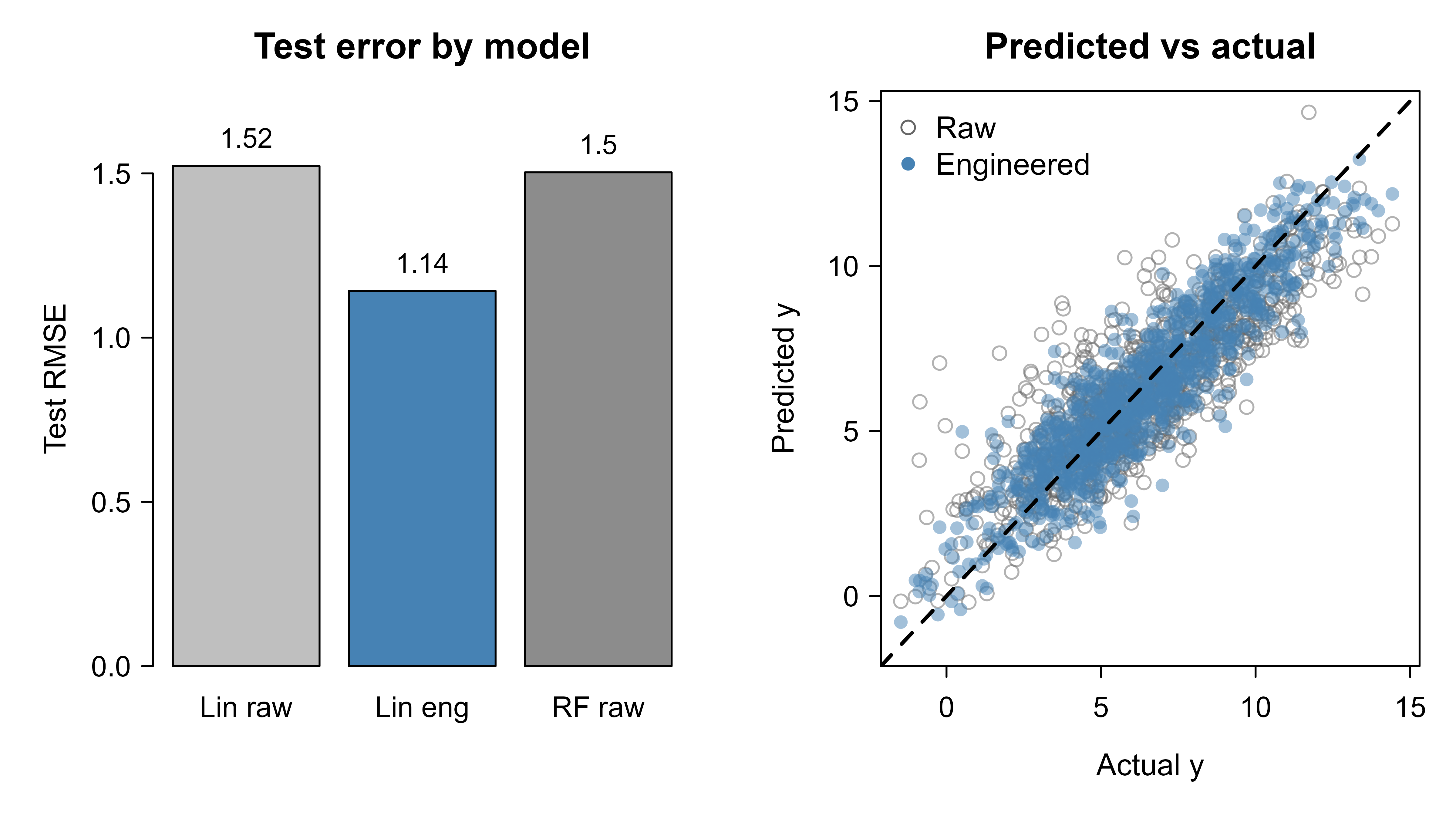
Table 83.1 collects the held-out root mean squared error for the three approaches. The engineered linear model improves substantially over the raw linear model and closes most or all of the gap to the random forest, despite being a simple, fully interpretable regression.
Show code
library(knitr)results<-data.frame( Model =c("Linear, raw features","Linear, engineered features","Random forest, raw features"), `Test RMSE` =round(c(rmse_base, rmse_eng, rmse_rf), 3), check.names =FALSE)kable(results, caption ="Held-out test RMSE for a linear model on raw features, the same linear model on engineered features, and a random forest reference. Lower is better.")
Table 83.1: Held-out test RMSE for a linear model on raw features, the same linear model on engineered features, and a random forest reference. Lower is better.
Model
Test RMSE
Linear, raw features
1.522
Linear, engineered features
1.142
Random forest, raw features
1.503
Figure 83.1 visualizes the same comparison two ways. The left panel shows the test RMSE as a bar for each model; the right panel plots predicted against actual outcomes for the raw and engineered linear models, where points hugging the diagonal indicate better predictions.
Show code
par(mfrow =c(1, 2), mar =c(4.2, 4.2, 2.5, 1))# Panel 1: RMSE bars.bp<-barplot(c(rmse_base, rmse_eng, rmse_rf), names.arg =c("Lin raw", "Lin eng", "RF raw"), ylab ="Test RMSE", main ="Test error by model", col =c("grey75", "steelblue", "grey55"), ylim =c(0, max(rmse_base, rmse_eng, rmse_rf)*1.15))text(bp, c(rmse_base, rmse_eng, rmse_rf), labels =round(c(rmse_base, rmse_eng, rmse_rf), 2), pos =3, cex =0.9)# Panel 2: predicted vs actual.lim<-range(c(test$y, pred_base, pred_eng))plot(test$y, pred_base, xlim =lim, ylim =lim, pch =1, col =adjustcolor("grey40", 0.5), xlab ="Actual y", ylab ="Predicted y", main ="Predicted vs actual")points(test$y, pred_eng, pch =16, col =adjustcolor("steelblue", 0.5))abline(0, 1, lty =2, lwd =2)legend("topleft", legend =c("Raw", "Engineered"), pch =c(1, 16), col =c("grey40", "steelblue"), bty ="n")
Figure 83.1: Left: held-out RMSE by model (shorter bars are better). Right: predicted versus actual for the raw linear model (open circles) and the engineered linear model (filled circles); the dashed line is perfect prediction. Engineered features pull the predictions toward the diagonal.
The lesson is not that linear models beat random forests, nor the reverse. It is that the representation handed to the model is doing real work. The engineered features encode the log scale, the interaction, the daily cycle, and the per-store effect that the raw columns hid, and a transparent linear model on those features competes with a black-box ensemble on the raw ones.
83.9 A note on doing this with recipes
The recipes package (part of tidymodels, see Chapter 90) lets you declare a feature pipeline once and have it refit correctly inside resampling, which removes most opportunities for leakage. The code below is illustrative; it expresses the same kinds of steps as the manual pipeline above. It is shown rather than run to keep this chapter’s executed output self-contained, but it is idiomatic and will run in a tidymodels session.
For shrunk target encoding inside cross-validation, vtreat::mkCrossFrameNExperiment (numeric outcome) and the embed package’s step_lencode_mixed provide out-of-fold encodings that avoid the leakage discussed above.
83.10 Practical guidance and pitfalls
A few habits separate feature engineering that helps from feature engineering that quietly hurts.
Learn every parameter on training data and freeze it. Scaling constants, imputation values, category levels, and target-encoding means are all parameters. Estimate them once on the training rows and apply the frozen values everywhere else.
Put the whole pipeline inside cross-validation. The performance number you trust is the one where feature steps were refit on each fold’s training portion. A pipeline that is leak-free on a single split can still leak if you re-estimate features on the full data before tuning.
Be deliberate about high cardinality. One-hot encoding a thousand-level variable creates a thousand columns and invites overfitting; target encoding collapses it to one but must be shrunk and computed out of fold. Pooling rare levels into an “other” bucket is a cheap, robust middle ground.
Prefer transforms that match the data’s shape. Log transforms for skewed positive variables, sine and cosine pairs for cyclical fields, and explicit interactions for known synergies usually beat throwing raw columns at a flexible model and hoping it finds the structure.
Keep missingness indicators. The fact that a value was missing is often predictive on its own, and an indicator column lets the model use it instead of trusting an imputed value as if observed.
Warning
Resist the temptation to engineer features by eyeballing the relationship between a candidate feature and the outcome on the full dataset. That inspection is itself a use of the outcome, and features chosen this way can look strong and generalize poorly. Choose feature ideas from domain knowledge and the training data, and let held-out data be the judge.
Note
More features are not always better. Each engineered column adds variance and a maintenance cost in production. After engineering, the predictor-reduction tools (Chapter 81) and regularization elsewhere in this book help prune the set back down to what earns its place.
83.11 Further reading
Kuhn, M. and Johnson, K. (2013). Applied Predictive Modeling. Springer. A thorough, practitioner-focused treatment of preprocessing, encoding, and resampling.
Kuhn, M. and Johnson, K. (2019). Feature Engineering and Selection: A Practical Approach for Predictive Models. CRC Press. The definitive book-length treatment, with extensive coverage of target encoding and leakage.
Micci-Barreca, D. (2001). “A preprocessing scheme for high-cardinality categorical attributes in classification and prediction problems.” ACM SIGKDD Explorations. The original target (impact) encoding paper.
Zheng, A. and Casari, A. (2018). Feature Engineering for Machine Learning. O’Reilly. A concise, example-driven tour of common transformations.
Kaufman, S., Rosset, S., and Perlich, C. (2012). “Leakage in data mining: Formulation, detection, and avoidance.” ACM Transactions on Knowledge Discovery from Data. A careful taxonomy of how leakage arises and how to prevent it.
Kuhn, M. and Wickham, H. (2020). Tidymodels and the recipes package documentation. The reference for declaring leak-safe preprocessing pipelines in R.
This is an empirical-Bayes style estimator: \(\lambda\) acts as a number of “pseudo-observations” pulling each level’s estimate toward the overall mean. Large \(n_\ell\) trusts the level’s own data; small \(n_\ell\) borrows strength from the global mean. Micci-Barreca (2001) introduced this encoding.↩︎
Source Code
# Feature Engineering {#sec-feature-engineering}```{r}#| include: falsesource("_common.R")```Most of this book is about models: how a spline bends, how a tree splits, how a network learns. Feature engineering is about the other half of the bargain, the part that decides what those models actually see. A model can only learn relationships that are expressible in the columns you hand it. If the signal lives in the interaction between two variables, in the hour of the day rather than the raw timestamp, or in a rare category that you have not encoded sensibly, then no amount of model tuning will recover it. Feature engineering is the work of shaping raw data into the representation that lets a model do its job.The payoff is large and often underappreciated. A practitioner who spends an afternoon constructing thoughtful features will frequently beat a practitioner who spends a week tuning hyperparameters on raw inputs. The features encode domain knowledge that the model cannot invent on its own, and they do so in a way that is cheap to compute and easy to inspect.::: {.callout-important title="Key idea"}A model learns a function of the features you give it, not of the data you wish you had given it. Feature engineering changes the input space so that the relationship you care about becomes easy for the model to express.:::This chapter walks through the core operations: scaling numeric variables, encoding categorical ones, building interactions, binning continuous predictors, extracting structure from dates and text, and handling missing values. Throughout, one theme recurs and deserves emphasis from the start: any transformation that uses the outcome, or that pools information across rows, must be learned on training data alone and then applied to validation data. Doing otherwise leaks information and inflates your performance estimates. We will build a small pipeline that does this correctly and show, with a before and after comparison, that good features improve a model on data where the truth is known.::: {.callout-note}The terms "feature" and "predictor" and "variable" are used interchangeably here. A feature is simply a column of the design matrix that the model consumes.:::## Notation and setupLet the training data consist of $n$ observations. For observation $i$ we write the outcome as $y_i$ and the raw inputs as a vector $\mathbf{x}_i$. A feature transformation is a function $\phi$ that maps raw inputs to a new feature vector $\mathbf{z}_i = \phi(\mathbf{x}_i)$. The model is then fit on the pairs $(\mathbf{z}_i, y_i)$ rather than on $(\mathbf{x}_i, y_i)$.The subtlety is that $\phi$ itself often has parameters estimated from data. A centering and scaling step needs a mean and a standard deviation; a target encoder needs category averages of $y$. We write these learned quantities as $\hat\theta$, estimated on the training set, so that the transformation is really $\phi(\cdot \,;\, \hat\theta)$. The cardinal rule is that $\hat\theta$ is estimated using training rows only, and the same fixed $\hat\theta$ is then used to transform validation and test rows.::: {.callout-warning}If $\hat\theta$ is estimated on the full dataset before splitting, information from the validation rows leaks into the features. This is the most common and most damaging feature-engineering mistake. We return to it in detail in the section on leakage.:::## Scaling numeric featuresMany learners are sensitive to the scale of their inputs. Distance-based methods such as $k$ nearest neighbors, kernel methods, and any penalized model such as ridge or lasso treat a variable measured in thousands very differently from one measured in fractions, purely because of the units. Standardization removes the units so that each feature contributes on comparable footing.The standard score, or $z$ score, of a feature centers it at zero and rescales it to unit variance:$$z_{ij} = \frac{x_{ij} - \hat\mu_j}{\hat\sigma_j},$$where $\hat\mu_j$ and $\hat\sigma_j$ are the mean and standard deviation of feature $j$ estimated on the training set. An alternative is min-max scaling, which maps each feature to the unit interval:$$\tilde{x}_{ij} = \frac{x_{ij} - \min_j}{\max_j - \min_j},$$with $\min_j$ and $\max_j$ again learned from training data. Standardization is the usual default because it is less sensitive to a single extreme value than min-max scaling, which is anchored to the most extreme observations.::: {.callout-tip title="Intuition"}Scaling does not change the information in a feature, only its units. It matters for models that compare features by magnitude (penalized regression, distance methods) and is irrelevant for models that are invariant to monotone rescaling of a single variable, such as decision trees.:::::: {.callout-tip title="When to use this"}Always scale for ridge, lasso, elastic net, support vector machines, $k$ nearest neighbors, principal components, and neural networks. You can usually skip it for tree-based models.:::For skewed positive variables, a log transform $x \mapsto \log(1 + x)$ often helps more than scaling, because it compresses a long right tail into a range where a linear model can use it. We apply exactly this idea in the demo.## Encoding categorical featuresA categorical variable takes one of a finite set of labels, and most models cannot consume labels directly. We need a numeric encoding. The two workhorses are one-hot encoding and target encoding, and they trade off in an instructive way.### One-hot encodingOne-hot encoding (also called dummy coding) replaces a categorical variable with $L$ levels by $L$ binary indicator columns, one per level, where the column for the observed level is one and the rest are zero. To avoid perfect collinearity in a model with an intercept, we drop one level and keep $L - 1$ columns:$$z_{i\ell} = \mathbb{1}\{\, x_i = \text{level } \ell \,\}, \qquad \ell = 1, \dots, L-1.$$One-hot encoding is faithful: it makes no assumption about an ordering or a relationship among levels, and the model is free to assign each level its own coefficient. Its weakness is dimensionality. A variable with thousands of levels (a zip code, a product id) produces thousands of sparse columns, which inflates the design matrix and can hurt models that struggle in high dimensions.::: {.callout-note}Always learn the set of levels on the training set. If a new level appears at prediction time, a fixed encoder must have a deliberate policy for it, such as mapping it to an "unseen" indicator or to all zeros. Silently failing on novel levels is a frequent production bug.:::### Target (impact) encodingTarget encoding replaces each level with a summary of the outcome for that level. For a numeric outcome and level $\ell$, the simplest version uses the within-level mean:$$\hat{m}_\ell = \frac{1}{n_\ell} \sum_{i : x_i = \ell} y_i,$$where $n_\ell$ is the number of training rows in level $\ell$. The categorical column is then replaced by the single numeric column $z_i = \hat m_{x_i}$. This collapses a high-cardinality variable into one informative feature.The danger is overfitting on rare levels: a level seen only once has a within-level mean equal to that single $y$, which is pure noise dressed up as signal. The remedy is shrinkage toward the global mean $\bar y$, weighting by how much data the level has:$$\hat{m}_\ell^{\text{shrunk}} = \frac{n_\ell \, \hat m_\ell + \lambda \, \bar y}{n_\ell + \lambda},$$where $\lambda \ge 0$ is a smoothing constant.^[This is an empirical-Bayes style estimator: $\lambda$ acts as a number of "pseudo-observations" pulling each level's estimate toward the overall mean. Large $n_\ell$ trusts the level's own data; small $n_\ell$ borrows strength from the global mean. Micci-Barreca (2001) introduced this encoding.] As $\lambda \to 0$ we recover the raw level mean; as $\lambda \to \infty$ every level collapses to $\bar y$.::: {.callout-warning}Target encoding uses the outcome, so it is the textbook source of leakage. The level means must be computed on training rows only, and ideally with out-of-fold estimation inside cross-validation, or the encoded feature will look far more predictive than it really is.:::## Interactions and binningTwo further operations expand what a model can express without changing the model itself.An interaction is a product of features, $z = x_j \, x_k$, that lets the effect of one variable depend on another. A linear model with only main effects is forced to assume that the slope on $x_j$ is the same at every value of $x_k$; adding the product term relaxes that. Tree ensembles discover interactions automatically through their splits, but linear and additive models need them supplied explicitly.Binning (discretization) replaces a continuous variable with the bin it falls into, turning it into a categorical feature. This lets a linear model fit a step function and so capture nonlinearity, and it can tame outliers by capping them into the end bins. The cost is a loss of resolution within each bin and a dependence on where the cut points fall.::: {.callout-tip title="Intuition"}Interactions and binning both add flexibility that the model could not otherwise represent. Interactions add it across variables; binning adds it within a variable. Splines (covered in the spline regression chapter, @sec-spline) are usually a smoother alternative to binning.:::## Date, time, and text featuresRaw timestamps and free text are rarely usable as is. A timestamp such as `2026-06-17 09:14:00` is a single large integer to a model, yet the useful signal is almost always in its parts: the hour of day, the day of week, whether it is a weekend, the month, the time since some reference event. Cyclical fields such as hour or month are often encoded with a sine and cosine pair so that hour 23 sits next to hour 0:$$z_{\sin} = \sin\!\left(\frac{2\pi h}{24}\right), \qquad z_{\cos} = \cos\!\left(\frac{2\pi h}{24}\right),$$for hour $h \in \{0, \dots, 23\}$. This pair places the 24 hours evenly on a circle, so the model sees that late night and early morning are close.Free text is commonly reduced to a bag of words: counts (or presence) of each token, optionally reweighted by inverse document frequency so that rare, discriminating words count more than ubiquitous ones. Modern alternatives replace counts with learned embeddings, covered in the embeddings and vector search chapter (@sec-embeddings-vector-search). The engineering principle is the same as for dates: explode the raw object into many simple, model-readable columns.## Handling missing valuesMissing entries must be resolved before most models will run. The two parts of a good strategy are imputation, filling in a value, and a missingness indicator, a binary flag recording that the value was originally absent.The simplest imputations replace a missing numeric value with the training mean or median, and a missing categorical value with the training mode or with an explicit "missing" level. More elaborate methods predict the missing entry from the other columns. Whatever the method, the imputation model is fit on training data and applied unchanged to validation data.Adding the indicator is valuable because the fact of missingness is itself often informative: an unfilled income field may correlate with the outcome regardless of what the true income was. Keeping the flag lets the model use that signal instead of pretending the imputed value was observed.::: {.callout-warning}Compute the imputation values (means, medians, modes) on the training set only. Imputing with the full-data mean before splitting leaks the validation rows into the training features, exactly the error the next section is about.:::## Leakage and cross-validationWe can now state the central discipline plainly. Several of the transformations above estimate parameters from data: scaling needs means and standard deviations, target encoding needs level means of the outcome, imputation needs column summaries. Every one of these $\hat\theta$ must be learned inside the training portion of each resampling split and then applied to the held-out portion. The held-out rows must never influence the transformation that is later applied to them.::: {.callout-important title="Key idea"}Treat the entire feature-engineering pipeline as part of the model. Whatever the model's fitting procedure is wrapped in cross-validation, the feature steps must be wrapped in the same loop, refit on each fold's training rows.:::The most insidious case is target encoding, because it touches the outcome directly. The clean solution is out-of-fold encoding: to encode a training row, use level means computed from the other folds, never from the row's own fold. The `recipes` and `vtreat` packages implement this. In the demo we keep the logic explicit and simple, computing the encoder on a training split and applying it to a disjoint test split, which is enough to expose the difference between honest and leaky feature engineering.::: {.callout-tip}A quick audit: list every pipeline step that computes a number from the data. For each, ask whether that number was computed using only training rows. If any step saw the validation or test rows, you have leakage.:::## Demonstration: a feature-engineering pipeline that helpsWe now build a small but complete example. The data are simulated so that we know the truth: the outcome depends on a log-scaled numeric variable, an interaction, a cyclical time field, and a high-cardinality categorical variable, with some values made missing. A linear model fit on the raw columns cannot express these relationships well. The same linear model fit on engineered features should do much better, and a flexible model (random forest) gives us a reference point.We hold out a test set once, learn every transformation parameter on the training set only, and apply the frozen transformation to the test set. This mirrors the leakage discipline above.```{r feature-engineering-simulate}set.seed(2026)n <-4000# High-cardinality categorical: 50 "stores", each with its own latent effect.n_levels <-50store_effect <-rnorm(n_levels, mean =0, sd =1.5)store <-sample(seq_len(n_levels), size = n, replace =TRUE)# Skewed positive numeric: spend, used on the log scale by the truth.spend <-rexp(n, rate =1/50)# Cyclical time field: hour of day, with a smooth daily rhythm.hour <-sample(0:23, size = n, replace =TRUE)daily <-sin(2* pi * hour /24)# A second numeric predictor that interacts with log spend.promo <-rbinom(n, size =1, prob =0.4)# True signal (regression). Note: log(spend), an interaction, the cycle,# and the per-store effect all matter; raw columns hide most of this.lin <-2.0+0.9*log1p(spend) +0.8* promo *log1p(spend) +1.2* daily + store_effect[store]y <- lin +rnorm(n, sd =1.0)dat <-data.frame(y = y,spend = spend,hour = hour,promo =factor(promo),store =factor(store))# Inject missingness into spend (about 10%), missing completely at random.miss_idx <-sample(seq_len(n), size =round(0.10* n))dat$spend[miss_idx] <-NAstr(dat)```We split once into training and test sets. Every transformation parameter below is learned from `train` only.```{r feature-engineering-split}set.seed(7)test_id <-sample(seq_len(nrow(dat)), size =round(0.25*nrow(dat)))train <- dat[-test_id, ]test <- dat[test_id, ]c(train_rows =nrow(train), test_rows =nrow(test))```### The baseline: raw featuresThe naive model uses the columns as they arrive. Missing `spend` values are dropped by `lm`, the high-cardinality `store` factor becomes many dummy columns, and no interaction or cyclical encoding is supplied. We impute the missing `spend` with the training mean only (so the baseline is not crippled by dropped rows) and otherwise feed raw columns.```{r feature-engineering-baseline}# Training-set mean for imputation (learned on train only).spend_mean <-mean(train$spend, na.rm =TRUE)impute_spend <-function(df) { s <- df$spend s[is.na(s)] <- spend_mean s}train_base <-data.frame(y = train$y,spend =impute_spend(train),hour = train$hour,promo = train$promo,store = train$store)test_base <-data.frame(y = test$y,spend =impute_spend(test),hour = test$hour,promo = test$promo,store = test$store)fit_base <-lm(y ~ spend + hour + promo + store, data = train_base)rmse <-function(actual, pred) sqrt(mean((actual - pred)^2))pred_base <-predict(fit_base, newdata = test_base)rmse_base <-rmse(test_base$y, pred_base)rmse_base```### The engineered pipelineNow we build features that match the structure of the problem, learning every parameter on `train`. The steps are: median imputation of `spend` plus a missingness flag; a log transform of `spend`; standardization of the log-spend; a promo by log-spend interaction; sine and cosine of `hour`; and shrunk target encoding of `store`. We write the encoder as a function so the exact same learned values apply to the test set.```{r feature-engineering-pipeline}# --- Parameters learned on the training set only ---# 1. Imputation value for spend (median is robust to the long right tail).spend_median <-median(train$spend, na.rm =TRUE)# 2. Standardization parameters for log-spend, computed AFTER imputation# on the training set.train_logspend_raw <-log1p(ifelse(is.na(train$spend), spend_median, train$spend))ls_mean <-mean(train_logspend_raw)ls_sd <-sd(train_logspend_raw)# 3. Shrunk target encoding for store (out-of-sample safe: train means only).global_mean <-mean(train$y)lambda <-20# smoothing strengthagg <-aggregate(y ~ store, data = train, FUN =function(v) c(m =mean(v), n =length(v)))store_stats <-data.frame(store = agg$store,m = agg$y[, "m"],n = agg$y[, "n"])store_stats$encoded <-with( store_stats, (n * m + lambda * global_mean) / (n + lambda))store_map <-setNames(store_stats$encoded, as.character(store_stats$store))# --- The transformation function: applies frozen parameters to any data frame ---engineer <-function(df) { spend_missing <-as.integer(is.na(df$spend)) spend_imp <-ifelse(is.na(df$spend), spend_median, df$spend) log_spend <-log1p(spend_imp) log_spend_z <- (log_spend - ls_mean) / ls_sd# Target encoding: unseen levels fall back to the global mean. enc <- store_map[as.character(df$store)] enc[is.na(enc)] <- global_meandata.frame(y = df$y,log_spend_z = log_spend_z,spend_missing = spend_missing,promo =as.integer(as.character(df$promo)),promo_x_logspend =as.integer(as.character(df$promo)) * log_spend_z,hour_sin =sin(2* pi * df$hour /24),hour_cos =cos(2* pi * df$hour /24),store_enc =as.numeric(enc) )}train_eng <-engineer(train)test_eng <-engineer(test)fit_eng <-lm(y ~ ., data = train_eng)pred_eng <-predict(fit_eng, newdata = test_eng)rmse_eng <-rmse(test_eng$y, pred_eng)rmse_eng```### A flexible-model referenceA random forest on the raw columns gives a sense of how much signal a strong learner can extract without hand-built features. It handles the interaction and the categorical natively, though it still benefits from the missingness being resolved.```{r feature-engineering-rf}library(randomForest)set.seed(11)# Random forests need complete cases; reuse the simple training-mean imputation.train_rf <- train_basetest_rf <- test_basefit_rf <-randomForest(y ~ spend + hour + promo + store,data = train_rf, ntree =300)pred_rf <-predict(fit_rf, newdata = test_rf)rmse_rf <-rmse(test_rf$y, pred_rf)rmse_rf```### Results@tbl-feature-engineering-results collects the held-out root mean squared error for the three approaches. The engineered linear model improves substantially over the raw linear model and closes most or all of the gap to the random forest, despite being a simple, fully interpretable regression.```{r tbl-feature-engineering-results}library(knitr)results <-data.frame(Model =c("Linear, raw features","Linear, engineered features","Random forest, raw features" ),`Test RMSE`=round(c(rmse_base, rmse_eng, rmse_rf), 3),check.names =FALSE)kable( results,caption ="Held-out test RMSE for a linear model on raw features, the same linear model on engineered features, and a random forest reference. Lower is better.")```@fig-feature-engineering-compare visualizes the same comparison two ways. The left panel shows the test RMSE as a bar for each model; the right panel plots predicted against actual outcomes for the raw and engineered linear models, where points hugging the diagonal indicate better predictions.```{r fig-feature-engineering-compare, fig.width=8, fig.height=4.5, fig.cap="Left: held-out RMSE by model (shorter bars are better). Right: predicted versus actual for the raw linear model (open circles) and the engineered linear model (filled circles); the dashed line is perfect prediction. Engineered features pull the predictions toward the diagonal."}par(mfrow =c(1, 2), mar =c(4.2, 4.2, 2.5, 1))# Panel 1: RMSE bars.bp <-barplot(c(rmse_base, rmse_eng, rmse_rf),names.arg =c("Lin raw", "Lin eng", "RF raw"),ylab ="Test RMSE",main ="Test error by model",col =c("grey75", "steelblue", "grey55"),ylim =c(0, max(rmse_base, rmse_eng, rmse_rf) *1.15))text(bp, c(rmse_base, rmse_eng, rmse_rf),labels =round(c(rmse_base, rmse_eng, rmse_rf), 2),pos =3, cex =0.9)# Panel 2: predicted vs actual.lim <-range(c(test$y, pred_base, pred_eng))plot(test$y, pred_base,xlim = lim, ylim = lim,pch =1, col =adjustcolor("grey40", 0.5),xlab ="Actual y", ylab ="Predicted y",main ="Predicted vs actual")points(test$y, pred_eng, pch =16, col =adjustcolor("steelblue", 0.5))abline(0, 1, lty =2, lwd =2)legend("topleft",legend =c("Raw", "Engineered"),pch =c(1, 16), col =c("grey40", "steelblue"), bty ="n")```The lesson is not that linear models beat random forests, nor the reverse. It is that the representation handed to the model is doing real work. The engineered features encode the log scale, the interaction, the daily cycle, and the per-store effect that the raw columns hid, and a transparent linear model on those features competes with a black-box ensemble on the raw ones.## A note on doing this with `recipes`The `recipes` package (part of `tidymodels`, see @sec-tidymodels-framework) lets you declare a feature pipeline once and have it refit correctly inside resampling, which removes most opportunities for leakage. The code below is illustrative; it expresses the same kinds of steps as the manual pipeline above. It is shown rather than run to keep this chapter's executed output self-contained, but it is idiomatic and will run in a `tidymodels` session.```{r feature-engineering-recipe, eval=FALSE}library(recipes)library(rsample)rec <-recipe(y ~ spend + hour + promo + store, data = train) |>step_impute_median(spend) |>step_indicate_na(spend) |># missingness flagstep_log(spend, offset =1) |># log1p transformstep_normalize(spend) |># center and scalestep_mutate(hour_sin =sin(2* pi * hour /24)) |>step_mutate(hour_cos =cos(2* pi * hour /24)) |>step_rm(hour) |>step_interact(terms =~ spend:promo) |>step_dummy(promo) |>step_other(store, threshold =0.01) |># pool rare storesstep_dummy(store)# Prep on TRAIN only, then bake TRAIN and TEST with the frozen estimates.prepped <-prep(rec, training = train)train_baked <-bake(prepped, new_data =NULL)test_baked <-bake(prepped, new_data = test)```For shrunk target encoding inside cross-validation, `vtreat::mkCrossFrameNExperiment` (numeric outcome) and the `embed` package's `step_lencode_mixed` provide out-of-fold encodings that avoid the leakage discussed above.## Practical guidance and pitfallsA few habits separate feature engineering that helps from feature engineering that quietly hurts.Learn every parameter on training data and freeze it. Scaling constants, imputation values, category levels, and target-encoding means are all parameters. Estimate them once on the training rows and apply the frozen values everywhere else.Put the whole pipeline inside cross-validation. The performance number you trust is the one where feature steps were refit on each fold's training portion. A pipeline that is leak-free on a single split can still leak if you re-estimate features on the full data before tuning.Be deliberate about high cardinality. One-hot encoding a thousand-level variable creates a thousand columns and invites overfitting; target encoding collapses it to one but must be shrunk and computed out of fold. Pooling rare levels into an "other" bucket is a cheap, robust middle ground.Prefer transforms that match the data's shape. Log transforms for skewed positive variables, sine and cosine pairs for cyclical fields, and explicit interactions for known synergies usually beat throwing raw columns at a flexible model and hoping it finds the structure.Keep missingness indicators. The fact that a value was missing is often predictive on its own, and an indicator column lets the model use it instead of trusting an imputed value as if observed.::: {.callout-warning}Resist the temptation to engineer features by eyeballing the relationship between a candidate feature and the outcome on the full dataset. That inspection is itself a use of the outcome, and features chosen this way can look strong and generalize poorly. Choose feature ideas from domain knowledge and the training data, and let held-out data be the judge.:::::: {.callout-note}More features are not always better. Each engineered column adds variance and a maintenance cost in production. After engineering, the predictor-reduction tools (@sec-predictor-reduction) and regularization elsewhere in this book help prune the set back down to what earns its place.:::## Further reading- Kuhn, M. and Johnson, K. (2013). *Applied Predictive Modeling*. Springer. A thorough, practitioner-focused treatment of preprocessing, encoding, and resampling.- Kuhn, M. and Johnson, K. (2019). *Feature Engineering and Selection: A Practical Approach for Predictive Models*. CRC Press. The definitive book-length treatment, with extensive coverage of target encoding and leakage.- Micci-Barreca, D. (2001). "A preprocessing scheme for high-cardinality categorical attributes in classification and prediction problems." *ACM SIGKDD Explorations*. The original target (impact) encoding paper.- Zheng, A. and Casari, A. (2018). *Feature Engineering for Machine Learning*. O'Reilly. A concise, example-driven tour of common transformations.- Kaufman, S., Rosset, S., and Perlich, C. (2012). "Leakage in data mining: Formulation, detection, and avoidance." *ACM Transactions on Knowledge Discovery from Data*. A careful taxonomy of how leakage arises and how to prevent it.- Kuhn, M. and Wickham, H. (2020). *Tidymodels* and the `recipes` package documentation. The reference for declaring leak-safe preprocessing pipelines in R.