A model in production is only as good as the features it receives at the moment it has to predict. Most of the work in an applied ML system is not the model: it is computing, storing, and serving features reliably, and doing so the same way during training as during serving. A feature store is the piece of infrastructure that addresses this. It is a system for defining features once, computing them once, and reusing them across many models and across both training and serving, while guaranteeing two properties that are easy to violate by hand: that the features used to train a model match the features served at prediction time, and that the feature values used for a training label were knowable at the time the label was generated.
This chapter explains the offline/online pattern that feature stores implement, the two correctness problems they solve (training-serving skew and point-in-time correctness), and the operations they support (registration, materialization, reuse). Production feature stores (Feast, Tecton, Databricks Feature Store, Vertex AI Feature Store) are external systems, so chunks that reference them are marked eval=FALSE and written so a reader can run them in a configured environment. To teach the core ideas with code that runs, the chapter builds a small feature-store abstraction in base R and data.table: you register feature functions, materialize a feature table, and perform a point-in-time join that avoids label leakage.
Intuition
Think of a feature store as a shared kitchen for an ML team. Instead of every cook (model) buying and chopping the same vegetables (features) in their own way, the ingredients are prepared once, to one recipe, and handed to everyone. The two guarantees the store enforces are that the dish tastes the same whether you order it now or had it last month (no training-serving skew), and that no recipe secretly uses an ingredient that had not yet arrived in the pantry (no leakage).
By the end of the chapter you should be able to state the two correctness problems precisely, explain why the offline and online stores hold the same features in different shapes, and read (and modify) a working as-of join that produces a leakage-free training table.
119.1 Where this fits in a modern ML/AI workflow
Consider the lifecycle of a single prediction problem, say predicting whether a customer will churn. Raw events arrive continuously: logins, purchases, support tickets. A model does not consume raw events; it consumes features such as “number of logins in the last 7 days” or “days since last purchase.” Those features have to be computed from the raw events, a process treated in depth in the feature engineering chapter (Chapter 83). The trouble is that they are computed in (at least) two very different places.
During training, you compute features in batch over historical data, typically in a data warehouse or a data.table/Spark job (see the Spark and sparklyr chapter, Chapter 96), for millions of rows at once.
During serving, you compute the same features for one customer at a time, on demand, with a latency budget of milliseconds, often from a different code path and a different data store.
When the same feature is implemented twice, by two people, in two languages, against two storage systems, the two implementations drift. The model was trained on one definition and is served another. This is training-serving skew,1 and it is one of the most common and most damaging failure modes in deployed ML. A feature store removes the duplication: a feature is defined once, and the same definition feeds both the offline (training) and online (serving) paths.
Warning
Skew rarely announces itself. The model keeps returning predictions, the service keeps responding, and only the quality quietly erodes. Because nothing crashes, skew can persist for months before anyone connects falling business metrics to a feature whose serving-time definition drifted from its training-time twin.
A second problem is subtler. To train a supervised model you assemble rows of the form (features, label). The label is observed at some time \(t\). The features must reflect only information available strictly before \(t\). If any feature accidentally includes data from on or after \(t\), the model learns from the future, scores beautifully in offline evaluation, and fails in production. This is label leakage,2 and the discipline that prevents it is point-in-time correctness: every feature value joined to a label must be the value that was current as of the label’s timestamp. Doing this join by hand is error prone; a feature store builds it into the materialization step.
Key idea
Training-serving skew is about computing a feature the same way in two places. Point-in-time correctness is about computing it as of the right moment in time. The first keeps offline and online agreeing; the second keeps the past from peeking at the future. A feature store exists to enforce both automatically rather than leaving them to careful but fallible hand-coding.
So the feature store sits between raw data and the model, on both the training and serving paths, as the single source of truth for feature values:
raw events --> feature definitions --> offline store (history) --> training data
                                   \--> online store (latest)   --> serving
This pattern matters for data scientists (consistent, reusable features across projects), data engineers (one materialization pipeline rather than many ad hoc ones), and ML/AI engineers (a contract that keeps training and serving aligned).
119.2 The two correctness problems, stated precisely
Let raw observations be timestamped events. Write a feature as a function of an entity and a timestamp. Let \(e\) index an entity (a customer, a device, a stock ticker) and let \(t\) be a timestamp. A feature is a function
where \(f(e, t)\) uses only events for entity \(e\) with event time strictly less than \(t\). The strict inequality is the whole point: at decision time \(t\) you do not yet know events that occur at \(t\) or later.
Note
Writing a feature as a function of an entity and a timestamp is the move that makes correctness checkable. A feature is not just “the customer’s login count”; it is “the customer’s login count as known at time \(t\).” Once the timestamp is an explicit argument, the rule “use only events with time \(< t\)” is something you can read off the code and test, rather than a convention you hope everyone followed.
119.2.1 Training-serving skew
Let \(f^{\text{off}}\) be the offline (batch) implementation of a feature and \(f^{\text{on}}\) the online (serving) implementation. Skew is any systematic difference
that is nonzero for reasons other than legitimately newer data. Sources include different code, different rounding or null handling, different time-zone conventions, and different window boundaries (inclusive versus exclusive). The model was fit on the distribution of \(f^{\text{off}}\), so any nonzero \(\Delta\) at serving time shifts the input distribution and degrades predictions, often silently. A feature store drives \(\Delta \to 0\) by construction: there is one function, materialized to the offline store for training and to the online store for serving.
119.2.2 Point-in-time correctness
Suppose a label \(y_i\) for entity \(e_i\) is observed at time \(t_i\). We want the feature vector that was current “as of” \(t_i\). For a feature with values recorded at event times \(s_1 < s_2 < \cdots\), the point-in-time value is
\[
f(e_i, t_i) = \text{value recorded at } \max\{\, s_k : s_k < t_i \,\},
\]
that is, the most recent value strictly before the label time. The join that assembles a training table out of a label table and one or more feature tables, taking for each label the latest feature row before the label time, is an as-of join (also called a backward or rolling join). A naive equi-join on the entity alone, ignoring time, would attach the latest known feature value, which may post-date the label and leak the future. The as-of join is the operational form of point-in-time correctness.
Intuition
Picture each entity’s feature history as a row of stepping stones laid out along a time axis, one stone per recorded value. The label sits at its own point on that axis. The as-of join walks backward from the label and steps onto the nearest stone behind it. A plain join, by contrast, always jumps to the last stone in the row, even if that stone lies ahead of the label, which is exactly how the future leaks in.
Define leakage for a single feature as using \(f(e_i, t_i')\) for some \(t_i' \ge t_i\). The damage is that the offline estimate of generalization error is optimistically biased: if \(\hat{R}_{\text{leak}}\) is the risk estimated with leaked features and \(R\) is the true deployed risk, then typically \(\hat{R}_{\text{leak}} \ll R\), and the gap is not detectable from the offline split alone, because the split shares the leak.
119.3 Offline store and online store
A feature store keeps two copies of the same features because training and serving ask very different questions of the data. Training asks one enormous historical question all at once; serving asks tiny current questions one at a time. The two stores are tuned for those two shapes of demand.
The offline store holds the full history of feature values, keyed by entity and event time. It is optimized for large scans: “give me, for these ten million (entity, label-time) pairs, the point-in-time feature values.” It backs training and batch scoring. In practice it is a columnar warehouse or a set of partitioned files.
The online store holds only the latest value of each feature per entity, keyed by entity. It is optimized for low-latency key lookups: “give me the current feature vector for entity 12345” in a few milliseconds. It backs real-time serving. In practice it is a key-value store.
Materialization is the process that runs the feature definitions over raw data and writes the results: the full timeline to the offline store, and the latest snapshot per entity to the online store. Because both are written from the same definitions, the online value an entity is served equals the offline value that would be recorded for that entity at the same time, which is exactly the no-skew property.
Key idea
The online store is not a separately written system; it is a projection of the offline store down to “latest row per entity.” That single fact is what guarantees no skew. If the online values came from a different code path, all bets would be off. Keep this in mind when you read the runnable code later: we build online_store by literally taking the last row per customer from offline_store.
Table 119.1 contrasts the two stores along the dimensions that drive their different designs.
Table 119.1: Offline and online stores hold the same feature definitions but are tuned for different shapes of demand: large historical scans for training versus single-key lookups for serving.
Aspect
Offline store
Online store
Contents
full history of feature values
latest value per entity
Key
(entity, event time)
entity
Access pattern
large batch scans, as-of joins
single-key lookups
Latency target
seconds to minutes (throughput)
milliseconds (per request)
Backs
training, batch scoring
real-time serving
Typical storage
columnar warehouse, partitioned files
key-value store
Freshness
as of last batch materialization
as of last streaming/batch update
The feature definition is shared across both columns; only the storage and access pattern differ. That sharing is what a feature store buys you.
119.4 Feature reuse
Correctness is the headline benefit, but reuse is the one that pays the operational bills. A feature such as “7-day login count” is useful for churn prediction, for fraud scoring, and for a recommendation model. Without a feature store, each team recomputes it, with the attendant risk of subtle differences and duplicated compute. With a feature store, the feature is registered once under a name, materialized once, and referenced by name from every model. The unit of reuse is the named feature (or a named group of features sharing an entity and update cadence, often called a feature view or feature group). Reuse reduces compute, reduces skew across models, and makes lineage auditable: you can ask which models depend on a feature before you change it.
Tip
Treat a feature definition like a published API. Once several models reference logins_7d by name, changing what that name computes silently breaks all of them. The lineage a feature store records (“which models read this feature?”) is exactly what lets you change a definition deliberately instead of by accident.
119.5 A production feature store: Feast (eval=FALSE)
Before building our own, it helps to see what the real thing looks like, so the vocabulary (entity, source, feature view, materialization) lands on something concrete. The following sketch uses Feast, an open-source feature store, to show the shape of a real definition. It will not run here because feast (a Python package, driven from R via reticulate) and a configured store are not part of this environment. The code is idiomatic and current so it can be adapted in a configured project.
When to use this
Reach for a managed store like Feast when you actually have a low-latency online serving path, several models or teams sharing features, or event-timestamped data where point-in-time joins are easy to botch. For a single batch-scored model trained and served from the same warehouse, the lighter data.table approach later in this chapter is usually enough.
Show code
# Driven from R through reticulate; requires a configured Feast repo.library(reticulate)feast<-import("feast")# An entity is the join key for a group of features.customer<-feast$Entity(name ="customer_id", join_keys =list("customer_id"))# A data source points at the offline store (here, parquet files with# an event timestamp column used for point-in-time joins).source<-feast$infra$offline_stores$file_source$FileSource( path ="data/customer_features.parquet", timestamp_field ="event_timestamp")# A FeatureView is a named, reusable group of features for one entity.Field<-feast$FieldFloat32<-feast$types$Float32Int64<-feast$types$Int64customer_features<-feast$FeatureView( name ="customer_activity", entities =list(customer), ttl =reticulate::import("datetime")$timedelta(days =7L), schema =list(Field(name ="logins_7d", dtype =Int64),Field(name ="days_since_buy", dtype =Float32)), online =TRUE, source =source)
Training data is then assembled with a point-in-time join driven by an “entity dataframe” of (entity, label-timestamp) rows, and serving reads the latest values per entity from the online store.
Show code
store<-feast$FeatureStore(repo_path =".")# Offline: point-in-time-correct training data. Feast joins each label# row to the latest feature values strictly before its event_timestamp.entity_df<-data.frame( customer_id =c(1L, 2L, 3L), event_timestamp =as.POSIXct(c("2026-01-10", "2026-01-12", "2026-01-15"), tz ="UTC"))training<-store$get_historical_features( entity_df =entity_df, features =list("customer_activity:logins_7d","customer_activity:days_since_buy"))$to_df()# Push the latest values to the online store, then serve with low latency.store$materialize_incremental(end_date =reticulate::import("datetime")$datetime$now())online<-store$get_online_features( features =list("customer_activity:logins_7d"), entity_rows =list(list(customer_id =1L)))$to_dict()
The two reads, get_historical_features (offline, point-in-time) and get_online_features (online, latest), use the same customer_activity definition, which is how Feast prevents skew. The rest of the chapter implements this same contract in base R so you can see exactly what the as-of join does.
119.6 A runnable feature-store abstraction in base R and data.table
The next chunks run. They build a minimal feature store: a registry of feature functions, a materializer that computes the offline history and the online latest snapshot, and a point-in-time join that assembles training data without leakage. The implementation is small enough to read in full, and it exercises the same operations a production store exposes.
The plan mirrors the three operations a production store exposes: register feature definitions, materialize them into offline and online stores, and join them to labels point-in-time. We build each piece in turn and watch the output, so by the end the abstract contract from the first half of the chapter has a concrete counterpart you can run.
We start with raw events for a few customers and a registry that maps feature names to functions of an entity’s event history and a timestamp t. Each feature function uses only events strictly before t, which enforces \(f(e, t)\) depending on the past only.
The registry is just a named list of functions. Registering a feature stores its definition once; every downstream use refers to it by name, which is the reuse property. Each function receives ev, the events for one entity, and t, the as-of timestamp, and returns a scalar computed only from events before t.
Show code
feature_registry<-new.env()register_feature<-function(name, fun){stopifnot(is.function(fun))assign(name, fun, envir =feature_registry)invisible(name)}list_features<-function()ls(feature_registry)# Each feature uses ONLY events with event_time < t (strictly before).register_feature("logins_7d", function(ev, t){win<-ev[event_time<t&event_time>=t-7*86400&kind=="login"]nrow(win)})register_feature("total_spend", function(ev, t){past<-ev[event_time<t&kind=="purchase"]if(nrow(past)==0)0elsesum(past$amount)})register_feature("days_since_event", function(ev, t){past<-ev[event_time<t]if(nrow(past)==0)NA_real_elseas.numeric(difftime(t, max(past$event_time), units ="days"))})list_features()#> [1] "days_since_event" "logins_7d" "total_spend"
Materialization runs every registered feature for a set of (entity, timestamp) pairs. The offline store is the full history: we evaluate features on a grid of timestamps per entity, producing a timeline. The online store keeps only the latest row per entity, which is what serving would read.
Now the point-in-time join, the heart of the whole exercise. We have a label table with one (customer, label-time, label) row each. For each label we want the offline feature row with the largest event_timestamp strictly less than the label time. data.table’s rolling join does exactly this when we roll the feature times backward onto the label times.3 The guard for strict inequality matters: a feature row stamped exactly at the label time would represent information not yet available, so we exclude equality.
Show code
# Labels observed at specific times (the prediction targets).labels<-data.table( customer_id =c(1L, 2L, 3L, 4L, 5L), label_time =as.POSIXct(c("2026-01-18", "2026-01-09", "2026-01-27","2026-01-14", "2026-01-22"), tz ="UTC"), churned =c(1L, 0L, 1L, 0L, 1L))point_in_time_join<-function(labels, offline_store){L<-copy(labels); L[, join_time:=label_time]F<-copy(offline_store); F[, join_time:=event_timestamp]setkey(L, customer_id, join_time)setkey(F, customer_id, join_time)# Roll feature rows backward onto each label time: take the latest# feature row with join_time <= label_time, per customer.joined<-F[L, roll =TRUE]# Enforce STRICT inequality (no feature stamped exactly at label_time).joined[event_timestamp==label_time,c("logins_7d", "total_spend", "days_since_event"):=NA]joined[, .(customer_id, label_time, churned,logins_7d, total_spend, days_since_event)]}training<-point_in_time_join(labels, offline_store)training#> Key: <customer_id>#> customer_id label_time churned logins_7d total_spend days_since_event#> <int> <POSc> <int> <int> <num> <num>#> 1: 1 2026-01-18 1 2 0.00 2#> 2: 2 2026-01-09 0 0 41.68 2#> 3: 3 2026-01-27 1 1 159.13 5#> 4: 4 2026-01-14 0 1 72.69 3#> 5: 5 2026-01-22 1 1 174.24 3
Each training row now carries the feature values that were current strictly before its label time, which is the point-in-time-correct training table a model would be fit on.
To show why this matters, we contrast it with the leaky join: a plain merge that takes each customer’s latest known feature row regardless of the label time. For customers whose label time is early, the latest features post-date the label and leak the future.
Show code
# Leaky alternative: attach the LATEST feature row per customer,# ignoring the label time. This uses information from after label_time.leaky_join<-function(labels, online_store){merge(labels, online_store[, .(customer_id, logins_7d,total_spend, days_since_event)], by ="customer_id", all.x =TRUE)}leaky<-leaky_join(labels, online_store)# Compare total_spend under the two joins. Leakage shows up as a# feature value that could not have been known at label_time.cmp<-merge(training[, .(customer_id, label_time, pit_spend =total_spend)],leaky[, .(customer_id, leak_spend =total_spend)], by ="customer_id")cmp[, leaked:=leak_spend>pit_spend|is.na(pit_spend)]cmp#> Key: <customer_id>#> customer_id label_time pit_spend leak_spend leaked#> <int> <POSc> <num> <num> <lgcl>#> 1: 1 2026-01-18 0.00 0.00 FALSE#> 2: 2 2026-01-09 41.68 293.95 TRUE#> 3: 3 2026-01-27 159.13 283.74 TRUE#> 4: 4 2026-01-14 72.69 108.60 TRUE#> 5: 5 2026-01-22 174.24 174.24 FALSE
The leaked column flags the rows where the leaky join attached a larger (later) spend than was knowable at the label time. A model trained on leak_spend would appear to predict churn well offline and then underperform in production, because at serving time only the point-in-time value is available.
Warning
The most dangerous part of leakage is that the leaky training table contains no obvious tell. The numbers are valid spends for real customers; they are simply spends from the wrong side of the label time. You cannot catch this by inspecting the table for impossible values. You catch it by enforcing the as-of rule in the join, which is exactly why pushing that rule into shared infrastructure beats trusting each analyst to remember it.
119.6.1 A figure: leakage inflates apparent accuracy
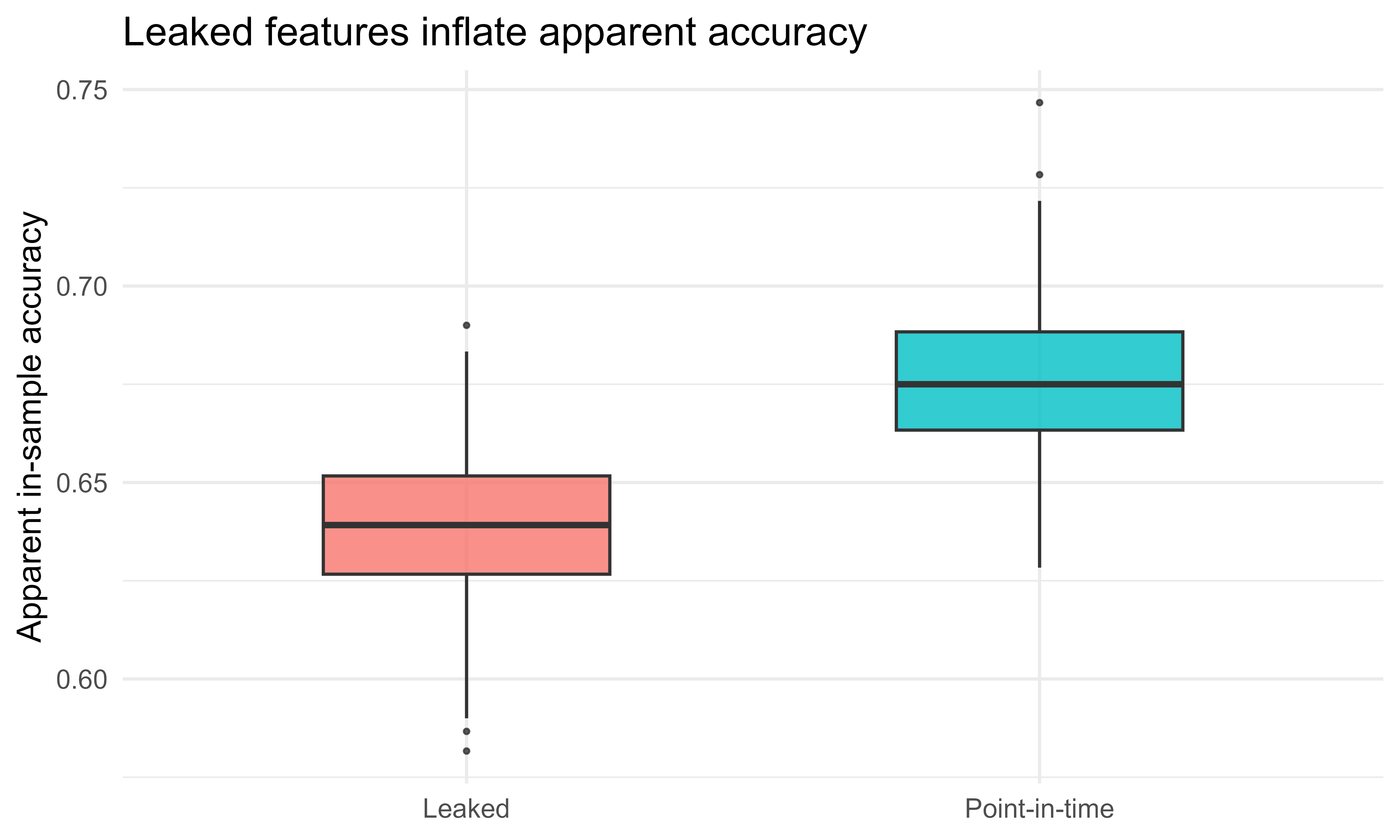
To make the cost of leakage concrete, we simulate a labeled dataset where the true signal is a point-in-time feature, then fit a simple logistic model twice: once on point-in-time features and once on leaked (future-peeking) features. We compare the apparent training accuracy. Leakage inflates it, which is precisely the optimistic bias \(\hat{R}_{\text{leak}} \ll R\) described earlier. Figure 119.1 shows the result.
Show code
suppressPackageStartupMessages(library(ggplot2))set.seed(7)simulate_once<-function(n=600){# Each unit has a label time and an underlying activity rate.rate<-runif(n, 0.2, 2)# Point-in-time feature: activity observed strictly before label time.x_pit<-rpois(n, lambda =rate)# Future increment that occurs AT/AFTER the label time (leakage if used).x_future<-rpois(n, lambda =rate)x_leak<-x_pit+x_future# Label depends only on the true (point-in-time) signal.p<-plogis(-1+0.9*x_pit)y<-rbinom(n, 1, p)acc<-function(x){fit<-glm(y~x, family =binomial)pred<-as.integer(predict(fit, type ="response")>0.5)mean(pred==y)}c(point_in_time =acc(x_pit), leaked =acc(x_leak))}res<-replicate(200, simulate_once())df<-data.frame( features =rep(c("Point-in-time", "Leaked"), each =ncol(res)), accuracy =c(res["point_in_time", ], res["leaked", ]))ggplot(df, aes(x =features, y =accuracy, fill =features))+geom_boxplot(width =0.5, alpha =0.8, outlier.size =0.6)+labs(x =NULL, y ="Apparent in-sample accuracy", title ="Leaked features inflate apparent accuracy")+theme_minimal(base_size =12)+theme(legend.position ="none")
Figure 119.1: Apparent in-sample accuracy under point-in-time-correct features versus leaked features that peek at post-label data. Leakage inflates the apparent accuracy; the gap is invisible from the offline split alone, which is why it is dangerous.
The leaked features score higher in-sample because they encode part of the future the label was drawn from. In deployment only the point-in-time features exist, so the leaked model’s real accuracy collapses toward the point-in-time model’s, and the offline evaluation gave no warning. The feature store’s as-of join is what keeps the training table on the honest (left) side of this picture.
119.7 Practical guidance, pitfalls, and when to use it
A feature store is worth its operational weight when you have real-time or low-latency serving (so an online path exists and can diverge from the offline path), when several models or teams share features (so reuse and a single definition pay off), or when point-in-time correctness is easy to get wrong (event-timestamped data, slowly changing entities, windowed aggregates). If you only ever score in batch from the same warehouse you train on, with one model and one team, a disciplined feature pipeline in data.table or dbplyr may be enough, and a full feature store can be over-engineering.
Pitfalls to watch for.
Equality at the boundary. The as-of join must use strict inequality (feature time \(<\) label time). Allowing equality lets a feature stamped exactly at the label time leak. Decide window boundaries (inclusive or exclusive) once and apply them identically offline and online.
Timestamp semantics. Event time (when the thing happened) is not ingestion time (when you recorded it). Point-in-time correctness needs the time the information became available to the system, which for late-arriving data is the ingestion time, not the event time. Mixing the two reintroduces leakage.
Time zones and clock skew. A feature defined with a local-time daily window and served with a UTC window will skew silently. Store and compute in one zone (UTC is the safe default) everywhere.
Online/offline drift in materialization cadence. The online store is only as fresh as the last materialization. If serving expects a 7-day window updated hourly but materialization runs daily, the served value lags the trained-on value. Match the cadence to the feature’s freshness requirement and monitor it.
Null and type handling. A feature that returns 0 offline for “no purchases” but NA online (or vice versa) is skew. Pin the null policy in the single definition.
Backfill correctness. Recomputing historical features (backfill) must reuse the same point-in-time logic, not the current state of the data. A backfill that joins current values to old labels is a leakage generator.
Monitoring. Track the distribution of each served feature against the training distribution. A growing \(\Delta\) between online and offline values is the early warning of skew before model metrics degrade; the model monitoring and drift detection chapter (Chapter 117) develops these techniques in detail.
A reasonable progression: start with point-in-time-correct feature pipelines in data.table (the demo above is the skeleton), add explicit registration and an offline materialization step as features get reused, and adopt a managed feature store (Feast or a cloud equivalent) only when you genuinely need a low-latency online path and cross-team reuse.
To summarize the chapter in one breath: a feature store defines each feature once and materializes it into an offline store (full history, for training) and an online store (latest snapshot, for serving). That single definition removes training-serving skew, and the as-of join over the offline history removes point-in-time leakage. Everything else, registration, reuse, monitoring, exists to make those two guarantees survive contact with a real, multi-team production system.
119.8 Further reading
Sculley, Holt, Golovin, Davydov, Phillips, Ebner, Chaudhary, Young, Crespo, and Dennison (2015). “Hidden Technical Debt in Machine Learning Systems.” NeurIPS. The origin of much of the vocabulary around training-serving skew and data dependencies.
Hermann and Del Balso (2017). “Meet Michelangelo: Uber’s Machine Learning Platform.” Uber Engineering blog. The system that popularized the feature store pattern and the offline/online split.
Kapoor and Narayanan (2023). “Leakage and the Reproducibility Crisis in Machine-Learning-Based Science.” Patterns. A survey of leakage modes, including the point-in-time failures this chapter targets.
Feast documentation, maintained by the Feast community, for current APIs (entities, feature views, historical and online retrieval, materialization).
Huyen (2022). “Designing Machine Learning Systems.” O’Reilly. Chapters on feature engineering and data/feature platforms for the broader engineering context.
The term comes from Google’s account of operational ML (Sculley et al., 2015, listed under Further reading), where it is named as one of the leading causes of models that look healthy in evaluation but disappoint in production.↩︎
Leakage is not unique to feature stores; it is one of the most common reasons published ML results fail to reproduce. The point-in-time variety, where a feature quietly includes data from after the label was decided, is among the hardest to spot because the offline metrics look excellent.↩︎
roll = TRUE carries the last observation forward to the lookup key, which is precisely the backward as-of behavior we want. Setting the join key with setkey is what tells data.table which columns to match on and in what order; the last key column is the one that rolls.↩︎
Source Code
# Feature Stores and Feature Pipelines {#sec-feature-stores}```{r}#| include: falsesource("_common.R")```A model in production is only as good as the features it receives at the moment it has to predict. Most of the work in an applied ML system is not the model: it is computing, storing, and serving features reliably, and doing so the same way during training as during serving. A feature store is the piece of infrastructure that addresses this. It is a system for defining features once, computing them once, and reusing them across many models and across both training and serving, while guaranteeing two properties that are easy to violate by hand: that the features used to train a model match the features served at prediction time, and that the feature values used for a training label were knowable at the time the label was generated.This chapter explains the offline/online pattern that feature stores implement, the two correctness problems they solve (training-serving skew and point-in-time correctness), and the operations they support (registration, materialization, reuse). Production feature stores (Feast, Tecton, Databricks Feature Store, Vertex AI Feature Store) are external systems, so chunks that reference them are marked `eval=FALSE` and written so a reader can run them in a configured environment. To teach the core ideas with code that runs, the chapter builds a small feature-store abstraction in base R and `data.table`: you register feature functions, materialize a feature table, and perform a point-in-time join that avoids label leakage.::: {.callout-tip title="Intuition"}Think of a feature store as a shared kitchen for an ML team. Instead of every cook (model) buying and chopping the same vegetables (features) in their own way, the ingredients are prepared once, to one recipe, and handed to everyone. The two guarantees the store enforces are that the dish tastes the same whether you order it now or had it last month (no training-serving skew), and that no recipe secretly uses an ingredient that had not yet arrived in the pantry (no leakage).:::By the end of the chapter you should be able to state the two correctness problems precisely, explain why the offline and online stores hold the same features in different shapes, and read (and modify) a working as-of join that produces a leakage-free training table.## Where this fits in a modern ML/AI workflowConsider the lifecycle of a single prediction problem, say predicting whether a customer will churn. Raw events arrive continuously: logins, purchases, support tickets. A model does not consume raw events; it consumes features such as "number of logins in the last 7 days" or "days since last purchase." Those features have to be computed from the raw events, a process treated in depth in the feature engineering chapter (@sec-feature-engineering). The trouble is that they are computed in (at least) two very different places.- During training, you compute features in batch over historical data, typically in a data warehouse or a `data.table`/Spark job (see the Spark and sparklyr chapter, @sec-spark-sparklyr), for millions of rows at once.- During serving, you compute the same features for one customer at a time, on demand, with a latency budget of milliseconds, often from a different code path and a different data store.When the same feature is implemented twice, by two people, in two languages, against two storage systems, the two implementations drift. The model was trained on one definition and is served another. This is training-serving skew,^[The term comes from Google's account of operational ML (Sculley et al., 2015, listed under Further reading), where it is named as one of the leading causes of models that look healthy in evaluation but disappoint in production.] and it is one of the most common and most damaging failure modes in deployed ML. A feature store removes the duplication: a feature is defined once, and the same definition feeds both the offline (training) and online (serving) paths.::: {.callout-warning}Skew rarely announces itself. The model keeps returning predictions, the service keeps responding, and only the quality quietly erodes. Because nothing crashes, skew can persist for months before anyone connects falling business metrics to a feature whose serving-time definition drifted from its training-time twin.:::A second problem is subtler. To train a supervised model you assemble rows of the form (features, label). The label is observed at some time $t$. The features must reflect only information available strictly before $t$. If any feature accidentally includes data from on or after $t$, the model learns from the future, scores beautifully in offline evaluation, and fails in production. This is label leakage,^[Leakage is not unique to feature stores; it is one of the most common reasons published ML results fail to reproduce. The point-in-time variety, where a feature quietly includes data from after the label was decided, is among the hardest to spot because the offline metrics look excellent.] and the discipline that prevents it is point-in-time correctness: every feature value joined to a label must be the value that was current as of the label's timestamp. Doing this join by hand is error prone; a feature store builds it into the materialization step.::: {.callout-important title="Key idea"}Training-serving skew is about computing a feature *the same way* in two places. Point-in-time correctness is about computing it *as of the right moment* in time. The first keeps offline and online agreeing; the second keeps the past from peeking at the future. A feature store exists to enforce both automatically rather than leaving them to careful but fallible hand-coding.:::So the feature store sits between raw data and the model, on both the training and serving paths, as the single source of truth for feature values:```raw events --> feature definitions --> offline store (history) --> training data \--> online store (latest) --> serving```This pattern matters for data scientists (consistent, reusable features across projects), data engineers (one materialization pipeline rather than many ad hoc ones), and ML/AI engineers (a contract that keeps training and serving aligned).## The two correctness problems, stated preciselyLet raw observations be timestamped events. Write a feature as a function of an entity and a timestamp. Let $e$ index an entity (a customer, a device, a stock ticker) and let $t$ be a timestamp. A feature is a function$$f : (e, t) \longmapsto f(e, t) \in \mathbb{R} \cup \{\text{NA}\},$$where $f(e, t)$ uses only events for entity $e$ with event time strictly less than $t$. The strict inequality is the whole point: at decision time $t$ you do not yet know events that occur at $t$ or later.::: {.callout-note}Writing a feature as a function of an entity *and* a timestamp is the move that makes correctness checkable. A feature is not just "the customer's login count"; it is "the customer's login count as known at time $t$." Once the timestamp is an explicit argument, the rule "use only events with time $< t$" is something you can read off the code and test, rather than a convention you hope everyone followed.:::### Training-serving skewLet $f^{\text{off}}$ be the offline (batch) implementation of a feature and $f^{\text{on}}$ the online (serving) implementation. Skew is any systematic difference$$\Delta(e, t) = f^{\text{on}}(e, t) - f^{\text{off}}(e, t),$$that is nonzero for reasons other than legitimately newer data. Sources include different code, different rounding or null handling, different time-zone conventions, and different window boundaries (inclusive versus exclusive). The model was fit on the distribution of $f^{\text{off}}$, so any nonzero $\Delta$ at serving time shifts the input distribution and degrades predictions, often silently. A feature store drives $\Delta \to 0$ by construction: there is one function, materialized to the offline store for training and to the online store for serving.### Point-in-time correctnessSuppose a label $y_i$ for entity $e_i$ is observed at time $t_i$. We want the feature vector that was current "as of" $t_i$. For a feature with values recorded at event times $s_1 < s_2 < \cdots$, the point-in-time value is$$f(e_i, t_i) = \text{value recorded at } \max\{\, s_k : s_k < t_i \,\},$$that is, the most recent value strictly before the label time. The join that assembles a training table out of a label table and one or more feature tables, taking for each label the latest feature row before the label time, is an as-of join (also called a backward or rolling join). A naive equi-join on the entity alone, ignoring time, would attach the latest known feature value, which may post-date the label and leak the future. The as-of join is the operational form of point-in-time correctness.::: {.callout-tip title="Intuition"}Picture each entity's feature history as a row of stepping stones laid out along a time axis, one stone per recorded value. The label sits at its own point on that axis. The as-of join walks backward from the label and steps onto the nearest stone behind it. A plain join, by contrast, always jumps to the *last* stone in the row, even if that stone lies ahead of the label, which is exactly how the future leaks in.:::Define leakage for a single feature as using $f(e_i, t_i')$ for some $t_i' \ge t_i$. The damage is that the offline estimate of generalization error is optimistically biased: if $\hat{R}_{\text{leak}}$ is the risk estimated with leaked features and $R$ is the true deployed risk, then typically $\hat{R}_{\text{leak}} \ll R$, and the gap is not detectable from the offline split alone, because the split shares the leak.## Offline store and online storeA feature store keeps two copies of the same features because training and serving ask very different questions of the data. Training asks one enormous historical question all at once; serving asks tiny current questions one at a time. The two stores are tuned for those two shapes of demand.The offline store holds the full history of feature values, keyed by entity and event time. It is optimized for large scans: "give me, for these ten million (entity, label-time) pairs, the point-in-time feature values." It backs training and batch scoring. In practice it is a columnar warehouse or a set of partitioned files.The online store holds only the latest value of each feature per entity, keyed by entity. It is optimized for low-latency key lookups: "give me the current feature vector for entity 12345" in a few milliseconds. It backs real-time serving. In practice it is a key-value store.Materialization is the process that runs the feature definitions over raw data and writes the results: the full timeline to the offline store, and the latest snapshot per entity to the online store. Because both are written from the same definitions, the online value an entity is served equals the offline value that would be recorded for that entity at the same time, which is exactly the no-skew property.::: {.callout-important title="Key idea"}The online store is not a separately written system; it is a projection of the offline store down to "latest row per entity." That single fact is what guarantees no skew. If the online values came from a different code path, all bets would be off. Keep this in mind when you read the runnable code later: we build `online_store` by literally taking the last row per customer from `offline_store`.:::@tbl-feature-stores-offline-online contrasts the two stores along the dimensions that drive their different designs.| Aspect | Offline store | Online store ||---|---|---|| Contents | full history of feature values | latest value per entity || Key | (entity, event time) | entity || Access pattern | large batch scans, as-of joins | single-key lookups || Latency target | seconds to minutes (throughput) | milliseconds (per request) || Backs | training, batch scoring | real-time serving || Typical storage | columnar warehouse, partitioned files | key-value store || Freshness | as of last batch materialization | as of last streaming/batch update |: Offline and online stores hold the same feature definitions but are tuned for different shapes of demand: large historical scans for training versus single-key lookups for serving. {#tbl-feature-stores-offline-online}The feature definition is shared across both columns; only the storage and access pattern differ. That sharing is what a feature store buys you.## Feature reuseCorrectness is the headline benefit, but reuse is the one that pays the operational bills. A feature such as "7-day login count" is useful for churn prediction, for fraud scoring, and for a recommendation model. Without a feature store, each team recomputes it, with the attendant risk of subtle differences and duplicated compute. With a feature store, the feature is registered once under a name, materialized once, and referenced by name from every model. The unit of reuse is the named feature (or a named group of features sharing an entity and update cadence, often called a feature view or feature group). Reuse reduces compute, reduces skew across models, and makes lineage auditable: you can ask which models depend on a feature before you change it.::: {.callout-tip}Treat a feature definition like a published API. Once several models reference `logins_7d` by name, changing what that name computes silently breaks all of them. The lineage a feature store records ("which models read this feature?") is exactly what lets you change a definition deliberately instead of by accident.:::## A production feature store: Feast (eval=FALSE)Before building our own, it helps to see what the real thing looks like, so the vocabulary (entity, source, feature view, materialization) lands on something concrete. The following sketch uses Feast, an open-source feature store, to show the shape of a real definition. It will not run here because `feast` (a Python package, driven from R via `reticulate`) and a configured store are not part of this environment. The code is idiomatic and current so it can be adapted in a configured project.::: {.callout-tip title="When to use this"}Reach for a managed store like Feast when you actually have a low-latency online serving path, several models or teams sharing features, or event-timestamped data where point-in-time joins are easy to botch. For a single batch-scored model trained and served from the same warehouse, the lighter `data.table` approach later in this chapter is usually enough.:::```{r feast-define, eval=FALSE}# Driven from R through reticulate; requires a configured Feast repo.library(reticulate)feast <-import("feast")# An entity is the join key for a group of features.customer <- feast$Entity(name ="customer_id", join_keys =list("customer_id"))# A data source points at the offline store (here, parquet files with# an event timestamp column used for point-in-time joins).source <- feast$infra$offline_stores$file_source$FileSource(path ="data/customer_features.parquet",timestamp_field ="event_timestamp")# A FeatureView is a named, reusable group of features for one entity.Field <- feast$FieldFloat32 <- feast$types$Float32Int64 <- feast$types$Int64customer_features <- feast$FeatureView(name ="customer_activity",entities =list(customer),ttl = reticulate::import("datetime")$timedelta(days =7L),schema =list(Field(name ="logins_7d", dtype = Int64),Field(name ="days_since_buy", dtype = Float32) ),online =TRUE,source = source)```Training data is then assembled with a point-in-time join driven by an "entity dataframe" of (entity, label-timestamp) rows, and serving reads the latest values per entity from the online store.```{r feast-use, eval=FALSE}store <- feast$FeatureStore(repo_path =".")# Offline: point-in-time-correct training data. Feast joins each label# row to the latest feature values strictly before its event_timestamp.entity_df <-data.frame(customer_id =c(1L, 2L, 3L),event_timestamp =as.POSIXct(c("2026-01-10", "2026-01-12", "2026-01-15"),tz ="UTC"))training <- store$get_historical_features(entity_df = entity_df,features =list("customer_activity:logins_7d","customer_activity:days_since_buy"))$to_df()# Push the latest values to the online store, then serve with low latency.store$materialize_incremental(end_date = reticulate::import("datetime")$datetime$now())online <- store$get_online_features(features =list("customer_activity:logins_7d"),entity_rows =list(list(customer_id =1L)))$to_dict()```The two reads, `get_historical_features` (offline, point-in-time) and `get_online_features` (online, latest), use the same `customer_activity` definition, which is how Feast prevents skew. The rest of the chapter implements this same contract in base R so you can see exactly what the as-of join does.## A runnable feature-store abstraction in base R and data.tableThe next chunks run. They build a minimal feature store: a registry of feature functions, a materializer that computes the offline history and the online latest snapshot, and a point-in-time join that assembles training data without leakage. The implementation is small enough to read in full, and it exercises the same operations a production store exposes.The plan mirrors the three operations a production store exposes: register feature definitions, materialize them into offline and online stores, and join them to labels point-in-time. We build each piece in turn and watch the output, so by the end the abstract contract from the first half of the chapter has a concrete counterpart you can run.We start with raw events for a few customers and a registry that maps feature names to functions of an entity's event history and a timestamp `t`. Each feature function uses only events strictly before `t`, which enforces $f(e, t)$ depending on the past only.```{r fs-setup, message=FALSE}.libPaths(c("C:/Users/miken/R/library-4.4", .libPaths()))suppressPackageStartupMessages(library(data.table))set.seed(1)# Raw event log: each row is one purchase/login event for a customer.n_cust <-5Lmake_events <-function(cid) { n <-sample(4:9, 1)data.table(customer_id = cid,event_time =as.POSIXct("2026-01-01", tz ="UTC") +cumsum(sample(1:6, n, replace =TRUE)) *86400,amount =round(runif(n, 5, 100), 2),kind =sample(c("login", "purchase"), n, replace =TRUE) )}events <-rbindlist(lapply(1:n_cust, make_events))setorder(events, customer_id, event_time)head(events, 8)```The registry is just a named list of functions. Registering a feature stores its definition once; every downstream use refers to it by name, which is the reuse property. Each function receives `ev`, the events for one entity, and `t`, the as-of timestamp, and returns a scalar computed only from events before `t`.```{r fs-registry}feature_registry <-new.env()register_feature <-function(name, fun) {stopifnot(is.function(fun))assign(name, fun, envir = feature_registry)invisible(name)}list_features <-function() ls(feature_registry)# Each feature uses ONLY events with event_time < t (strictly before).register_feature("logins_7d", function(ev, t) { win <- ev[event_time < t & event_time >= t -7*86400& kind =="login"]nrow(win)})register_feature("total_spend", function(ev, t) { past <- ev[event_time < t & kind =="purchase"]if (nrow(past) ==0) 0elsesum(past$amount)})register_feature("days_since_event", function(ev, t) { past <- ev[event_time < t]if (nrow(past) ==0) NA_real_elseas.numeric(difftime(t, max(past$event_time), units ="days"))})list_features()```Materialization runs every registered feature for a set of (entity, timestamp) pairs. The offline store is the full history: we evaluate features on a grid of timestamps per entity, producing a timeline. The online store keeps only the latest row per entity, which is what serving would read.```{r fs-materialize}# Compute the full feature vector for one entity at one timestamp.compute_features <-function(ev, t, names =list_features()) { vals <-lapply(names, function(nm) get(nm, envir = feature_registry)(ev, t))names(vals) <- namesas.data.table(vals)}# Offline materialization: feature timeline on a grid of as-of times.materialize_offline <-function(events, grid_times) { ids <-sort(unique(events$customer_id)) rows <-list()for (cid in ids) { ev <- events[customer_id == cid]for (t in grid_times) { t <-as.POSIXct(t, origin ="1970-01-01", tz ="UTC") fr <-compute_features(ev, t) fr[, `:=`(customer_id = cid, event_timestamp = t)] rows[[length(rows) +1L]] <- fr } }setcolorder(rbindlist(rows), c("customer_id", "event_timestamp"))[]}grid <-seq(as.POSIXct("2026-01-05", tz ="UTC"),as.POSIXct("2026-01-30", tz ="UTC"), by ="5 days")offline_store <-materialize_offline(events, grid)head(offline_store, 6)# Online store: latest row per entity (what serving reads).online_store <- offline_store[order(event_timestamp), .SD[.N], by = customer_id]online_store[, .(customer_id, event_timestamp, logins_7d, total_spend)]```Now the point-in-time join, the heart of the whole exercise. We have a label table with one (customer, label-time, label) row each. For each label we want the offline feature row with the largest `event_timestamp` strictly less than the label time. `data.table`'s rolling join does exactly this when we roll the feature times backward onto the label times.^[`roll = TRUE` carries the last observation forward to the lookup key, which is precisely the backward as-of behavior we want. Setting the join key with `setkey` is what tells `data.table` which columns to match on and in what order; the last key column is the one that rolls.] The guard for strict inequality matters: a feature row stamped exactly at the label time would represent information not yet available, so we exclude equality.```{r fs-pit-join}# Labels observed at specific times (the prediction targets).labels <-data.table(customer_id =c(1L, 2L, 3L, 4L, 5L),label_time =as.POSIXct(c("2026-01-18", "2026-01-09", "2026-01-27","2026-01-14", "2026-01-22"), tz ="UTC"),churned =c(1L, 0L, 1L, 0L, 1L))point_in_time_join <-function(labels, offline_store) { L <-copy(labels); L[, join_time := label_time] F <-copy(offline_store); F[, join_time := event_timestamp]setkey(L, customer_id, join_time)setkey(F, customer_id, join_time)# Roll feature rows backward onto each label time: take the latest# feature row with join_time <= label_time, per customer. joined <- F[L, roll =TRUE]# Enforce STRICT inequality (no feature stamped exactly at label_time). joined[event_timestamp == label_time,c("logins_7d", "total_spend", "days_since_event") :=NA] joined[, .(customer_id, label_time, churned, logins_7d, total_spend, days_since_event)]}training <-point_in_time_join(labels, offline_store)training```Each training row now carries the feature values that were current strictly before its label time, which is the point-in-time-correct training table a model would be fit on.To show why this matters, we contrast it with the leaky join: a plain merge that takes each customer's latest known feature row regardless of the label time. For customers whose label time is early, the latest features post-date the label and leak the future.```{r fs-leakage-demo}# Leaky alternative: attach the LATEST feature row per customer,# ignoring the label time. This uses information from after label_time.leaky_join <-function(labels, online_store) {merge(labels, online_store[, .(customer_id, logins_7d, total_spend, days_since_event)],by ="customer_id", all.x =TRUE)}leaky <-leaky_join(labels, online_store)# Compare total_spend under the two joins. Leakage shows up as a# feature value that could not have been known at label_time.cmp <-merge( training[, .(customer_id, label_time, pit_spend = total_spend)], leaky[, .(customer_id, leak_spend = total_spend)],by ="customer_id")cmp[, leaked := leak_spend > pit_spend |is.na(pit_spend)]cmp```The `leaked` column flags the rows where the leaky join attached a larger (later) spend than was knowable at the label time. A model trained on `leak_spend` would appear to predict churn well offline and then underperform in production, because at serving time only the point-in-time value is available.::: {.callout-warning}The most dangerous part of leakage is that the leaky training table contains no obvious tell. The numbers are valid spends for real customers; they are simply spends from the wrong side of the label time. You cannot catch this by inspecting the table for impossible values. You catch it by enforcing the as-of rule in the join, which is exactly why pushing that rule into shared infrastructure beats trusting each analyst to remember it.:::### A figure: leakage inflates apparent accuracyTo make the cost of leakage concrete, we simulate a labeled dataset where the true signal is a point-in-time feature, then fit a simple logistic model twice: once on point-in-time features and once on leaked (future-peeking) features. We compare the apparent training accuracy. Leakage inflates it, which is precisely the optimistic bias $\hat{R}_{\text{leak}} \ll R$ described earlier. @fig-feature-stores-leakage-accuracy shows the result.```{r fig-feature-stores-leakage-accuracy, fig.cap="Apparent in-sample accuracy under point-in-time-correct features versus leaked features that peek at post-label data. Leakage inflates the apparent accuracy; the gap is invisible from the offline split alone, which is why it is dangerous.", fig.width=7, fig.height=4.2, message=FALSE}suppressPackageStartupMessages(library(ggplot2))set.seed(7)simulate_once <-function(n =600) {# Each unit has a label time and an underlying activity rate. rate <-runif(n, 0.2, 2)# Point-in-time feature: activity observed strictly before label time. x_pit <-rpois(n, lambda = rate)# Future increment that occurs AT/AFTER the label time (leakage if used). x_future <-rpois(n, lambda = rate) x_leak <- x_pit + x_future# Label depends only on the true (point-in-time) signal. p <-plogis(-1+0.9* x_pit) y <-rbinom(n, 1, p) acc <-function(x) { fit <-glm(y ~ x, family = binomial) pred <-as.integer(predict(fit, type ="response") >0.5)mean(pred == y) }c(point_in_time =acc(x_pit), leaked =acc(x_leak))}res <-replicate(200, simulate_once())df <-data.frame(features =rep(c("Point-in-time", "Leaked"), each =ncol(res)),accuracy =c(res["point_in_time", ], res["leaked", ]))ggplot(df, aes(x = features, y = accuracy, fill = features)) +geom_boxplot(width =0.5, alpha =0.8, outlier.size =0.6) +labs(x =NULL, y ="Apparent in-sample accuracy",title ="Leaked features inflate apparent accuracy") +theme_minimal(base_size =12) +theme(legend.position ="none")```The leaked features score higher in-sample because they encode part of the future the label was drawn from. In deployment only the point-in-time features exist, so the leaked model's real accuracy collapses toward the point-in-time model's, and the offline evaluation gave no warning. The feature store's as-of join is what keeps the training table on the honest (left) side of this picture.## Practical guidance, pitfalls, and when to use itA feature store is worth its operational weight when you have real-time or low-latency serving (so an online path exists and can diverge from the offline path), when several models or teams share features (so reuse and a single definition pay off), or when point-in-time correctness is easy to get wrong (event-timestamped data, slowly changing entities, windowed aggregates). If you only ever score in batch from the same warehouse you train on, with one model and one team, a disciplined feature pipeline in `data.table` or `dbplyr` may be enough, and a full feature store can be over-engineering.Pitfalls to watch for.- Equality at the boundary. The as-of join must use strict inequality (feature time $<$ label time). Allowing equality lets a feature stamped exactly at the label time leak. Decide window boundaries (inclusive or exclusive) once and apply them identically offline and online.- Timestamp semantics. Event time (when the thing happened) is not ingestion time (when you recorded it). Point-in-time correctness needs the time the information became available to the system, which for late-arriving data is the ingestion time, not the event time. Mixing the two reintroduces leakage.- Time zones and clock skew. A feature defined with a local-time daily window and served with a UTC window will skew silently. Store and compute in one zone (UTC is the safe default) everywhere.- Online/offline drift in materialization cadence. The online store is only as fresh as the last materialization. If serving expects a 7-day window updated hourly but materialization runs daily, the served value lags the trained-on value. Match the cadence to the feature's freshness requirement and monitor it.- Null and type handling. A feature that returns `0` offline for "no purchases" but `NA` online (or vice versa) is skew. Pin the null policy in the single definition.- Backfill correctness. Recomputing historical features (backfill) must reuse the same point-in-time logic, not the current state of the data. A backfill that joins current values to old labels is a leakage generator.- Monitoring. Track the distribution of each served feature against the training distribution. A growing $\Delta$ between online and offline values is the early warning of skew before model metrics degrade; the model monitoring and drift detection chapter (@sec-model-monitoring) develops these techniques in detail.A reasonable progression: start with point-in-time-correct feature pipelines in `data.table` (the demo above is the skeleton), add explicit registration and an offline materialization step as features get reused, and adopt a managed feature store (Feast or a cloud equivalent) only when you genuinely need a low-latency online path and cross-team reuse.To summarize the chapter in one breath: a feature store defines each feature once and materializes it into an offline store (full history, for training) and an online store (latest snapshot, for serving). That single definition removes training-serving skew, and the as-of join over the offline history removes point-in-time leakage. Everything else, registration, reuse, monitoring, exists to make those two guarantees survive contact with a real, multi-team production system.## Further reading- Sculley, Holt, Golovin, Davydov, Phillips, Ebner, Chaudhary, Young, Crespo, and Dennison (2015). "Hidden Technical Debt in Machine Learning Systems." NeurIPS. The origin of much of the vocabulary around training-serving skew and data dependencies.- Hermann and Del Balso (2017). "Meet Michelangelo: Uber's Machine Learning Platform." Uber Engineering blog. The system that popularized the feature store pattern and the offline/online split.- Kapoor and Narayanan (2023). "Leakage and the Reproducibility Crisis in Machine-Learning-Based Science." Patterns. A survey of leakage modes, including the point-in-time failures this chapter targets.- Feast documentation, maintained by the Feast community, for current APIs (entities, feature views, historical and online retrieval, materialization).- Huyen (2022). "Designing Machine Learning Systems." O'Reilly. Chapters on feature engineering and data/feature platforms for the broader engineering context.