117 Model Monitoring and Drift Detection
Imagine you spend weeks building a churn model. It scores beautifully on the test set, you ship it, and for two months it works. Then revenue from the campaign it powers starts slipping, slowly, and nobody can say exactly when it began. The model never changed. The data did. A model that scores well on a held-out test set has only proven itself on data that looks like the past. Once it is deployed, the world keeps moving: customer behavior shifts, upstream pipelines change their encoding, a sensor is recalibrated, a marketing campaign changes who shows up. The joint distribution that generated the training data is not guaranteed to match the distribution the model sees in production. Model monitoring is the practice of measuring that mismatch continuously and deciding, on evidence, when a model needs attention.
The instinct of a newcomer is to think of a deployed model as finished software: it passed its tests, so it is done. The right mental model is closer to a measuring instrument that slowly falls out of calibration. The instrument is fine; the thing it measures keeps changing. Our job in this chapter is to build the gauges that tell us when recalibration is due, before anyone notices the revenue dip.
Intuition
Training accuracy answers “did the model learn the past well?” Monitoring answers “is the present still like the past?” Those are different questions, and only the second one can warn you in time.
This chapter treats monitoring as a statistical problem. We define the two kinds of distribution change that matter (data drift and concept drift), derive the two metrics practitioners reach for most often (the population stability index and the Kolmogorov-Smirnov statistic1), connect distribution monitoring to performance monitoring, and then build a small runnable system in base R that computes both metrics on a reference and a shifted sample, flags drift against thresholds, and plots the distributions. By the end you should be able to read a drift dashboard, explain why an alert fired, and decide whether it actually warrants retraining.
117.1 Where Monitoring Fits in an ML Workflow
A typical lifecycle has four stages that repeat: collect and label data, train and validate a model, deploy it behind a scoring service, and monitor it in production. Monitoring closes the loop. It is the signal that triggers the next training cycle. Without it, retraining is either calendar-driven (retrain every month whether or not anything changed) or incident-driven (retrain after someone notices revenue dropped). Both are worse than retraining when the data says you should: the calendar wastes effort when nothing moved and reacts too slowly when something did, and the incident always arrives after the damage.
Key idea
Monitoring is the feedback signal that turns a static “train once, deploy forever” pipeline into a loop that retrains on evidence.
Monitoring runs at several layers, ordered here from cheapest and fastest to most informative but slowest. Each layer answers a different question, and a complete program runs all of them:
- Operational health: latency, error rate, throughput, null rates per feature. This is ordinary service monitoring and catches broken pipelines fast.
- Input drift: has the distribution of each input feature changed relative to a reference? This needs no labels, so it is available immediately at scoring time.
- Output drift: has the distribution of the model’s predictions (scores or predicted classes) changed? Also label-free.
- Performance: has accuracy, AUC, calibration, or business metric degraded? This needs ground-truth labels, which usually arrive with a delay.
The label delay is the central practical tension. If you could measure accuracy in real time you would just watch accuracy. Because labels lag (a loan default is known months later, a churn label needs a renewal window to close), input and output drift act as early proxies. They answer “the data changed” before you can answer “the model got worse.”
Note
The first two layers (operational health and input drift) need no labels, so they are available the instant a prediction is made. Performance is the question you actually care about, but it is the one you can answer last. Most of this chapter is about what to watch while you wait for the labels.
117.2 Data Drift Versus Concept Drift
Let \(X\) be the feature vector, \(Y\) the target, and write the joint density as
\[ P(X, Y) = P(Y \mid X)\, P(X). \]
A model approximates \(P(Y \mid X)\), the conditional rule that maps inputs to a target.2 Two distinct things can change after deployment, and they call for different responses.
Data drift (also called covariate shift) is a change in \(P(X)\) while the relationship \(P(Y \mid X)\) stays fixed. The inputs move into regions the model saw less often, or in proportions it did not expect. A well-specified model can still be correct on each individual case, but its average error can rise because it now spends more mass where it was always weaker, and its calibration on aggregate metrics can drift.
Intuition
Data drift is when the same exam shows up but the mix of students taking it changed. Concept drift is when the answer key itself changed. The first can still leave each individual graded correctly; the second makes the model’s answers wrong even on familiar inputs.
Concept drift is a change in \(P(Y \mid X)\) itself: the same inputs now map to a different target distribution. The rule the model learned is no longer the rule the world follows. Fraud patterns adapting to a detector, prices responding to a new tax, user intent changing after a product redesign: these break the learned mapping regardless of whether \(P(X)\) moved.
A useful decomposition: the prediction-error change after deployment can be attributed partly to mass moving across the input space (\(P(X)\) change) and partly to the target rule changing at fixed inputs (\(P(Y\mid X)\) change). Label-free drift metrics see only \(P(X)\) (or the induced \(P(\hat Y)\)). They cannot, by themselves, distinguish covariate shift from concept drift, because concept drift can occur with \(P(X)\) unchanged. That is the fundamental limit of monitoring without labels, and it is why a complete program pairs distribution metrics with delayed performance metrics.
Warning
No label-free metric can detect pure concept drift. If \(P(X)\) holds steady while the answer key quietly changes, every input-distribution gauge stays green while the model rots. This is not a flaw in any particular metric; it is information that simply is not present in the inputs. The only cure is labels.
Table 117.1 summarizes the distinction and the response.
| Property | Data drift (covariate shift) | Concept drift |
|---|---|---|
| What changes | \(P(X)\) | \(P(Y \mid X)\) |
| Stays fixed | \(P(Y \mid X)\) | not necessarily \(P(X)\) |
| Detectable without labels | Yes, via input or output distribution | No, requires labels or proxies |
| Typical cause | Pipeline change, new segment, seasonality | World changes, adversary adapts, regime shift |
| Often fixed by | Reweighting, recalibration, retrain on recent \(X\) | Retrain with fresh labels; sometimes redesign features |
| Early-warning metric | PSI, KS, feature-wise tests | Performance metrics once labels arrive |
117.3 Population Stability Index
The population stability index (PSI) measures how much a distribution has moved between a reference sample (what the model was trained or validated on) and a current sample (what it sees now). It is the workhorse metric in credit risk and is widely used elsewhere because it is simple, interpretable, and works on a single feature or on model scores.
The idea is almost embarrassingly simple before we write any math. Chop the variable’s range into bins. In the reference sample, count what fraction of cases fall in each bin. Do the same in the current sample. If the two sets of fractions match, the distribution has not moved and PSI is zero. The more they disagree, the larger PSI grows. Everything below is just a careful way of turning “how much do the fractions disagree” into a single number with good properties.
Intuition
PSI is a weighted tally of how the histogram bars shifted. A bar that grew or shrank a lot, especially one that started small, contributes the most.
PSI is a symmetrized, binned relative-entropy quantity.3 Partition the variable’s range into \(B\) bins.
\[ \mathrm{PSI} = \sum_{b=1}^{B} (q_b - p_b)\,\log\!\frac{q_b}{p_b}. \]
The connection to information theory is direct. The Kullback-Leibler divergence from \(p\) to \(q\) is \(D_{\mathrm{KL}}(q \parallel p) = \sum_b q_b \log(q_b/p_b)\), and PSI is the symmetric combination
\[ \mathrm{PSI} = D_{\mathrm{KL}}(q \parallel p) + D_{\mathrm{KL}}(p \parallel q) = \sum_b q_b \log\frac{q_b}{p_b} + \sum_b p_b \log\frac{p_b}{q_b}, \]
which expands to the \((q_b - p_b)\log(q_b/p_b)\) form above. Symmetry is convenient: swapping reference and current gives the same number, so the metric does not privilege a direction.
For small drift the metric has a clean quadratic approximation. Write \(q_b = p_b + \delta_b\) with \(\sum_b \delta_b = 0\). A second-order expansion of \(\log(q_b/p_b)\) gives
\[ \mathrm{PSI} \approx \sum_{b=1}^{B} \frac{(q_b - p_b)^2}{p_b}, \]
which is the Pearson chi-square divergence between the two binned distributions. So for modest shifts, PSI behaves like a chi-square distance: it grows with the squared relative change in each bin, and bins with little reference mass are sensitive (small \(p_b\) in the denominator).
Two implementation points matter, and both will reappear in the code. First, an empty current bin makes \(\log(q_b/p_b) = -\infty\), so bins are floored with a small \(\epsilon\) (a common choice replaces zero counts with a tiny proportion). Second, the bin edges are fixed from the reference distribution, usually as reference quantiles (equal-frequency binning), so that under no drift each reference bin holds roughly equal mass and the metric is comparable across features.
Tip
Always derive the bin edges from the reference sample, never recompute them from the current sample. If you re-bin every period, the bins themselves move with the data and PSI can read near zero even under real drift. Fixed edges are what make today’s PSI comparable to last week’s.
Conventional thresholds, which originate in retail credit scorecard practice (Siddiqi, 2006), are heuristics, not test statistics. Table 117.2 lists the bands and the action each one suggests.
| PSI value | Interpretation | Typical action |
|---|---|---|
| \(\mathrm{PSI} < 0.10\) | No meaningful shift | Continue monitoring |
| \(0.10 \le \mathrm{PSI} < 0.25\) | Moderate shift | Investigate, watch performance |
| \(\mathrm{PSI} \ge 0.25\) | Large shift | Alert, consider retraining |
Treat these as defaults to calibrate, not laws. PSI scales with the number of bins and is sensitive to sample size, so set thresholds against your own historical PSI distribution rather than importing 0.25 blindly.
117.4 The Kolmogorov-Smirnov Statistic
PSI needs you to choose bins. The Kolmogorov-Smirnov statistic does not, which is its main appeal as a complementary check.
The two-sample Kolmogorov-Smirnov (KS) statistic is a nonparametric4 distance between two continuous distributions that needs no binning. Let \(F_n\) be the empirical cumulative distribution function (ECDF) of the reference sample of size \(n\) and \(G_m\) the ECDF of the current sample of size \(m\). The ECDF at a point \(t\) is simply the fraction of sample values at or below \(t\):
\[ F_n(t) = \frac{1}{n} \sum_{i=1}^{n} \mathbf{1}\{x_i \le t\}. \]
The KS statistic is the largest vertical gap between the two ECDFs:
\[ D_{n,m} = \sup_{t} \left| F_n(t) - G_m(t) \right|. \]
Because both ECDFs are step functions, the supremum is attained at one of the observed data points, so it is computed exactly by sorting the pooled sample and scanning. \(D_{n,m}\) lies in \([0, 1]\): zero when the two empirical distributions coincide, near one when they are nearly disjoint.
Intuition
Draw both cumulative curves on the same axes. KS is just the single widest vertical gap between them. It does not care where that gap is, only how big it gets, which is why KS is good at catching a shift hiding anywhere along the range.
Unlike PSI, KS comes with a sampling distribution and a p-value. Under the null that both samples come from the same continuous distribution, the rescaled statistic converges to the Kolmogorov distribution:
\[ \sqrt{\frac{nm}{n+m}}\; D_{n,m} \xrightarrow{d} K, \qquad P(K \le x) = 1 - 2\sum_{k=1}^{\infty} (-1)^{k-1} e^{-2 k^2 x^2}. \]
This gives an approximate rejection rule. Reject equality of distributions at level \(\alpha\) when
\[ D_{n,m} > c(\alpha)\, \sqrt{\frac{n+m}{nm}}, \qquad c(0.05) \approx 1.36. \]
So with large \(n\) and \(m\) the critical gap shrinks, and KS becomes very sensitive: at production sample sizes almost any real shift is “significant.” That is the main caveat. A KS p-value answers “is there any difference at all,” which at scale is almost always yes; the statistic \(D_{n,m}\) itself, as an effect size, is the more useful monitoring quantity. KS also applies only to univariate continuous variables; for categorical features use a chi-square test or PSI on the category proportions.
Warning
With millions of production rows the KS p-value is essentially always below 0.05, because the test detects shifts far too small to matter. Do not page an on-call engineer because \(p < 0.05\). Threshold on the gap \(D_{n,m}\), an effect size that stays interpretable at any sample size, or compare on a fixed downsampled size each period.
Table 117.3 contrasts the two metrics.
| Aspect | PSI | KS statistic |
|---|---|---|
| Quantity | Symmetrized binned KL divergence | Sup gap between ECDFs |
| Needs binning | Yes (reference quantiles) | No |
| Variable type | Numeric or categorical | Numeric (continuous) |
| Range | \([0, \infty)\) | \([0, 1]\) |
| Has a p-value | No (heuristic thresholds) | Yes (Kolmogorov distribution) |
| Sensitive to tails | Moderately (via small-mass bins) | Yes, anywhere the gap is largest |
| Common home | Credit risk, score stability | General two-sample comparison |
117.5 A Runnable Drift-Detection Demo (base R)
With the theory in hand, we now build the whole pipeline from scratch so nothing is hidden behind a library. The following demonstration is pure base R. It simulates a reference sample and a shifted current sample, implements PSI from first principles with reference-quantile bins and an \(\epsilon\) floor, implements the KS statistic by scanning the pooled ECDFs, flags drift against thresholds, and plots the two distributions with their ECDFs. Set a seed so the numbers are reproducible.
When to use this
Reach for these two metrics whenever labels are slow or expensive, which describes most production systems. They cost almost nothing to compute at scoring time and give you the earliest possible warning that the data has moved.
We start by simulating the two samples. The current sample is deliberately shifted both in location (mean) and scale (standard deviation), so it stands in for a textbook case of data drift.
PSI with bin edges fixed from reference quantiles, so each reference bin holds roughly equal mass:
Show code
psi <- function(reference, current, n_bins = 10, eps = 1e-6) {
  # Equal-frequency bins from the REFERENCE distribution.
  qs <- quantile(reference, probs = seq(0, 1, length.out = n_bins + 1),
                 na.rm = TRUE, type = 7)
  breaks <- unique(qs)
  # Open the outer edges so production values beyond the reference range are caught.
  breaks[1] <- -Inf
  breaks[length(breaks)] <- Inf

  ref_counts <- table(cut(reference, breaks = breaks, include.lowest = TRUE))
  cur_counts <- table(cut(current,   breaks = breaks, include.lowest = TRUE))

  p <- as.numeric(ref_counts) / sum(ref_counts)
  q <- as.numeric(cur_counts) / sum(cur_counts)

  # Floor empty bins so the log is finite, then renormalize.
  p <- pmax(p, eps); p <- p / sum(p)
  q <- pmax(q, eps); q <- q / sum(q)

  contrib <- (q - p) * log(q / p)
  list(psi = sum(contrib), per_bin = contrib, p = p, q = q, breaks = breaks)
}

psi_out <- psi(reference, current, n_bins = 10)
round(psi_out$psi, 4)
#> [1] 0.2589
The value printed above sits in the “large shift” band of the threshold table, which is what we expect given how far we moved the current sample. The drift is real and the metric saw it.
The KS statistic by scanning the pooled sample. We also include the large-sample critical value and the asymptotic p-value so the result is a decision, not just a number. (stats::ks.test would give the same statistic; we compute it by hand to show the mechanism.)
Show code
ks_statistic <- function(reference, current) {
  pooled <- sort(unique(c(reference, current)))
  Fr <- ecdf(reference)(pooled)   # ECDF of reference at pooled points
  Gc <- ecdf(current)(pooled)     # ECDF of current   at pooled points
  gaps <- abs(Fr - Gc)
  idx  <- which.max(gaps)
  list(D = gaps[idx], at = pooled[idx], Fr = Fr, Gc = Gc, grid = pooled)
}

ks_pvalue_asymp <- function(D, n, m, terms = 100) {
  lambda <- sqrt(n * m / (n + m)) * D
  k <- 1:terms
  2 * sum((-1)^(k - 1) * exp(-2 * k^2 * lambda^2))
}

ks_out <- ks_statistic(reference, current)
D      <- ks_out$D
crit05 <- 1.36 * sqrt((n_ref + n_cur) / (n_ref * n_cur))
pval   <- min(1, max(0, ks_pvalue_asymp(D, n_ref, n_cur)))

c(D = round(D, 4), crit_0.05 = round(crit05, 4), p_value = signif(pval, 3))
#>         D crit_0.05   p_value
#>  2.08e-01  2.72e-02  2.26e-94
The observed gap \(D\) is far above the critical value, and the p-value is effectively zero. Note how tiny the critical value is at \(n = m = 5000\): this is the large-sample sensitivity we warned about, made concrete. Here the shift is genuinely large, so the verdict is trustworthy, but the same machinery would also reject a shift far too small to act on.
A small decision function turns the two metrics into flags using the conventional thresholds, then prints a verdict. This is the kind of function you would schedule to run on each batch of production data:
Show code
flag_drift <- function(psi_value, D, n, m,
                       psi_warn = 0.10, psi_alert = 0.25, alpha = 0.05) {
  psi_status <- if (psi_value >= psi_alert) "ALERT" else
                if (psi_value >= psi_warn)  "WARN"  else "OK"
  crit <- 1.36 * sqrt((n + m) / (n * m))   # 1.36 is c(0.05)
  ks_status <- if (D > crit) "REJECT same-distribution" else "no evidence of shift"
  data.frame(
    metric = c("PSI", "KS"),
    value  = c(round(psi_value, 4), round(D, 4)),
    threshold = c(paste0("warn ", psi_warn, " / alert ", psi_alert),
                  paste0("crit ", round(crit, 4), " @ alpha=", alpha)),
    status = c(psi_status, ks_status),
    stringsAsFactors = FALSE
  )
}

flag_drift(psi_out$psi, D, n_ref, n_cur)
#>   metric  value                threshold                   status
#> 1    PSI 0.2589    warn 0.1 / alert 0.25                    ALERT
#> 2     KS 0.2080 crit 0.0272 @ alpha=0.05 REJECT same-distribution
Now the figure. The left panel overlays the two densities so the location-and-scale shift is visible; the right panel overlays the two ECDFs and marks the point of maximum vertical gap, which is exactly what the KS statistic measures. Figure 117.1 shows both panels side by side.
Show code
op <- par(mfrow = c(1, 2), mar = c(4, 4, 3, 1))

# Panel 1: densities
dref <- density(reference)
dcur <- density(current)
plot(dref, col = "steelblue", lwd = 2, main = "Distributions",
     xlab = "feature value", ylab = "density",
     xlim = range(dref$x, dcur$x), ylim = range(0, dref$y, dcur$y))
lines(dcur, col = "firebrick", lwd = 2)
legend("topright", legend = c("reference", "current"),
       col = c("steelblue", "firebrick"), lwd = 2, bty = "n")

# Panel 2: ECDFs and the KS gap
plot(ks_out$grid, ks_out$Fr, type = "l", col = "steelblue", lwd = 2,
     main = "Empirical CDFs and KS gap",
     xlab = "feature value", ylab = "cumulative probability", ylim = c(0, 1))
lines(ks_out$grid, ks_out$Gc, col = "firebrick", lwd = 2)
x_at <- ks_out$at
y_lo <- ecdf(reference)(x_at); y_hi <- ecdf(current)(x_at)
segments(x_at, y_lo, x_at, y_hi, col = "black", lwd = 2, lty = 2)
points(c(x_at, x_at), c(y_lo, y_hi), pch = 19, cex = 0.8)
text(x_at, mean(c(y_lo, y_hi)),
     labels = paste0(" D = ", round(D, 3)), pos = 4, cex = 0.9)
legend("bottomright", legend = c("reference", "current", "max gap"),
       col = c("steelblue", "firebrick", "black"),
       lwd = 2, lty = c(1, 1, 2), bty = "n")

par(op)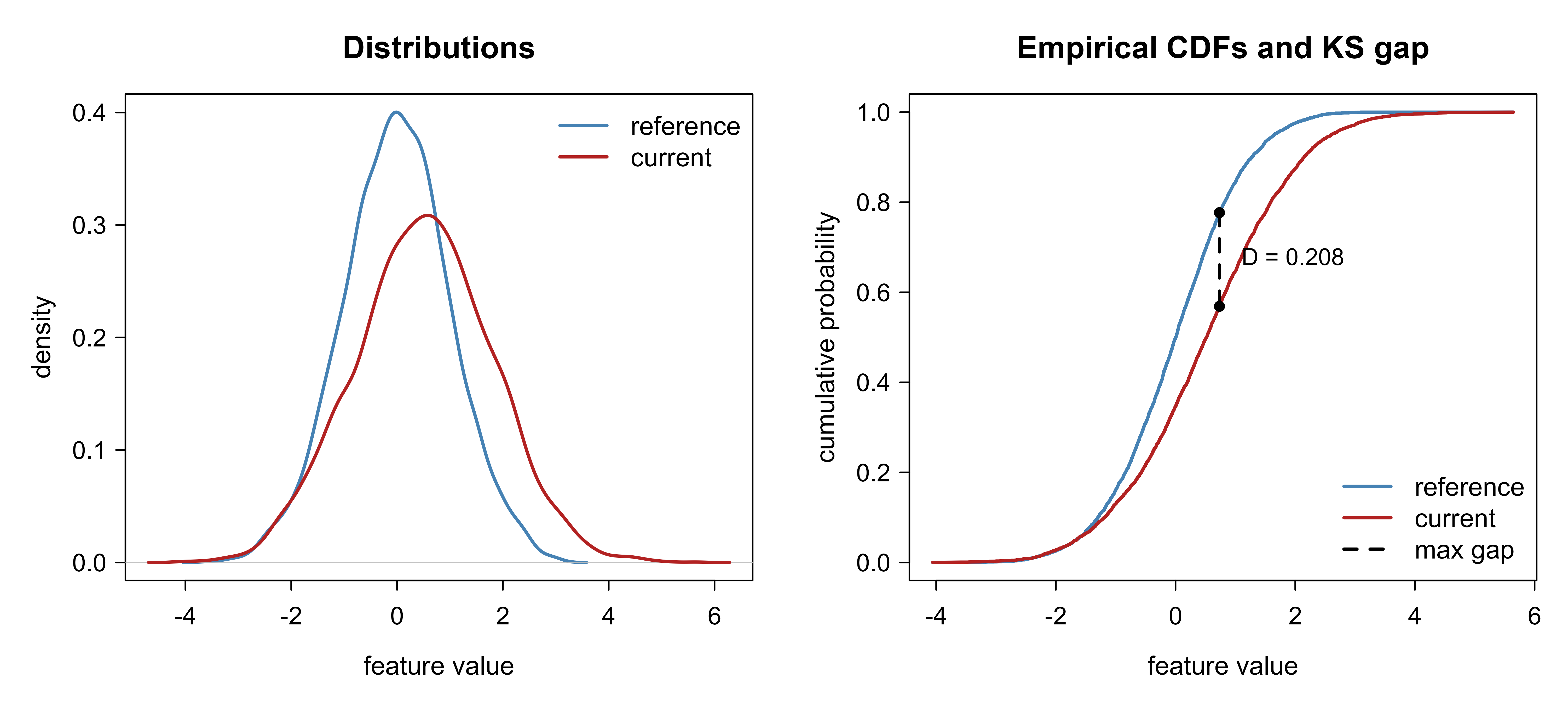
Finally, a tiny simulation that shows how PSI grows as the shift grows, which is the right way to calibrate thresholds for your own data: sweep the mean shift and watch the metric climb past the warn and alert lines. Figure 117.2 traces this relationship.
Show code
shifts <- seq(0, 1.2, by = 0.1)
psi_curve <- sapply(shifts, function(s) {
  cur_s <- rnorm(n_cur, mean = s, sd = 1.0)   # pure location shift
  psi(reference, cur_s, n_bins = 10)$psi
})

plot(shifts, psi_curve, type = "b", pch = 19, col = "darkgreen", lwd = 2,
     xlab = "mean shift of current sample", ylab = "PSI",
     main = "PSI versus magnitude of drift")
abline(h = 0.10, lty = 2, col = "orange")
abline(h = 0.25, lty = 2, col = "red")
text(0.05, 0.11, "warn 0.10", pos = 4, col = "orange", cex = 0.85)
text(0.05, 0.26, "alert 0.25", pos = 4, col = "red", cex = 0.85)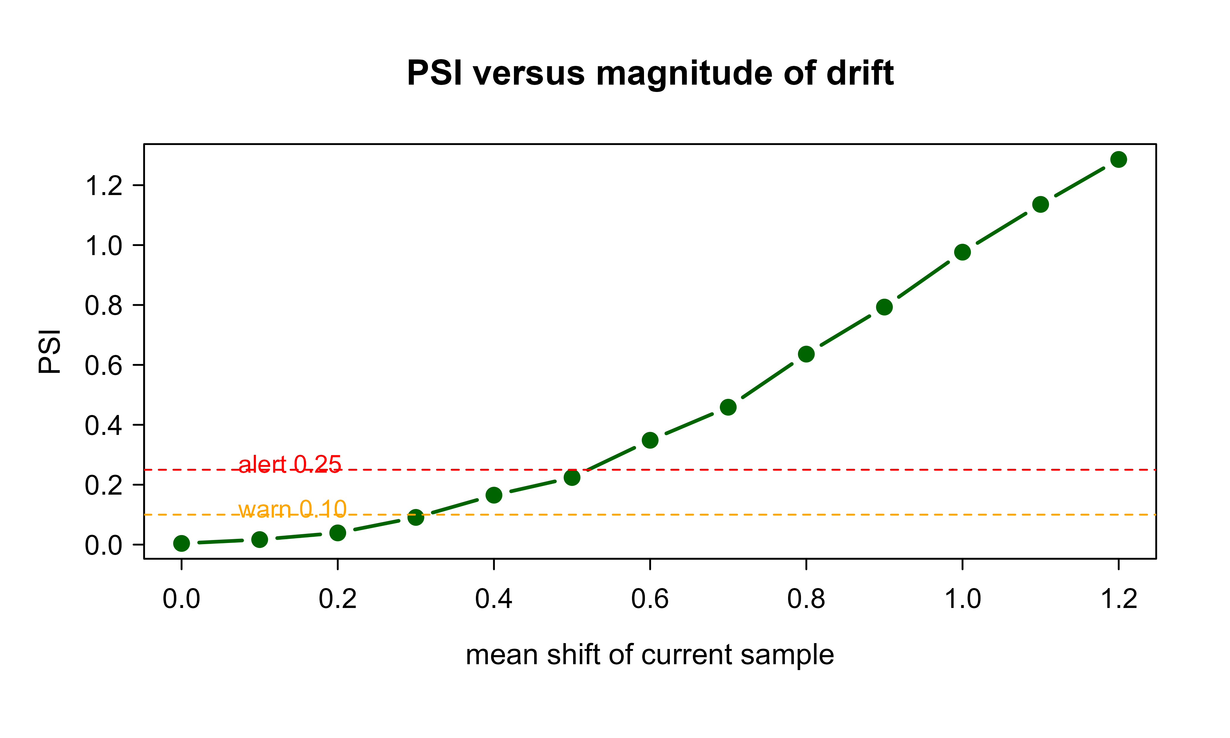
117.6 Performance Monitoring and Retraining Triggers
So far we have watched the inputs. Eventually the labels arrive and we can finally watch the thing we actually care about: whether the model is still right. Distribution metrics are leading indicators; performance metrics are the ground truth, available only once labels arrive. A monitoring program tracks both and uses the cheap label-free signals to decide where to spend scarce labels.
For a classifier, track AUC, log loss, and calibration (Chapter 86) over a sliding or tumbling window.5 For a regressor, track RMSE or MAE and the residual mean (a nonzero residual mean signals systematic bias creeping in). Always track the business metric the model exists to move, because a model can stay statistically accurate while the value it delivers erodes.
Two patterns for windowing, from simplest to most robust:
- Sliding window: compute the metric over the most recent \(w\) scored-and-labeled cases and compare to the validation baseline. Simple, but a single threshold gives no notion of expected fluctuation.
- Control chart: treat the metric as a process and alert when it leaves control limits. If the baseline metric has mean \(\mu_0\) and standard error \(\sigma_0\) (estimated by bootstrapping the validation set or from the window size), alert when the windowed metric \(\theta_t\) satisfies \(|\theta_t - \mu_0| > k\,\sigma_0\), with \(k = 3\) a common choice. This separates real degradation from sampling noise.
Key idea
A single metric crossing a line is not a decision; it might just be noise. The control-chart view asks the better question, “is this change larger than the metric’s normal week-to-week wobble?”, and only then does it alert.
A retraining trigger should combine signals rather than fire on any single metric. A sensible trigger requires several of the following to hold together:
- Sustained performance drop: the windowed metric breaches its control limit for several consecutive windows (not one noisy window).
- Strong, broad input drift: PSI in the alert band on important features, or KS effect sizes that are large (not merely significant), especially on features the model weights heavily.
- Output drift: the predicted-score distribution shifts materially, which often precedes a measured performance drop.
- Enough fresh labeled data exists to retrain on, and the cost of retraining is justified by the expected gain.
Warning
An alert with no owner and no runbook is worse than no alert. People learn to ignore a channel that cries wolf, and then the one alert that mattered gets ignored too. Every threshold you set should answer “who gets paged, and what do they do first?”
Tie the alert to an action and an owner, otherwise alerts become noise that people learn to ignore. The cleanest design routes alerts into the same incident system used for service health, with a runbook: confirm the drift is real (not a pipeline bug or a labeling delay), decide between recalibration and full retraining, and record the decision so the threshold itself can be tuned over time.
117.7 Practical Guidance, Pitfalls, and When to Use What
Use input drift metrics (PSI, KS) whenever labels are delayed or expensive, which is most production settings. They are cheap, run at scoring time, and give the earliest warning. Use output (score) drift as a compact summary when you have many input features: the model’s own score is a learned one-dimensional projection, and a shift in \(P(\hat Y)\) often captures multivariate input drift that no single feature reveals. Use performance metrics (Chapter 82) as the source of truth and as the trigger that actually justifies retraining.
The errors below are the ones that bite teams most often. Each is easy to make and easy to avoid once named:
- Drift is not always decay. \(P(X)\) can move into a region where the model is still accurate. Confirm with performance before retraining; chasing every PSI alert wastes effort and can make things worse if you retrain on a transient blip.
- KS significance is not effect size. At production sample sizes the KS p-value is essentially always below 0.05. Threshold on \(D_{n,m}\) as an effect size, or downsample to a fixed comparison size, rather than reacting to the p-value.
- A fixed reference can go stale. If the reference window is the original training data, slow seasonal drift will eventually flag everything. Decide deliberately whether the reference is the training distribution (detects all change since training) or a recent trailing window (detects sudden change relative to “normal lately”).
- Binning choices change PSI. More bins inflate PSI and add variance in small-mass bins; the \(\epsilon\) floor and the outer \(\pm\infty\) edges matter. Keep the bin definition fixed across time so the metric is comparable.
- Univariate drift misses interactions. Marginals can each look stable while their joint shifts. A model-based check, training a classifier to distinguish reference from current and reading its AUC (the “classifier two-sample test”), catches multivariate drift that per-feature metrics miss.
- Label delay creates blind spots. While labels are pending you are flying on proxies. Document the delay explicitly and size your alerting around it.
- Categorical features need their own treatment. KS is for continuous variables; use PSI on category shares or a chi-square test, and handle new categories that never appeared in the reference.
Tip
The single most useful upgrade to per-feature monitoring is the classifier two-sample test. Pool the reference and current samples, label them by which sample they came from, train any classifier to tell them apart, and read its AUC. An AUC near 0.5 means the two samples are indistinguishable (no drift); an AUC near 1.0 means they are easy to separate (strong, possibly multivariate drift). This catches joint shifts that every marginal misses.
To pull the whole chapter together, here is a reasonable default program: operational health always on; per-feature PSI and KS computed on a daily or weekly batch against a fixed reference, with thresholds calibrated from your own history; score-distribution drift as a single summary; performance metrics on a control chart once labels close; and a combined trigger that requires both a sustained performance signal and corroborating input drift before retraining. The recurring theme is restraint: measure cheaply and often, but act only when independent signals agree.
117.8 Further Reading
- Quionero-Candela, Sugiyama, Schwaighofer, and Lawrence (2009), Dataset Shift in Machine Learning. The standard reference for covariate shift, prior probability shift, and concept shift.
- Gama, Zliobaite, Bifet, Pechenizkiy, and Bouchachia (2014), “A Survey on Concept Drift Adaptation,” ACM Computing Surveys. Broad survey of drift types and adaptation strategies.
- Siddiqi (2006), Credit Risk Scorecards. Origin of the PSI metric and its conventional thresholds in scorecard practice.
- Kolmogorov (1933) and Smirnov (1948). The original two-sample goodness-of-fit statistic and its distribution.
- Lopez-Paz and Oquab (2017), “Revisiting Classifier Two-Sample Tests,” ICLR. The classifier-based approach to multivariate distribution comparison.
- Kullback and Leibler (1951), “On Information and Sufficiency,” Annals of Mathematical Statistics. The divergence underlying PSI.
- Sculley, Holt, Golovin, et al. (2015), “Hidden Technical Debt in Machine Learning Systems,” NeurIPS. Why monitoring and the surrounding plumbing dominate real ML systems.
The statistic is named for Andrey Kolmogorov, who derived the one-sample limiting distribution in 1933, and Nikolai Smirnov, who extended it to the two-sample case in 1948. In monitoring we almost always use the two-sample form, comparing two empirical distributions to each other rather than a sample to a known theoretical law.↩︎
The factorization \(P(X,Y) = P(Y\mid X)\,P(X)\) is just the chain rule of probability; it always holds. Its value here is that it splits the joint distribution into the part a predictive model learns (\(P(Y\mid X)\)) and the part it merely observes as input (\(P(X)\)). Drift can live in either factor, and which factor moved decides what you do about it.↩︎
“Relative entropy” is another name for the Kullback-Leibler divergence, a measure of how different one probability distribution is from another. We make the connection explicit just below; for now read it as “an information-theoretic distance between the reference and current histograms.” Let \(p_b\) be the proportion of the reference sample in bin \(b\) and \(q_b\) the proportion of the current sample in bin \(b\), with \(\sum_b p_b = \sum_b q_b = 1\). Then↩︎
“Nonparametric” means it assumes no particular shape (no normality, no fixed family) for the distributions being compared. It works directly off the empirical distributions, which is exactly what you want in monitoring, where production data rarely follows a tidy textbook distribution.↩︎
A sliding window always covers the last \(w\) cases and moves forward by one each time a new case arrives, so consecutive windows overlap. The same windowing ideas underpin learning on continuously arriving data (Chapter 55). A tumbling window is a fixed, non-overlapping block (for example, each calendar day), so every case belongs to exactly one window. Sliding windows react sooner; tumbling windows are easier to reason about and report.↩︎