| Property | Bare host | Container | Virtual machine |
|---|---|---|---|
| Isolation level | None (shared libraries) | Process + filesystem | Full OS |
| Startup time | Instant | Seconds | Tens of seconds |
| Image / footprint size | n/a | Tens to hundreds of MB | GB |
| Reproducibility | Low (depends on host state) | High (image is fixed) | High (but heavy) |
| Shares host kernel | Yes | Yes | No |
| Typical use | Local dev | Model serving, CI | Strong isolation, mixed OS |
106 Containerizing R and Serving APIs
The API chapter (Chapter 107) shows how to wrap a fitted model behind an HTTP endpoint with plumber. That solves the question of how a model is called. This chapter answers a companion question: how the serving process runs the same way on your laptop, a colleague’s machine, a continuous integration runner, and a production cluster. The answer in current practice is a container: a packaged, isolated, runnable image that carries the R version, the system libraries, the R packages, and your serving code together.
This chapter is about reproducible deployment, not a new estimator. It connects to the API chapter (the thing inside the container is usually a plumber router) and to the chapter on parallel computing (Chapter 95) (the reason you run more than one container).
By the end you will be able to read and write a Dockerfile for an R service, pin package versions so a build today and a build next year behave the same, understand the routing object that lives inside the image, and reason about when adding more containers actually buys you more throughput. None of this requires prior Docker experience; the intuition comes first, and the commands follow.
Intuition
A container is a shipping crate for software. You pack the R runtime, the system libraries, the exact package versions, and your serving code once, seal the crate, and from then on every machine that opens it sees an identical interior. The phrase “it works on my machine” stops being a problem because every machine is now, in effect, your machine.
106.1 Where this fits in a modern ML/AI workflow
A predictive system has a lifecycle: explore, train, evaluate, package, deploy, monitor, retrain. The first half lives in an interactive R session. The second half lives in infrastructure that other systems depend on. The handoff between the two is where most failures happen, and almost all of them have the same shape: “it worked on my machine.”
The phrase hides several distinct problems.
- A different R version evaluates the same code differently (default factor handling, RNG streams,
stringsAsFactors). - A package was updated between training and serving, and a method signature or default changed.
- A system library the package links against (BLAS,
libxml2, GDAL, a CUDA runtime) is missing or a different version. - An environment variable, locale, or file path differs.
A container removes these as variables by shipping all of them inside one artifact. You build an image once (a read-only filesystem snapshot plus metadata about what to run), and every container (a running instance of that image) starts from exactly that snapshot.1 The fitted model, the R runtime, and the plumber code travel together.
Key idea
Each “it worked on my machine” failure is really a hidden dependency that was present on one host and absent on another. Containerization makes every such dependency explicit and ships it along, so there is nothing left to be implicitly different.
The position in the workflow is specific. Containerization happens after you have a serialized model and a serving script, and before the model receives live traffic:
train -> saveRDS(model) -> write plumber.R -> pin package versions -> build image -> run / scale -> monitorEverything in this chapter assumes the modeling work is done. The job here is to make the result portable and identical across environments.
106.2 Containers versus the alternatives
It helps to place containers between two extremes: running directly on a host, and running a full virtual machine. Table 106.1 lays out the three options side by side across the properties that matter for serving.
The container is the middle option that wins for model serving: it is reproducible like a VM but light enough that you can run many replicas of it cheaply, because they all share the host kernel and only carry user-space libraries.2
When to use this
Reach for a container when a model needs to run somewhere other than the laptop it was trained on, especially when other systems or teammates will call it. For a one-off report you will run once and read yourself, a container is more machinery than the job needs.
106.3 A minimal Dockerfile for R
With the conceptual picture in place, we can write the recipe that produces an image. That recipe is a Dockerfile: a plain text file of ordered instructions, read top to bottom, where each instruction adds one layer to the image. For R, the standard base images come from the rocker project, which publishes images such as rocker/r-ver (a fixed R version on Debian) and rocker/r-base (see the Further Reading entry for Boettiger and Eddelbuettel). Pinning the base image tag (writing rocker/r-ver:4.4.3 rather than rocker/r-ver:latest) pins the R version, which is the first reproducibility decision.
Warning
The tag latest is a trap for reproducibility. It means “whatever was newest when you pulled,” so the same Dockerfile can produce different images on different days. Always pin an explicit version tag for anything you intend to rebuild.
Show code
# Dockerfile
# Pin the R version through the base image tag. This fixes the R runtime.
FROM rocker/r-ver:4.4.3

# System libraries that common R packages link against at build/run time.
# Install only what you need; each line adds image size.
RUN apt-get update && apt-get install -y --no-install-recommends \
      libcurl4-openssl-dev \
      libssl-dev \
      libsodium-dev \
    && rm -rf /var/lib/apt/lists/*

# Work inside a known directory.
WORKDIR /app

# Restore the exact package set first, so this layer is cached and only
# rebuilds when the lockfile changes (see the renv section below).
COPY renv.lock renv.lock
RUN R -e "install.packages('renv', repos = 'https://cloud.r-project.org')" \
 && R -e "renv::restore()"

# Copy the serving code and the fitted model artifact.
COPY plumber.R plumber.R
COPY model.rds model.rds

# Document the port the API listens on.
EXPOSE 8000

# Start the API when a container launches.
CMD ["R", "-e", "pr <- plumber::pr('plumber.R'); plumber::pr_run(pr, host = '0.0.0.0', port = 8000)"]
Two ordering choices matter and are easy to get wrong.
- Restore packages before copying code. Docker caches each instruction as a layer. If
renv.lockhas not changed, the expensiverenv::restore()layer is reused, and only the cheapCOPY plumber.Rlayer rebuilds when you edit code. Copying code first would invalidate the package layer on every edit. - Bind to
0.0.0.0, not127.0.0.1. Inside a container,127.0.0.1is the container’s own loopback, unreachable from the host. Listening on0.0.0.0accepts connections forwarded from outside.
Building and running use the shell, not R:
Show code
# Build an image and tag it.
docker build -t my-model-api:1.0 .

# Run a container, mapping host port 8000 to container port 8000.
docker run --rm -p 8000:8000 my-model-api:1.0

# From another terminal, call the running API.
curl -X POST "http://localhost:8000/predict" \
  -H "Content-Type: application/json" \
  -d '{"sepal_length":5.1,"sepal_width":3.5,"petal_length":1.4,"petal_width":0.2}'
106.4 Pinning package versions with renv
Pinning the base image solved the R version, but it left a gap: the packages your model depends on are still unpinned. A fixed base image fixes R but not the packages. Without a lockfile, install.packages("xgboost") installs whatever is current on the day you build, which drifts over time. The renv package solves this by recording the exact version (and source) of every package in a renv.lock file, then restoring that exact set later.3
The mental model is a function. Let \(P\) be the set of packages your project loads, and for each package \(p \in P\) let \(v(p)\) be its installed version. The lockfile stores the pair set
\[ L = \{ (p, v(p)) : p \in P \}, \]
and renv::restore() is the operation that reconstructs an environment whose installed versions match \(L\) exactly. Reproducibility is the statement that building from the same \((\text{base image}, L)\) on any host yields the same serving behavior.
The workflow during development:
Show code
# Once, in your project:
renv::init()      # create a project-private library and the first renv.lock

# After installing or upgrading packages you depend on:
renv::snapshot()  # write the current versions into renv.lock

# Anywhere later (including inside the Dockerfile):
renv::restore()   # install exactly the versions recorded in renv.lock
renv records not only versions but the repository snapshot (for example a Posit Public Package Manager URL dated to a specific day), so even a package that was later removed from CRAN can still be reinstalled. Commit renv.lock to version control; it is the single source of truth for the environment.
Tip
Treat renv.lock the way you treat your source code: commit it, review changes to it, and rebuild the image whenever it changes. A lockfile that lives only on one developer’s laptop reproduces nothing.
Table 106.2 separates what each layer pins, which is the clearest way to see why you need all three.
| Layer | Pins | Without it |
|---|---|---|
| Base image tag | R version + OS | R behavior drifts across builds |
| System libs (apt) | C/C++ shared libraries | Packages fail to load or link |
| renv.lock | R package versions | Package APIs drift across builds |
106.5 What the container serves: a plumber router
We have built and pinned the image; now we open the crate and look at what runs inside. Inside the image, the served object is a plumber router: an R object that maps HTTP method and path pairs to handler functions.4 The API chapter covers the annotated-comment style (#* @post /predict). You can also build the same router programmatically, which is convenient for understanding what the object is and for testing it without opening a socket.
The following chunk is runnable. It constructs a router and registers two routes, then inspects the object. It does not call pr_run(), so no server starts and no port is opened; we only build and examine the routing table. The plumber package may not be installed in every environment, so the demo is written to degrade to a plain-R stand-in if plumber is absent, which keeps the teaching point (a router is a lookup table from routes to handlers) intact.
Show code
have_plumber <- requireNamespace("plumber", quietly = TRUE)

# The two handlers our API exposes.
health_handler <- function() list(status = "ok")

predict_handler <- function(sepal_length, sepal_width,
                            petal_length, petal_width) {
  # A stand-in "model": a fixed linear score. In production this would be
  # predict(model, newdata). The point here is the request-to-response shape.
  x <- c(as.numeric(sepal_length), as.numeric(sepal_width),
         as.numeric(petal_length), as.numeric(petal_width))
  beta <- c(0.2, -0.1, 0.4, 0.3)
  list(prediction = as.numeric(crossprod(beta, x)))
}

if (have_plumber) {
  pr <- plumber::pr()
  pr <- plumber::pr_get(pr, "/health", health_handler)
  pr <- plumber::pr_post(pr, "/predict", predict_handler)
  # Inspect the router's registered endpoints without serving.
  routes <- vapply(pr$endpoints[[1]], function(e) {
    paste(paste(e$verbs, collapse = ","), e$path)
  }, character(1))
  cat("plumber router endpoints:\n"); print(routes)
} else {
  # Plain-R stand-in: a router is just a named lookup of (verb, path) -> handler.
  router <- list(
    `GET /health`   = health_handler,
    `POST /predict` = predict_handler
  )
  cat("router endpoints (plain-R stand-in):\n"); print(names(router))
}
#> plumber router endpoints:
#> [1] "GET /health"   "POST /predict"
Either way the object is the same idea: a finite set of routes, each route a (verb, path) key pointing at a function that maps parsed inputs to a serializable list.
106.6 A base-R request/response simulation
The router told us what the server holds. To see what it does with each incoming request, without Docker, sockets, or a network, we can simulate the request/response cycle in base R. A request is a method, a path, and a parsed body; the server dispatches on (method, path), runs the handler, and serializes the returned list to a JSON-like string. This is exactly the loop plumber runs, stripped to its logic.
Note
The to_json function below is a deliberately tiny serializer for teaching only. It handles flat named lists of scalars and nothing more. Real serving uses jsonlite, which plumber calls for you and which handles nesting, vectors, and edge cases the toy version ignores.
Show code
# A tiny router: named list keyed by "VERB /path".
router <- list(
  `GET /health`   = health_handler,
  `POST /predict` = predict_handler
)

# Minimal JSON serializer for flat named lists of scalars (teaching only).
to_json <- function(x) {
  parts <- vapply(names(x), function(nm) {
    v <- x[[nm]]
    val <- if (is.character(v)) paste0("\"", v, "\"") else format(v, digits = 6)
    paste0("\"", nm, "\":", val)
  }, character(1))
  paste0("{", paste(parts, collapse = ","), "}")
}

# The server loop: dispatch one request to its handler and serialize.
serve <- function(method, path, body = list()) {
  key <- paste(method, path)
  handler <- router[[key]]
  if (is.null(handler)) {
    return(list(status = 404L, body = to_json(list(error = "not found"))))
  }
  result <- tryCatch(
    do.call(handler, body),
    error = function(e) list(error = conditionMessage(e))
  )
  status <- if (!is.null(result$error)) 400L else 200L
  list(status = status, body = to_json(result))
}

# Simulate three incoming requests.
req1 <- serve("GET",  "/health")
req2 <- serve("POST", "/predict",
              body = list(sepal_length = 5.1, sepal_width = 3.5,
                          petal_length = 1.4, petal_width = 0.2))
req3 <- serve("POST", "/unknown")

cat("GET  /health ->", req1$status, req1$body, "\n")
#> GET  /health -> 200 {"status":"ok"}
cat("POST /predict ->", req2$status, req2$body, "\n")
#> POST /predict -> 200 {"prediction":1.29}
cat("POST /unknown ->", req3$status, req3$body, "\n")
#> POST /unknown -> 404 {"error":"not found"}
The simulation makes three production facts concrete: dispatch is a table lookup, unknown routes must return a 404 rather than crash, and a handler error should become a 400 response rather than take the server down.
106.7 A figure: why replicas, and how throughput scales
So far the focus has been reproducibility: making one container behave the same everywhere. The other half of the payoff is scaling. Because identical images are trivial to replicate behind a load balancer, you can answer more traffic simply by running more copies. A single R process is largely single-threaded for request handling, so it serves roughly one request at a time. If each request takes a fixed service time, then running \(k\) identical container replicas multiplies the throughput ceiling by \(k\) (up to the point where a shared resource, the database, the host CPU, or the network, saturates).
A simple model: let \(s\) be the mean service time per request in seconds. One replica can sustain about \(1/s\) requests per second; \(k\) replicas sustain about \(k/s\), until a hard ceiling \(C\) imposed by a shared bottleneck. The achievable throughput is
\[ T(k) = \min\!\left(\frac{k}{s},\, C\right). \]
Figure 106.1 plots \(T(k)\) for a representative service time and ceiling. The linear region is where adding replicas helps; the flat region is where you have hit a shared limit and more containers stop paying off.
Intuition
Adding replicas is like opening more checkout lanes. More lanes clear the queue faster, right up until the single shared exit door (the database, the host CPU) becomes the line everyone waits in. Past that point, new lanes serve no one.
Show code
library(ggplot2)

s <- 0.05          # mean service time per request, seconds (20 req/s per replica)
C <- 250           # shared bottleneck ceiling, requests/second
k <- 1:24
throughput <- pmin(k / s, C)

df <- data.frame(replicas = k, throughput = throughput)
knee <- ceiling(C * s)   # replica count where the ceiling is first hit

ggplot(df, aes(replicas, throughput)) +
  geom_line(color = "#2c7fb8", linewidth = 1) +
  geom_point(color = "#2c7fb8") +
  geom_hline(yintercept = C, linetype = "dashed", color = "grey40") +
  geom_vline(xintercept = knee, linetype = "dotted", color = "grey40") +
  annotate("text", x = max(k), y = C, label = "shared ceiling C",
           hjust = 1, vjust = -0.6, size = 3.3, color = "grey30") +
  labs(x = "container replicas (k)",
       y = "sustainable throughput (requests / second)",
       title = "Replicas help until a shared resource saturates") +
  theme_minimal(base_size = 12)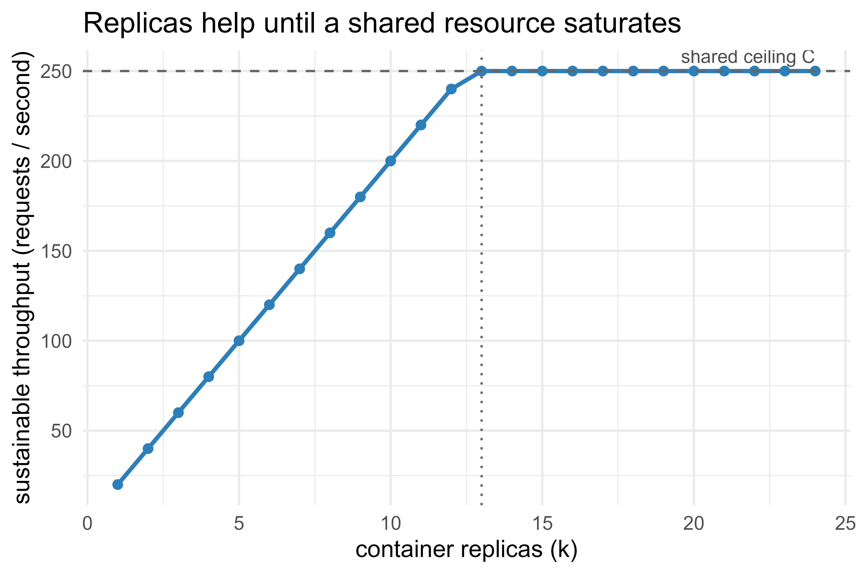
The practical reading: containers make horizontal scaling cheap, but throughput is not free past the knee. Before adding replicas, confirm the bottleneck is the R process and not a downstream database or the host’s CPU.
106.8 Orchestrating multiple containers with docker-compose
The \(T(k)\) curve assumed something would route requests across the replicas. That router, plus everything else a real deployment needs, is what we wire up next. Real services rarely run alone. A typical stack is the model API plus a reverse proxy (and perhaps a cache or a database).5 docker-compose describes a multi-container application declaratively in one file, so the whole stack starts with one command.
Show code
# docker-compose.yml
services:
  api:
    build: .
    expose:
      - "8000"
    deploy:
      replicas: 3          # run three identical API containers
    environment:
      - R_KEEP_PKG_SOURCE=no
    restart: unless-stopped

  proxy:
    image: nginx:1.27
    ports:
      - "80:80"            # public entrypoint
    volumes:
      - ./nginx.conf:/etc/nginx/conf.d/default.conf:ro
    depends_on:
      - api
Show code
# Build images and start the whole stack in the background.
docker compose up --build -d

# Scale the API service up or down at runtime.
docker compose up -d --scale api=5

# Tear everything down.
docker compose down
The proxy (here nginx) load-balances across the API replicas, which is the practical realization of the \(T(k)\) curve above. The same description runs identically on a developer laptop and a single production host; for larger clusters the same images move to an orchestrator such as Kubernetes with little change to the image itself.
106.9 Practical guidance, pitfalls, and when to use it
When containerizing R is worth it:
- The model will be called by other systems or other people, not just you.
- Reproducibility across machines matters (regulated settings, audits, team handoffs).
- You need to scale horizontally or deploy to a cluster.
When it is overkill:
- A one-off analysis or a report. A pinned
renvproject is enough; you do not need an image. - A purely interactive workflow where you are the only consumer.
Common pitfalls, most of which cost hours the first time:
- Forgetting to bind
0.0.0.0. The API runs but is unreachable from the host. Always sethost = "0.0.0.0"inpr_run(). - No lockfile. A pinned base image with unpinned packages is only half reproducible; the build silently changes over time. Commit
renv.lock. - Fat images. Installing build toolchains and dev headers you only need at build time bloats the image and widens the attack surface. Use
--no-install-recommends, cleanaptlists, and consider multi-stage builds that compile in one stage and copy only artifacts into a slim final stage. - Loading the model per request. Load
model.rdsonce at startup (top ofplumber.R), not inside the handler. Per-request loading dominates latency. - No input validation. A container does not validate inputs for you. Check types, ranges, and required fields in the handler and return
400on bad input, as the simulation showed. - Running as root. The default container user is
root. Create and switch to a non-root user (USER) for anything exposed to a network. - Treating the image as mutable. Do not exec into a running container and patch it. Change the
Dockerfileor lockfile, rebuild, and redeploy, so the artifact stays the source of truth.
Warning
The single most common security mistake here is leaving the container running as root while it is exposed to a network. If the serving process is compromised, an attacker inherits whatever the container user can do. Add a USER instruction to drop to an unprivileged account before the CMD runs.
For production model lifecycle (versioning, automatic Dockerfile generation, deployment to a board, and drift monitoring), vetiver builds directly on plumber and pins and is the natural next step; see the API chapter’s (Chapter 107) discussion of versioning and hosting, the model deployment chapter (Chapter 116) for serving patterns, and the model monitoring chapter (Chapter 117) for drift detection.
To recap the path through the chapter: a container packages the R runtime, system libraries, pinned packages, and serving code into one portable artifact; a Dockerfile is the recipe and renv.lock pins the package layer; inside the image a plumber router dispatches requests to handler functions, exactly as the base-R simulation made concrete; and identical images replicate cheaply behind a proxy, which buys throughput up to the first shared bottleneck. With those pieces, the handoff from “it trains in my session” to “it serves the same way everywhere” stops being the place where deployments break.
106.10 Further reading
- Boettiger, C. and Eddelbuettel, D. (2017). “An Introduction to Rocker: Docker Containers for R.” The R Journal.
- Nüst, D. et al. (2020). “Ten simple rules for writing Dockerfiles for reproducible data science.” PLOS Computational Biology.
- Ushey, K. and Wickham, H.
renvdocumentation: https://rstudio.github.io/renv/. - Schloerke, B. and Allen, J.
plumberdocumentation: https://www.rplumber.io/. - The Rocker Project: https://rocker-project.org/.
- Docker documentation, “Best practices for writing Dockerfiles”: https://docs.docker.com/develop/develop-images/dockerfile_best-practices/.
- Vaughan, D. and Silge, J.
vetiverdocumentation: https://rstudio.github.io/vetiver-r/.
The image-versus-container distinction is the one piece of vocabulary worth fixing early. An image is the recipe plus the frozen ingredients; a container is a meal cooked from it. One image can spawn many containers, and they cannot drift apart because they all start from the same read-only layers.↩︎
Sharing the host kernel is exactly why a container starts in seconds while a virtual machine boots a whole operating system. The trade-off is that a container is not as strongly isolated as a VM, which matters when you must run untrusted code or a different operating system entirely. For serving your own R model, that weaker isolation is a fair price for the speed and small footprint.↩︎
The name is short for “reproducible environment.” It works by giving each project its own private package library, isolated from your system-wide library, so projects cannot quietly share or overwrite each other’s package versions.↩︎
A handler is just an ordinary R function. The router’s only job is to decide which handler to call for an incoming request, then hand that function the parsed inputs and serialize whatever it returns. There is no magic; it is a lookup table wrapped around a web server.↩︎
A reverse proxy is a server that sits in front of your API containers and forwards each incoming request to one of them. Besides spreading load, it gives you a single public address, a place to terminate TLS, and a natural spot for rate limiting.↩︎