98  Automated Machine Learning (AutoML)

Suppose a colleague drops a clean tabular dataset on your desk and asks for the best predictive model you can build by tomorrow morning. A practiced data scientist runs the same loop every time: try a penalized linear model, a couple of tree ensembles, maybe a small neural network; tune each one’s knobs; decide how to encode the categorical columns and what to do about missing values; compare everything honestly on held-out data; and ship the winner. The loop is mechanical enough that you could almost write it down as an algorithm. Automated Machine Learning (AutoML) is the attempt to do exactly that: turn the search over preprocessing, model family, and hyperparameters into an optimization problem that a computer can solve while you sleep.

The promise is appealing and the danger is real, so it is worth being precise about what AutoML actually optimizes. It does not invent new model families or discover causal structure. It searches a space you defined, using a budget you set, to minimize an estimate of generalization error you chose. Everything good and everything bad about AutoML follows from that one sentence. The good: it explores far more combinations than a human would, without fatigue or favoritism toward the method you happen to know best. The bad: if the search space is wrong, the budget is too small, or the error estimate is optimistic, AutoML will confidently hand you a model that looks excellent on your validation data and disappoints in production.

This chapter develops the idea from the ground up. We start with the central formalism, the Combined Algorithm Selection and Hyperparameter optimization (CASH) problem, which unifies “which model” and “which settings” into a single objective. We then look at how that objective is actually searched (random search, Bayesian optimization, and a brief note on neural architecture search), how meta-learning lets a system warm-start from past experience instead of starting cold, and how the major tools (h2o AutoML and auto-sklearn) put the pieces together. A runnable base-R demonstration builds a miniature AutoML system that searches over several model families with nested cross-validation and reports a leaderboard, so the mechanics are concrete rather than magical. We close with the pitfalls that separate a useful AutoML run from a misleading one. This chapter leans on the hyperparameter optimization chapter (Chapter 84) for the inner search and on the feature engineering chapter (Chapter 83) for the preprocessing pieces; AutoML is, in a sense, those two chapters wrapped in an outer loop together with model selection.

Note

A companion chapter on scalable machine learning with h2o (Chapter 97) covers the h2o.automl() interface and a base-R leaderboard at the engine level. This chapter is the conceptual counterpart: what AutoML is optimizing, how the search works, and why it can mislead. The two are meant to be read together.

98.1 The pipeline AutoML automates

Before formalizing anything, it helps to name the parts. A supervised learning pipeline is a function from raw data to predictions, built by composing a few stages. AutoML systems differ in how many of these stages they automate, but the menu is always some subset of the following.

• Feature preprocessing. Imputation of missing values, encoding of categorical variables, scaling of numeric columns, and optional feature construction or selection. This is the subject of the feature engineering chapter (Chapter 83); AutoML treats the choices there (which imputer, which encoder) as decisions to be searched, not fixed in advance.
• Model selection. Choosing the learning algorithm itself: elastic-net GLM, random forest, gradient boosting, k-nearest neighbors, a small neural network, and so on. Each is a different inductive bias, and which one fits best is data-dependent.
• Hyperparameter optimization. Tuning the continuous and discrete knobs of whichever model is selected: the penalty \(\lambda\) of a GLM, the depth and learning rate of a booster, the number of neighbors \(k\). This is the subject of the hyperparameter optimization chapter (Chapter 84).
• Ensembling. Combining several trained models, usually by stacking, so the final prediction is better than any single member.
• Neural architecture search (NAS). When the model family is a neural network, the architecture itself (depth, width, connectivity) becomes a hyperparameter. We treat this briefly because it is computationally heavy and largely separate from tabular AutoML.

Key idea

AutoML is not one algorithm. It is an outer optimization loop that treats the choice of preprocessing, model, and hyperparameters as a single joint decision, scored by an estimate of generalization error.

The reason these stages cannot be optimized independently is interaction. The best learning rate for a booster depends on its depth; the best model family depends on how the features were encoded; whether to standardize depends on whether the model is distance-based (k-nearest neighbors cares, trees do not). Optimizing each stage in isolation and gluing the winners together can produce a pipeline that no stage would have chosen jointly. The next section makes this joint view precise.

98.2 The CASH problem

The formalism that organizes AutoML is the Combined Algorithm Selection and Hyperparameter optimization problem, introduced by Thornton, Hutter, Hoos, and Leyton-Brown (2013). The name is a mouthful but the idea is clean: stop treating “pick a model” and “tune it” as two steps, and treat them as one search over a single combined space.

Let \(\mathcal{A} = \{A^{(1)}, A^{(2)}, \dots, A^{(R)}\}\) be a set of candidate learning algorithms (the model families plus, in full generality, the preprocessing operators). Each algorithm \(A^{(j)}\) has its own hyperparameter space \(\Lambda^{(j)}\), which may be continuous (a learning rate), integer (a tree depth), or categorical (a kernel type), and may itself be conditional: a parameter exists only when another takes a certain value.¹ A single point in the combined space is a pair \((A^{(j)}, \boldsymbol\lambda)\) with \(\boldsymbol\lambda \in \Lambda^{(j)}\): a choice of algorithm together with a full setting of its knobs.

Given a dataset \(\mathcal{D}\) split into \(K\) cross-validation folds \(\mathcal{D} = \mathcal{D}^{(1)} \cup \cdots \cup \mathcal{D}^{(K)}\), write \(\mathcal{L}\big(A^{(j)}_{\boldsymbol\lambda}, \mathcal{D}_{\text{train}}, \mathcal{D}_{\text{valid}}\big)\) for the loss (misclassification rate, RMSE, deviance, whatever you chose) obtained when algorithm \(A^{(j)}\) with hyperparameters \(\boldsymbol\lambda\) is trained on \(\mathcal{D}_{\text{train}}\) and scored on \(\mathcal{D}_{\text{valid}}\). The CASH problem is to find the algorithm-and-hyperparameter pair that minimizes the cross-validated loss:

\[ (A^{\star}, \boldsymbol\lambda^{\star}) \;=\; \operatorname*{arg\,min}_{A^{(j)} \in \mathcal{A},\; \boldsymbol\lambda \in \Lambda^{(j)}} \; \frac{1}{K} \sum_{k=1}^{K} \mathcal{L}\Big(A^{(j)}_{\boldsymbol\lambda}, \, \mathcal{D} \setminus \mathcal{D}^{(k)}, \, \mathcal{D}^{(k)}\Big). \]

Read it slowly. The inner part is exactly the \(K\)-fold cross-validation estimate of generalization error for one fixed pipeline. The outer \(\arg\min\) ranges over every algorithm and every legal hyperparameter setting at once. That single \(\arg\min\) over a union of heterogeneous spaces is what makes CASH the right abstraction: it refuses to separate “which model” from “which settings,” because the best settings depend on the model and the best model depends on its settings.

Intuition

Picture a vast, lumpy landscape whose horizontal coordinates are “which algorithm” and “what hyperparameters,” and whose height is cross-validated error. The landscape is not even connected in a simple way: moving from the random-forest region to the GLM region crosses a boundary where the very meaning of the coordinates changes. CASH asks for the lowest point in this whole strange landscape, and AutoML is the machinery for searching it without evaluating every point.

One trick collapses the union of spaces into a single space, which is how tools implement CASH in practice. Introduce a top-level categorical hyperparameter \(\theta\) whose value names the chosen algorithm, so \(\theta \in \{1, \dots, R\}\), and make every algorithm-specific parameter conditional on \(\theta\). Then the combined space is one (structured, conditional) hyperparameter space

\[ \Lambda \;=\; \{\theta\} \,\cup\, \Lambda^{(1)} \cup \cdots \cup \Lambda^{(R)}, \]

and CASH becomes an ordinary, if high-dimensional and conditional, hyperparameter optimization problem over \(\Lambda\). This is precisely why the same optimizers used for hyperparameter tuning (random search, Bayesian optimization) apply directly to model selection: once you write model choice as a hyperparameter, selecting a model is just tuning \(\theta\).

Warning

The objective above minimizes cross-validated loss, which is an estimate of generalization error, not the truth. Search hard enough over enough pipelines and you will find one whose cross-validation score is low partly by luck. This is overfitting the validation procedure itself, and it is the defining hazard of AutoML. We return to it in the pitfalls section, and the demonstration measures it directly.

98.3 Searching the CASH space

The CASH objective tells us what to minimize; it says nothing about how. Every entry on the right-hand side requires training a full model, which can take seconds to hours, so the search must be sample-efficient: find a good pipeline in as few evaluations as the budget allows. Three approaches dominate, in increasing sophistication.

98.3.1 Grid and random search

The simplest strategy fixes a finite list of pipelines and evaluates them all. Grid search lays a regular lattice over each hyperparameter; random search draws each configuration independently from a distribution over \(\Lambda\). Bergstra and Bengio (2012) showed that random search is usually the better of the two for the same budget, and the reason is geometric. If only a few of the hyperparameters actually matter (the common case), a grid wastes its budget by repeatedly testing the irrelevant ones at the same few values, whereas random search gives every important dimension many distinct values for the same number of trials.

Intuition

Imagine tuning two knobs where only one affects performance. A \(5 \times 5\) grid tests the important knob at just 5 distinct settings (25 runs total). Twenty-five random draws test it at 25 distinct settings. Same cost, five times the resolution where it counts.

Random search is the honest baseline for any AutoML claim. It is trivial to parallelize (every trial is independent), it has no failure modes beyond the budget, and a more clever method that cannot beat random search is not worth its complexity. Its weakness is that it never learns: trial 100 is drawn the same way as trial 1, ignoring everything the first 99 revealed.

98.3.2 Bayesian optimization

Bayesian optimization (BO) fixes that weakness by building a probabilistic model of the objective and using it to decide where to evaluate next. Treat the cross-validated loss as an unknown function \(f(\boldsymbol\lambda)\) that is expensive to query. After observing trials \(\mathcal{H}_t = \{(\boldsymbol\lambda_1, y_1), \dots, (\boldsymbol\lambda_t, y_t)\}\) with \(y_i = f(\boldsymbol\lambda_i)\), fit a surrogate model that gives, for any candidate \(\boldsymbol\lambda\), a predicted mean \(\mu_t(\boldsymbol\lambda)\) and uncertainty \(\sigma_t(\boldsymbol\lambda)\). An acquisition function then scores candidates by trading off exploitation (low predicted loss) against exploration (high uncertainty), and the next trial is its maximizer:

\[ \boldsymbol\lambda_{t+1} \;=\; \operatorname*{arg\,max}_{\boldsymbol\lambda \in \Lambda} \; a\big(\boldsymbol\lambda \mid \mathcal{H}_t\big). \]

A common acquisition function is Expected Improvement. With \(f^{\star}_t = \min_{i \le t} y_i\) the best loss seen so far, and treating the surrogate’s prediction at \(\boldsymbol\lambda\) as Gaussian with mean \(\mu_t\) and standard deviation \(\sigma_t\), the expected improvement over the incumbent is

\[ \operatorname{EI}(\boldsymbol\lambda) \;=\; \mathbb{E}\big[\max\big(f^{\star}_t - f(\boldsymbol\lambda),\, 0\big)\big] \;=\; \big(f^{\star}_t - \mu_t(\boldsymbol\lambda)\big)\,\Phi(z) + \sigma_t(\boldsymbol\lambda)\,\phi(z), \qquad z = \frac{f^{\star}_t - \mu_t(\boldsymbol\lambda)}{\sigma_t(\boldsymbol\lambda)}, \]

where \(\Phi\) and \(\phi\) are the standard normal CDF and PDF. The first term rewards candidates predicted to beat the incumbent; the second rewards uncertain candidates, since a wide \(\sigma_t\) means a real chance of a large improvement. Maximizing EI is cheap because it only queries the surrogate, not the true expensive objective.

The choice of surrogate matters for AutoML specifically. A Gaussian process is the textbook choice but struggles with the conditional, partly-categorical CASH space (the \(\theta\) that selects the algorithm). For that reason, the influential auto-sklearn and Auto-WEKA systems use a random-forest surrogate (the SMAC method of Hutter, Hoos, and Leyton-Brown, 2011), which handles categorical and conditional dimensions naturally. Tree-structured Parzen estimators (Bergstra et al., 2011) are another popular surrogate that models \(p(\boldsymbol\lambda \mid y)\) rather than \(p(y \mid \boldsymbol\lambda)\).

Key idea

Bayesian optimization spends a little computation deciding where to look so it can spend far less computation looking. It pays off when each evaluation (each model fit) is expensive relative to fitting the surrogate, which is exactly the AutoML regime.

98.3.3 Neural architecture search, briefly

When the model is a neural network, the architecture (how many layers, how wide, which connections) is itself part of \(\boldsymbol\lambda\), and searching over architectures is called neural architecture search. The combined space is enormous and each evaluation trains a network, so naive NAS can cost thousands of GPU-days. The field’s progress is mostly about making the search cheaper: weight sharing across candidate architectures (ENAS), continuous relaxations that make the architecture differentiable (DARTS, Liu et al., 2019), and predicting a network’s final accuracy from a few epochs. NAS matters for images, text, and other domains where architecture is decisive. For the tabular problems most AutoML systems target, a well-tuned gradient boosting machine usually beats a searched network at a fraction of the cost, so we mention NAS for completeness and spend our runnable budget elsewhere.

When to use this

Reach for NAS only when the architecture is genuinely the bottleneck (large-scale vision or language) and you have the compute to match. For tabular data, put the budget into searching model families and their hyperparameters, not into discovering a custom network.

98.4 Meta-learning and warm-starting

Everything so far starts each new dataset from scratch, as if no model had ever been fit to any data before. That is wasteful. A human expert facing a new tabular problem does not begin by trying random hyperparameters; they begin near settings that worked on similar problems in the past. Meta-learning is the machinery that gives an AutoML system the same head start.

The setup is to learn across datasets. Suppose you have a collection of past datasets \(\mathcal{D}_1, \dots, \mathcal{D}_M\), and for each you recorded its meta-features \(\mathbf{m}_i \in \mathbb{R}^d\) (number of rows, number of features, fraction missing, class imbalance, simple landmarking scores from fast models) together with the configuration \(\boldsymbol\lambda_i^{\star}\) that worked best on it. Given a new dataset with meta-features \(\mathbf{m}_{\text{new}}\), the meta-learner finds the past datasets most similar to it,

\[ \mathcal{N}(\mathbf{m}_{\text{new}}) \;=\; \big\{\, i : \lVert \mathbf{m}_i - \mathbf{m}_{\text{new}} \rVert \text{ is among the } L \text{ smallest} \,\big\}, \]

and seeds the search with their winning configurations \(\{\boldsymbol\lambda_i^{\star} : i \in \mathcal{N}(\mathbf{m}_{\text{new}})\}\) instead of random points. This is warm-starting: the optimizer’s first few trials are educated guesses drawn from experience, so it spends its budget refining good regions rather than discovering them.

Intuition

Meta-learning is the AutoML system’s memory. The first time it sees a wide, sparse, imbalanced dataset it has to search blindly; the hundredth time, it recognizes the type and starts where similar datasets ended up. The similarity is measured in meta-feature space, not in the raw data.

The auto-sklearn system of Feurer et al. (2015) is the canonical example: it precomputed the best configurations on a large bank of OpenML datasets, and at runtime it uses meta-features to pick a handful of those configurations to initialize Bayesian optimization. The reported effect is that the search reaches a good model much earlier in its budget, which matters most when the budget is short. A second, related technique those systems use is post-hoc ensembling: rather than keep only the single best pipeline the search found, build a weighted ensemble from the many pipelines it trained along the way, which are otherwise discarded. The leaderboard the search produces is, conveniently, exactly the pool an ensemble selection method (Caruana et al., 2004) draws from.

98.5 Tools in practice

Two open systems anchor the practical landscape, and they make different design choices worth contrasting. Table 98.1 summarizes them alongside the base-R demonstration built later in this chapter, so the moving parts of each are visible side by side.

Table 98.1: Design choices of two production AutoML systems and the base-R demonstration in this chapter, compared across search strategy, surrogate, meta-learning, the form of the final model, the model families considered, native R access, and intended use.

Aspect	h2o AutoML	auto-sklearn	This chapter’s demo
Search strategy	Random search over a fixed plan	Bayesian optimization (SMAC)	Exhaustive grid (CASH)
Surrogate model	None (predefined grid + RS)	Random forest (SMAC)	None (full enumeration)
Meta-learning / warm-start	No (fixed search plan)	Yes (meta-features + OpenML bank)	No
Final model	Stacked ensemble (default leader)	Ensemble selection over trials	Best pipeline + stacked ensemble
Model families	GLM, GBM, RF, XRT, deep net	scikit-learn estimators + preprocessors	GLM, elastic net, kNN, tree
Native R access	Yes (h2o package)	No (Python)	Yes (base R)
Typical use	Strong tabular baseline from one call	Sample-efficient search under a budget	Teaching the CASH mechanics

Table 98.1 draws out the main contrast. h2o AutoML follows a fixed, mostly random search plan and always finishes by training a stacked ensemble, which makes it a one-call workhorse for a strong tabular baseline and is covered in detail in the h2o chapter (Chapter 97). auto-sklearn instead spends effort on a Bayesian-optimization search seeded by meta-learning and finishes with post-hoc ensemble selection, which makes it more sample-efficient under a tight budget at the cost of more machinery. The base-R demonstration below strips both down to the bones: it enumerates the CASH grid exactly so you can see the objective being minimized with nothing hidden.

The h2o call is shown for reference (it needs a running JVM cluster, so it does not execute when the book is built):

library(h2o)
h2o.init(nthreads = -1, max_mem_size = "4G")

train_h2o <- as.h2o(train_df)
train_h2o[["y"]] <- as.factor(train_h2o[["y"]])   # classification needs a factor
x <- setdiff(colnames(train_h2o), "y")

aml <- h2o.automl(
  x = x, y = "y", training_frame = train_h2o,
  max_runtime_secs = 300,   # the budget; or use max_models
  nfolds = 5,
  sort_metric = "AUC",
  seed = 1
)
h2o.get_leaderboard(aml, extra_columns = "ALL")   # the ranked pipelines
best <- aml@leader                                # usually a stacked ensemble
h2o.shutdown(prompt = FALSE)

The auto-sklearn call is Python (no native R interface), shown so the API parallel is clear:

import autosklearn.classification

automl = autosklearn.classification.AutoSklearnClassifier(
    time_left_for_this_task=300,      # the budget, in seconds
    per_run_time_limit=30,
    metric=autosklearn.metrics.roc_auc,
    ensemble_size=50,                 # post-hoc ensemble selection
)
automl.fit(X_train, y_train)
print(automl.leaderboard())           # the ranked pipelines
print(automl.show_models())           # the ensemble it kept

98.6 A runnable demonstration: a miniature AutoML system

The fastest way to demystify AutoML is to build one small enough to read in full. The demonstration below implements the CASH problem directly in base R. It defines a search space of four model families with a few hyperparameter settings each, estimates each pipeline’s generalization error with cross-validation, ranks them on a leaderboard, and then does the one thing a leaderboard alone cannot: it measures how optimistic the winning cross-validation score is by checking it against a held-out test set. That gap is the validation-overfitting hazard from the warning above, made into a number.

We simulate a binary classification problem with a nonlinear boundary (an interaction term) plus noise features, so that the model families genuinely differ: a plain linear model should trail, a model that can represent the interaction should lead.

.libPaths(c("C:/Users/miken/R/library-4.4", .libPaths()))
suppressPackageStartupMessages({
  library(MASS)      # lda
  library(glmnet)    # elastic-net logistic regression
  library(class)     # knn
  library(rpart)     # classification tree
  library(knitr)
})
set.seed(42)

# ---- simulate data: nonlinear boundary (x1*x2) plus two noise features ----
n  <- 1500
x1 <- rnorm(n); x2 <- rnorm(n)
x3 <- rnorm(n); x4 <- rnorm(n)                 # pure noise
eta <- 1.2 * x1 - 0.9 * x2 + 1.6 * x1 * x2     # interaction => nonlinear
prob <- 1 / (1 + exp(-eta))
y    <- rbinom(n, 1, prob)
dat  <- data.frame(y = factor(y, levels = c(0, 1)), x1, x2, x3, x4)
feat <- c("x1", "x2", "x3", "x4")

# Hold out a true test set; AutoML only ever sees the "search" portion.
test_idx   <- sample(seq_len(n), size = 500)
search_dat <- dat[-test_idx, ]
test_dat   <- dat[ test_idx, ]
ns <- nrow(search_dat)

# ---- the CASH search space: a list of (algorithm, hyperparameters) pairs ----
# Each entry is a closure: given train/validation data frames it returns the
# validation-set predicted probability of class 1. This is the A_lambda of CASH.
make_glm <- function(form) function(tr, va) {
  m <- suppressWarnings(glm(form, data = tr, family = binomial))
  as.numeric(predict(m, va, type = "response"))
}
make_knn <- function(k) function(tr, va) {
  cl <- knn(tr[, feat], va[, feat], cl = tr$y, k = k, prob = TRUE)
  pr <- attr(cl, "prob")                       # prob of the winning class
  ifelse(cl == "1", pr, 1 - pr)
}
make_glmnet <- function(alpha) function(tr, va) {
  xtr <- as.matrix(tr[, feat]); xva <- as.matrix(va[, feat])
  cv <- cv.glmnet(xtr, tr$y, family = "binomial", alpha = alpha, nfolds = 5)
  as.numeric(predict(cv, xva, s = "lambda.min", type = "response"))
}
make_tree <- function(cp) function(tr, va) {
  m <- rpart(y ~ x1 + x2 + x3 + x4, data = tr, method = "class",
             control = rpart.control(cp = cp, minsplit = 20))
  predict(m, va, type = "prob")[, "1"]
}

space <- list(
  list(name = "GLM (additive)",        fit = make_glm(y ~ x1 + x2 + x3 + x4)),
  list(name = "GLM (interaction)",     fit = make_glm(y ~ x1 * x2 + x3 + x4)),
  list(name = "Elastic net (a=0.5)",   fit = make_glmnet(0.5)),
  list(name = "kNN (k=15)",            fit = make_knn(15)),
  list(name = "kNN (k=45)",            fit = make_knn(45)),
  list(name = "Tree (cp=0.01)",        fit = make_tree(0.01)),
  list(name = "Tree (cp=0.001)",       fit = make_tree(0.001))
)

# ---- K-fold cross-validation: the inner estimate in the CASH objective ----
K <- 5
folds <- sample(rep(1:K, length.out = ns))

oof_probabilities <- function(fit_fun) {
  oof <- numeric(ns)
  for (k in 1:K) {
    tr <- search_dat[folds != k, , drop = FALSE]
    va_idx <- which(folds == k)
    oof[va_idx] <- fit_fun(tr, search_dat[va_idx, , drop = FALSE])
  }
  oof
}

# ---- scoring metrics ----
y_search <- as.integer(search_dat$y) - 1L
auc <- function(pp, truth) {                   # Mann-Whitney form of AUC
  pos <- pp[truth == 1]; neg <- pp[truth == 0]
  mean(outer(pos, neg, ">") + 0.5 * outer(pos, neg, "==")) }
logloss <- function(pp, truth) {
  pp <- pmin(pmax(pp, 1e-12), 1 - 1e-12)
  -mean(truth * log(pp) + (1 - truth) * log(1 - pp)) }

# ---- run the CASH search: every pipeline, honestly cross-validated ----
oof_list <- lapply(space, function(s) oof_probabilities(s$fit))
names(oof_list) <- vapply(space, function(s) s$name, character(1))

cv_auc <- vapply(oof_list, auc, numeric(1), truth = y_search)
cv_ll  <- vapply(oof_list, logloss, numeric(1), truth = y_search)

leaderboard <- data.frame(
  model  = names(oof_list),
  cv_auc = cv_auc,
  cv_logloss = cv_ll,
  row.names = NULL
)
leaderboard <- leaderboard[order(-leaderboard$cv_auc), ]
rownames(leaderboard) <- NULL

The search produced one out-of-fold prediction vector per pipeline; ranking them by cross-validated AUC is the leaderboard. We can now add a stacked ensemble whose metalearner is fit on the out-of-fold predictions (so it never sees a base model scoring data it trained on), and then do the honest thing: refit the leaderboard winner and the ensemble on all the search data and score them on the held-out test set that the search never touched.

# ---- stacked ensemble: metalearner on out-of-fold predictions ----
oof_mat <- as.data.frame(oof_list)
colnames(oof_mat) <- paste0("m", seq_along(oof_list))
meta <- glm(y_search ~ ., data = cbind(y_search, oof_mat), family = binomial)
p_stack_oof <- as.numeric(predict(meta, type = "response"))

# Append the ensemble to the leaderboard.
leaderboard <- rbind(
  leaderboard,
  data.frame(model = "Stacked ensemble",
             cv_auc = auc(p_stack_oof, y_search),
             cv_logloss = logloss(p_stack_oof, y_search))
)
leaderboard <- leaderboard[order(-leaderboard$cv_auc), ]
rownames(leaderboard) <- NULL

# ---- the validation-overfitting check: CV score vs. true test score ----
# Refit each base pipeline on ALL search data, predict the held-out test set.
y_test <- as.integer(test_dat$y) - 1L
test_probs <- lapply(space, function(s) s$fit(search_dat, test_dat))
names(test_probs) <- names(oof_list)
test_mat <- as.data.frame(test_probs)
colnames(test_mat) <- paste0("m", seq_along(test_probs))
p_stack_test <- as.numeric(predict(meta, newdata = test_mat, type = "response"))

test_auc <- c(vapply(test_probs, auc, numeric(1), truth = y_test),
              "Stacked ensemble" = auc(p_stack_test, y_test))
leaderboard$test_auc <- test_auc[leaderboard$model]
leaderboard$optimism <- leaderboard$cv_auc - leaderboard$test_auc

kable(leaderboard, digits = 4,
      col.names = c("Pipeline", "CV AUC", "CV log-loss", "Test AUC", "Optimism"),
      caption = "AutoML leaderboard from the base-R CASH search. Pipelines are ranked by cross-validated AUC. The Test AUC column scores each refit pipeline on a held-out set the search never saw, and Optimism is the gap (CV minus test), a direct measure of how much the search overfit the validation procedure.")

Table 98.2: AutoML leaderboard from the base-R CASH search. Pipelines are ranked by cross-validated AUC. The Test AUC column scores each refit pipeline on a held-out set the search never saw, and Optimism is the gap (CV minus test), a direct measure of how much the search overfit the validation procedure.

Pipeline	CV AUC	CV log-loss	Test AUC	Optimism
Stacked ensemble	0.8450	0.4854	0.8284	0.0167
GLM (interaction)	0.8426	0.4819	0.8327	0.0099
kNN (k=45)	0.8071	0.5374	0.8194	-0.0123
kNN (k=15)	0.7922	0.6205	0.8208	-0.0286
Tree (cp=0.001)	0.7701	0.9289	0.7769	-0.0068
GLM (additive)	0.7671	0.5869	0.7618	0.0053
Elastic net (a=0.5)	0.7670	0.5868	0.7621	0.0049
Tree (cp=0.01)	0.7659	0.6208	0.7623	0.0036

Table 98.2 shows the structure you should expect from any real AutoML run. The additive GLM and the high-bias models (large \(k\), the near-stump tree) trail because they cannot represent the interaction in the data-generating boundary; the GLM with the interaction term, the deeper tree, and the stacked ensemble lead. The two columns the demonstration adds beyond a normal leaderboard are the important ones. The Test AUC confirms whether the cross-validation ranking holds up out of sample, and the Optimism column quantifies the validation-overfitting hazard: because we searched several pipelines and reported the maximum cross-validated score, the winner’s CV AUC is biased upward relative to its true test performance. The gap is usually small here because the search space is tiny, but it grows with the number of pipelines searched, which is the point.

Figure 98.1 makes the same two stories visual: the left panel ranks the pipelines, and the right panel plots cross-validated against held-out AUC so the optimism (the distance below the diagonal) is read off directly.

par(mfrow = c(1, 2), mar = c(4, 9, 3, 1))

# Left panel: ranked leaderboard (ascending for a horizontal bar plot).
lb <- leaderboard[order(leaderboard$cv_auc), ]
cols <- ifelse(lb$model == "Stacked ensemble", "firebrick", "steelblue")
bp <- barplot(lb$cv_auc, horiz = TRUE, names.arg = lb$model, las = 1,
              col = cols, xlim = c(0.5, 1), xlab = "Cross-validated AUC",
              main = "AutoML leaderboard")
abline(v = 0.5, lty = 3)   # AUC of a random classifier

# Right panel: CV vs. test AUC, with the y = x reference line.
par(mar = c(4, 4, 3, 1))
plot(leaderboard$cv_auc, leaderboard$test_auc, pch = 19,
     col = ifelse(leaderboard$model == "Stacked ensemble", "firebrick", "steelblue"),
     xlab = "Cross-validated AUC", ylab = "Held-out test AUC",
     main = "Optimism of the search",
     xlim = range(leaderboard$cv_auc, leaderboard$test_auc),
     ylim = range(leaderboard$cv_auc, leaderboard$test_auc))
abline(0, 1, lty = 2)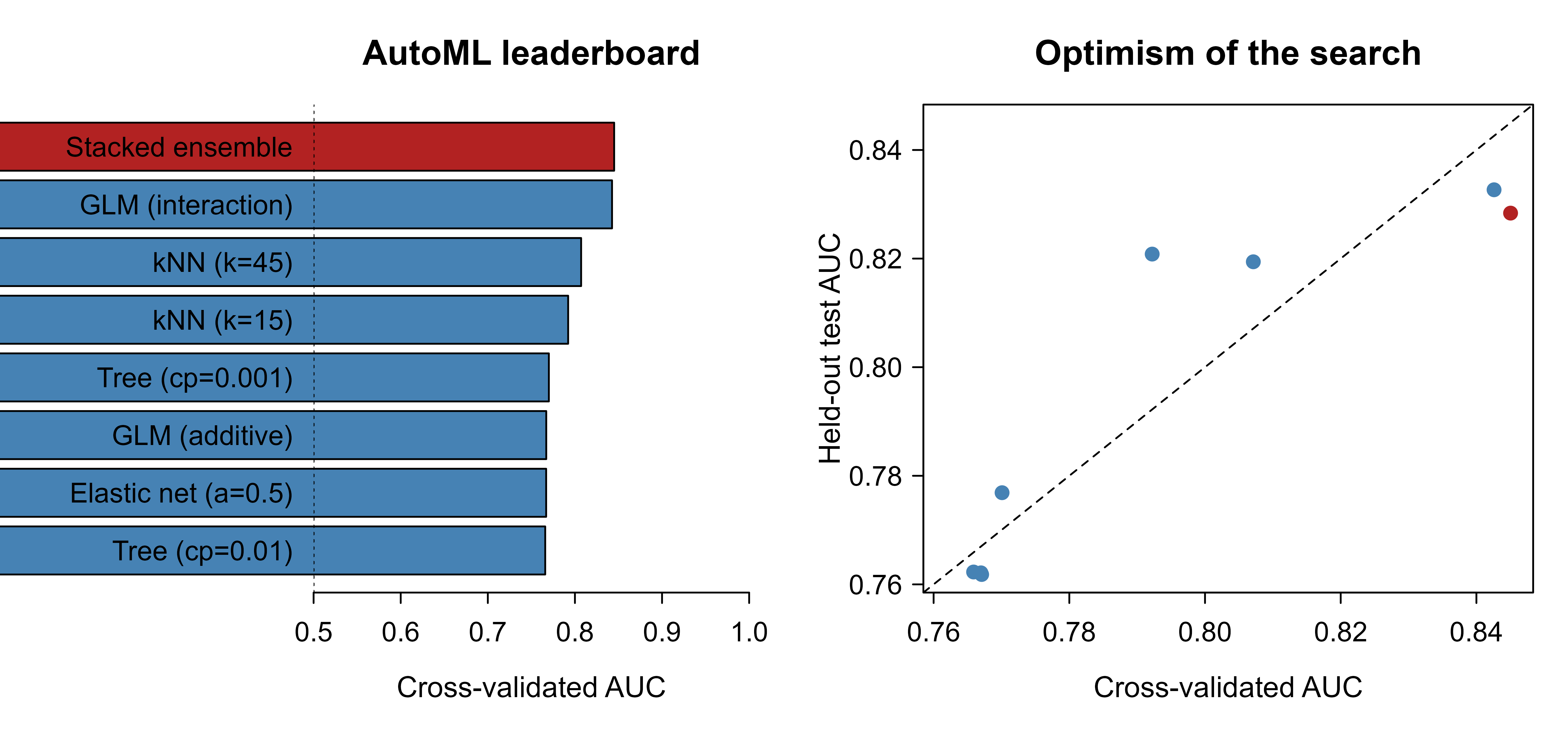

Figure 98.1: Left: the AutoML leaderboard, pipelines ranked by out-of-fold (cross-validated) AUC, with the stacked ensemble highlighted. Right: cross-validated AUC against held-out test AUC for each pipeline; points below the dashed diagonal scored better in cross-validation than on truly unseen data, the gap being the optimism of the search.

The lesson the demonstration teaches is the one the formalism predicts. The CASH search finds a strong pipeline, the stacked ensemble is hard to beat, and the cross-validation score that picked the winner is mildly optimistic about its true performance. Scale the search space from seven pipelines to seven thousand and the optimism column grows, which is exactly why a held-out test set the search never touches is not optional.

98.7 Practical guidance and pitfalls

AutoML is a force multiplier when used with discipline and a trap when used as an oracle. The recurring failure modes are predictable.

• Overfitting the validation procedure. This is the central one, and the demonstration measured it. Every pipeline you evaluate is a chance to get lucky on the validation folds; reporting the maximum over many pipelines biases that maximum upward. The defense is a final test set that the search never sees, used exactly once, and treating the cross-validation score as a selection signal rather than a performance estimate. Nested cross-validation (an outer loop for honest evaluation around the inner CASH search) is the rigorous version.

• Compute cost and diminishing returns. The CASH objective is expensive: every point evaluated is a full model fit with cross-validation. Doubling the budget rarely doubles the gain. Set a wall-clock or model-count budget up front, log the best-so-far against time, and stop when the curve flattens. Bayesian optimization and meta-learning help most when the budget is tight; with a generous budget, random search closes much of the gap.

• Data leakage through preprocessing. If you impute, scale, or select features using the whole dataset before the search, information from the validation folds leaks into training and every score is optimistic. Preprocessing must live inside the cross-validation loop, fit on the training portion of each fold only. This is why mature systems treat preprocessing as part of the searched pipeline rather than a fixed step done in advance, a point the Feature Engineering chapter makes in its own right.

• The wrong objective. AutoML minimizes the metric you give it. If you optimize accuracy on an imbalanced problem, you may get a model that ignores the minority class (the class imbalance chapter, Chapter 80, treats this in depth); if you optimize a metric that does not match the business cost, you get a model optimized for the wrong thing. Choose the metric deliberately, and consider class weights or a cost-sensitive loss when the costs are asymmetric.

• Serving cost versus accuracy. AutoML’s leader is often a large stacked ensemble that requires every base model at scoring time. The best single model is frequently within a small margin and far cheaper to serve. Compare accuracy against latency and portability, not accuracy alone.

• Reproducibility and seeds. A search with randomized trials or parallel training is only reproducible when seeds are fixed and the environment is pinned. Record the search space, the budget, the seed, and the package versions, or you cannot rerun the result.

When to use this

Reach for AutoML to get a strong baseline quickly, to search more broadly than you would by hand, or to free expert time for the parts of the problem (framing, features, evaluation) that genuinely need judgment. Do not reach for it expecting it to choose the right objective, fix leaky features, or substitute for an honest held-out evaluation. It automates the search, not the thinking around it.

98.8 Further reading

• Thornton, Hutter, Hoos, and Leyton-Brown (2013), “Auto-WEKA: Combined Selection and Hyperparameter Optimization of Classification Algorithms,” for the CASH formulation used throughout this chapter.
• Feurer, Klein, Eggensperger, Springenberg, Blum, and Hutter (2015), “Efficient and Robust Automated Machine Learning,” for auto-sklearn, meta-learning warm-starts, and ensemble selection.
• Hutter, Hoos, and Leyton-Brown (2011), “Sequential Model-Based Optimization for General Algorithm Configuration,” for the SMAC random-forest surrogate that searches the CASH space.
• Bergstra and Bengio (2012), “Random Search for Hyper-Parameter Optimization,” for why random search is the right baseline.
• Bergstra, Bardenet, Bengio, and Kegl (2011), “Algorithms for Hyper-Parameter Optimization,” for tree-structured Parzen estimators and the Bayesian-optimization view.
• Caruana, Niculescu-Mizil, Crew, and Ksikes (2004), “Ensemble Selection from Libraries of Models,” for the post-hoc ensembling that turns a leaderboard into a final model.
• Liu, Simonyan, and Yang (2019), “DARTS: Differentiable Architecture Search,” and Elsken, Metzen, and Hutter (2019), “Neural Architecture Search: A Survey,” for the NAS material.
• LeDell and Poirier (2020), “H2O AutoML: Scalable Automatic Machine Learning,” for the design of h2o.automl.
• Hutter, Kotthoff, and Vanschoren, editors (2019), Automated Machine Learning: Methods, Systems, Challenges, for a book-length treatment of the whole field.

:::{#quarto-navigation-envelope .hidden}
[Advanced Data Analysis]{.hidden .quarto-markdown-envelope-contents render-id="cXVhcnRvLWludC1zaWRlYmFyLXRpdGxl"}
[Advanced Data Analysis]{.hidden .quarto-markdown-envelope-contents render-id="cXVhcnRvLWludC1uYXZiYXItdGl0bGU="}
[<span class='chapter-number'>99</span>  <span class='chapter-title'>Databases and SQL from R</span>]{.hidden .quarto-markdown-envelope-contents render-id="cXVhcnRvLWludC1uZXh0"}
[<span class='chapter-number'>97</span>  <span class='chapter-title'>Scalable Machine Learning with h2o</span>]{.hidden .quarto-markdown-envelope-contents render-id="cXVhcnRvLWludC1wcmV2"}
[Preface]{.hidden .quarto-markdown-envelope-contents render-id="cXVhcnRvLWludC1zaWRlYmFyOi9pbmRleC5odG1sUHJlZmFjZQ=="}
[Machine Learning]{.hidden .quarto-markdown-envelope-contents render-id="cXVhcnRvLWludC1zaWRlYmFyOnF1YXJ0by1zaWRlYmFyLXNlY3Rpb24tMQ=="}
[<span class='chapter-number'>1</span>  <span class='chapter-title'>Introduction</span>]{.hidden .quarto-markdown-envelope-contents render-id="cXVhcnRvLWludC1zaWRlYmFyOi8wMDItaW50cm8uaHRtbDxzcGFuLWNsYXNzPSdjaGFwdGVyLW51bWJlcic+MTwvc3Bhbj4tLTxzcGFuLWNsYXNzPSdjaGFwdGVyLXRpdGxlJz5JbnRyb2R1Y3Rpb248L3NwYW4+"}
[<span class='chapter-number'>2</span>  <span class='chapter-title'>Overview of Learning Paradigms</span>]{.hidden .quarto-markdown-envelope-contents render-id="cXVhcnRvLWludC1zaWRlYmFyOi8wMDMtb3ZlcnZpZXcuaHRtbDxzcGFuLWNsYXNzPSdjaGFwdGVyLW51bWJlcic+Mjwvc3Bhbj4tLTxzcGFuLWNsYXNzPSdjaGFwdGVyLXRpdGxlJz5PdmVydmlldy1vZi1MZWFybmluZy1QYXJhZGlnbXM8L3NwYW4+"}
[Supervised Learning: Local-Based Methods]{.hidden .quarto-markdown-envelope-contents render-id="cXVhcnRvLWludC1zaWRlYmFyOnF1YXJ0by1zaWRlYmFyLXNlY3Rpb24tMg=="}
[<span class='chapter-number'>3</span>  <span class='chapter-title'>Spline Regression</span>]{.hidden .quarto-markdown-envelope-contents render-id="cXVhcnRvLWludC1zaWRlYmFyOi8wMDUtc3BsaW5lLmh0bWw8c3Bhbi1jbGFzcz0nY2hhcHRlci1udW1iZXInPjM8L3NwYW4+LS08c3Bhbi1jbGFzcz0nY2hhcHRlci10aXRsZSc+U3BsaW5lLVJlZ3Jlc3Npb248L3NwYW4+"}
[<span class='chapter-number'>4</span>  <span class='chapter-title'>Kernel Smoothing</span>]{.hidden .quarto-markdown-envelope-contents render-id="cXVhcnRvLWludC1zaWRlYmFyOi8wMDYta2VybmVsLmh0bWw8c3Bhbi1jbGFzcz0nY2hhcHRlci1udW1iZXInPjQ8L3NwYW4+LS08c3Bhbi1jbGFzcz0nY2hhcHRlci10aXRsZSc+S2VybmVsLVNtb290aGluZzwvc3Bhbj4="}
[<span class='chapter-number'>5</span>  <span class='chapter-title'>Local Regression</span>]{.hidden .quarto-markdown-envelope-contents render-id="cXVhcnRvLWludC1zaWRlYmFyOi8wMDctbG9jYWwuaHRtbDxzcGFuLWNsYXNzPSdjaGFwdGVyLW51bWJlcic+NTwvc3Bhbj4tLTxzcGFuLWNsYXNzPSdjaGFwdGVyLXRpdGxlJz5Mb2NhbC1SZWdyZXNzaW9uPC9zcGFuPg=="}
[Supervised Learning: Transformation-Based Methods]{.hidden .quarto-markdown-envelope-contents render-id="cXVhcnRvLWludC1zaWRlYmFyOnF1YXJ0by1zaWRlYmFyLXNlY3Rpb24tMw=="}
[<span class='chapter-number'>6</span>  <span class='chapter-title'>Generalized Additive Models</span>]{.hidden .quarto-markdown-envelope-contents render-id="cXVhcnRvLWludC1zaWRlYmFyOi8wMDktZ2FtLmh0bWw8c3Bhbi1jbGFzcz0nY2hhcHRlci1udW1iZXInPjY8L3NwYW4+LS08c3Bhbi1jbGFzcz0nY2hhcHRlci10aXRsZSc+R2VuZXJhbGl6ZWQtQWRkaXRpdmUtTW9kZWxzPC9zcGFuPg=="}
[<span class='chapter-number'>7</span>  <span class='chapter-title'>Gaussian Process Regression</span>]{.hidden .quarto-markdown-envelope-contents render-id="cXVhcnRvLWludC1zaWRlYmFyOi8wMTAtZ2F1c3NpYW4tcHJvY2Vzcy1yZWcuaHRtbDxzcGFuLWNsYXNzPSdjaGFwdGVyLW51bWJlcic+Nzwvc3Bhbj4tLTxzcGFuLWNsYXNzPSdjaGFwdGVyLXRpdGxlJz5HYXVzc2lhbi1Qcm9jZXNzLVJlZ3Jlc3Npb248L3NwYW4+"}
[Supervised Learning: Tree-Based Methods]{.hidden .quarto-markdown-envelope-contents render-id="cXVhcnRvLWludC1zaWRlYmFyOnF1YXJ0by1zaWRlYmFyLXNlY3Rpb24tNA=="}
[<span class='chapter-number'>8</span>  <span class='chapter-title'>Classification and Regression Trees</span>]{.hidden .quarto-markdown-envelope-contents render-id="cXVhcnRvLWludC1zaWRlYmFyOi8wMTItcmVncmVzc2lvbi10cmVlcy5odG1sPHNwYW4tY2xhc3M9J2NoYXB0ZXItbnVtYmVyJz44PC9zcGFuPi0tPHNwYW4tY2xhc3M9J2NoYXB0ZXItdGl0bGUnPkNsYXNzaWZpY2F0aW9uLWFuZC1SZWdyZXNzaW9uLVRyZWVzPC9zcGFuPg=="}
[<span class='chapter-number'>9</span>  <span class='chapter-title'>Multivariate Adaptive Regression Splines</span>]{.hidden .quarto-markdown-envelope-contents render-id="cXVhcnRvLWludC1zaWRlYmFyOi8wMTMtTUFSUy5odG1sPHNwYW4tY2xhc3M9J2NoYXB0ZXItbnVtYmVyJz45PC9zcGFuPi0tPHNwYW4tY2xhc3M9J2NoYXB0ZXItdGl0bGUnPk11bHRpdmFyaWF0ZS1BZGFwdGl2ZS1SZWdyZXNzaW9uLVNwbGluZXM8L3NwYW4+"}
[<span class='chapter-number'>10</span>  <span class='chapter-title'>Bagging</span>]{.hidden .quarto-markdown-envelope-contents render-id="cXVhcnRvLWludC1zaWRlYmFyOi8wMTQtYmFnZ2luZy5odG1sPHNwYW4tY2xhc3M9J2NoYXB0ZXItbnVtYmVyJz4xMDwvc3Bhbj4tLTxzcGFuLWNsYXNzPSdjaGFwdGVyLXRpdGxlJz5CYWdnaW5nPC9zcGFuPg=="}
[<span class='chapter-number'>11</span>  <span class='chapter-title'>Boosting</span>]{.hidden .quarto-markdown-envelope-contents render-id="cXVhcnRvLWludC1zaWRlYmFyOi8wMTUtYm9vc3RpbmcuaHRtbDxzcGFuLWNsYXNzPSdjaGFwdGVyLW51bWJlcic+MTE8L3NwYW4+LS08c3Bhbi1jbGFzcz0nY2hhcHRlci10aXRsZSc+Qm9vc3Rpbmc8L3NwYW4+"}
[<span class='chapter-number'>12</span>  <span class='chapter-title'>Gradient Boosting in Practice</span>]{.hidden .quarto-markdown-envelope-contents render-id="cXVhcnRvLWludC1zaWRlYmFyOi8wMTYtZ3JhZGllbnQtYm9vc3RpbmcuaHRtbDxzcGFuLWNsYXNzPSdjaGFwdGVyLW51bWJlcic+MTI8L3NwYW4+LS08c3Bhbi1jbGFzcz0nY2hhcHRlci10aXRsZSc+R3JhZGllbnQtQm9vc3RpbmctaW4tUHJhY3RpY2U8L3NwYW4+"}
[<span class='chapter-number'>13</span>  <span class='chapter-title'>Random Forests</span>]{.hidden .quarto-markdown-envelope-contents render-id="cXVhcnRvLWludC1zaWRlYmFyOi8wMTctcmFuZG9tLWZvcmVzdC5odG1sPHNwYW4tY2xhc3M9J2NoYXB0ZXItbnVtYmVyJz4xMzwvc3Bhbj4tLTxzcGFuLWNsYXNzPSdjaGFwdGVyLXRpdGxlJz5SYW5kb20tRm9yZXN0czwvc3Bhbj4="}
[<span class='chapter-number'>14</span>  <span class='chapter-title'>Bayesian Additive Regression Trees</span>]{.hidden .quarto-markdown-envelope-contents render-id="cXVhcnRvLWludC1zaWRlYmFyOi8wMTgtQkFSVC5odG1sPHNwYW4tY2xhc3M9J2NoYXB0ZXItbnVtYmVyJz4xNDwvc3Bhbj4tLTxzcGFuLWNsYXNzPSdjaGFwdGVyLXRpdGxlJz5CYXllc2lhbi1BZGRpdGl2ZS1SZWdyZXNzaW9uLVRyZWVzPC9zcGFuPg=="}
[Supervised Learning: Neural Networks]{.hidden .quarto-markdown-envelope-contents render-id="cXVhcnRvLWludC1zaWRlYmFyOnF1YXJ0by1zaWRlYmFyLXNlY3Rpb24tNQ=="}
[<span class='chapter-number'>15</span>  <span class='chapter-title'>Neural Networks</span>]{.hidden .quarto-markdown-envelope-contents render-id="cXVhcnRvLWludC1zaWRlYmFyOi8wMjAtbmV1cmFsLW5ldHdvcmtzLmh0bWw8c3Bhbi1jbGFzcz0nY2hhcHRlci1udW1iZXInPjE1PC9zcGFuPi0tPHNwYW4tY2xhc3M9J2NoYXB0ZXItdGl0bGUnPk5ldXJhbC1OZXR3b3Jrczwvc3Bhbj4="}
[<span class='chapter-number'>16</span>  <span class='chapter-title'>Artificial Intelligence</span>]{.hidden .quarto-markdown-envelope-contents render-id="cXVhcnRvLWludC1zaWRlYmFyOi8wMjEtQUkuaHRtbDxzcGFuLWNsYXNzPSdjaGFwdGVyLW51bWJlcic+MTY8L3NwYW4+LS08c3Bhbi1jbGFzcz0nY2hhcHRlci10aXRsZSc+QXJ0aWZpY2lhbC1JbnRlbGxpZ2VuY2U8L3NwYW4+"}
[Supervised Learning: Other Methods]{.hidden .quarto-markdown-envelope-contents render-id="cXVhcnRvLWludC1zaWRlYmFyOnF1YXJ0by1zaWRlYmFyLXNlY3Rpb24tNg=="}
[<span class='chapter-number'>17</span>  <span class='chapter-title'>k-Nearest Neighbors</span>]{.hidden .quarto-markdown-envelope-contents render-id="cXVhcnRvLWludC1zaWRlYmFyOi8wMjMta25uLmh0bWw8c3Bhbi1jbGFzcz0nY2hhcHRlci1udW1iZXInPjE3PC9zcGFuPi0tPHNwYW4tY2xhc3M9J2NoYXB0ZXItdGl0bGUnPmstTmVhcmVzdC1OZWlnaGJvcnM8L3NwYW4+"}
[<span class='chapter-number'>18</span>  <span class='chapter-title'>Naive Bayes</span>]{.hidden .quarto-markdown-envelope-contents render-id="cXVhcnRvLWludC1zaWRlYmFyOi8wMjQtbmFpdmUtYmF5ZXMuaHRtbDxzcGFuLWNsYXNzPSdjaGFwdGVyLW51bWJlcic+MTg8L3NwYW4+LS08c3Bhbi1jbGFzcz0nY2hhcHRlci10aXRsZSc+TmFpdmUtQmF5ZXM8L3NwYW4+"}
[<span class='chapter-number'>19</span>  <span class='chapter-title'>Support Vector</span>]{.hidden .quarto-markdown-envelope-contents render-id="cXVhcnRvLWludC1zaWRlYmFyOi8wMjUtc3ZtLmh0bWw8c3Bhbi1jbGFzcz0nY2hhcHRlci1udW1iZXInPjE5PC9zcGFuPi0tPHNwYW4tY2xhc3M9J2NoYXB0ZXItdGl0bGUnPlN1cHBvcnQtVmVjdG9yPC9zcGFuPg=="}
[<span class='chapter-number'>20</span>  <span class='chapter-title'>Discriminant Analysis</span>]{.hidden .quarto-markdown-envelope-contents render-id="cXVhcnRvLWludC1zaWRlYmFyOi8wMjYtZGlzY3JpbWluYW50LWFuYWx5c2lzLmh0bWw8c3Bhbi1jbGFzcz0nY2hhcHRlci1udW1iZXInPjIwPC9zcGFuPi0tPHNwYW4tY2xhc3M9J2NoYXB0ZXItdGl0bGUnPkRpc2NyaW1pbmFudC1BbmFseXNpczwvc3Bhbj4="}
[<span class='chapter-number'>21</span>  <span class='chapter-title'>Quantile Regression</span>]{.hidden .quarto-markdown-envelope-contents render-id="cXVhcnRvLWludC1zaWRlYmFyOi8wMjctcXVhbnRpbGUtcmVnLmh0bWw8c3Bhbi1jbGFzcz0nY2hhcHRlci1udW1iZXInPjIxPC9zcGFuPi0tPHNwYW4tY2xhc3M9J2NoYXB0ZXItdGl0bGUnPlF1YW50aWxlLVJlZ3Jlc3Npb248L3NwYW4+"}
[Unsupervised Learning: Clustering]{.hidden .quarto-markdown-envelope-contents render-id="cXVhcnRvLWludC1zaWRlYmFyOnF1YXJ0by1zaWRlYmFyLXNlY3Rpb24tNw=="}
[<span class='chapter-number'>22</span>  <span class='chapter-title'>Introduction</span>]{.hidden .quarto-markdown-envelope-contents render-id="cXVhcnRvLWludC1zaWRlYmFyOi8wMjktaW50cm8tdW5zdXBlcnZpc2VkLmh0bWw8c3Bhbi1jbGFzcz0nY2hhcHRlci1udW1iZXInPjIyPC9zcGFuPi0tPHNwYW4tY2xhc3M9J2NoYXB0ZXItdGl0bGUnPkludHJvZHVjdGlvbjwvc3Bhbj4="}
[<span class='chapter-number'>23</span>  <span class='chapter-title'>Cluster Analysis</span>]{.hidden .quarto-markdown-envelope-contents render-id="cXVhcnRvLWludC1zaWRlYmFyOi8wMzAtY2x1c3Rlci5odG1sPHNwYW4tY2xhc3M9J2NoYXB0ZXItbnVtYmVyJz4yMzwvc3Bhbj4tLTxzcGFuLWNsYXNzPSdjaGFwdGVyLXRpdGxlJz5DbHVzdGVyLUFuYWx5c2lzPC9zcGFuPg=="}
[<span class='chapter-number'>24</span>  <span class='chapter-title'>Gaussian Mixture Models and the EM Algorithm</span>]{.hidden .quarto-markdown-envelope-contents render-id="cXVhcnRvLWludC1zaWRlYmFyOi8wMzBhLWdtbS1lbS5odG1sPHNwYW4tY2xhc3M9J2NoYXB0ZXItbnVtYmVyJz4yNDwvc3Bhbj4tLTxzcGFuLWNsYXNzPSdjaGFwdGVyLXRpdGxlJz5HYXVzc2lhbi1NaXh0dXJlLU1vZGVscy1hbmQtdGhlLUVNLUFsZ29yaXRobTwvc3Bhbj4="}
[<span class='chapter-number'>25</span>  <span class='chapter-title'>Spectral Clustering</span>]{.hidden .quarto-markdown-envelope-contents render-id="cXVhcnRvLWludC1zaWRlYmFyOi8wMzBiLXNwZWN0cmFsLWNsdXN0ZXJpbmcuaHRtbDxzcGFuLWNsYXNzPSdjaGFwdGVyLW51bWJlcic+MjU8L3NwYW4+LS08c3Bhbi1jbGFzcz0nY2hhcHRlci10aXRsZSc+U3BlY3RyYWwtQ2x1c3RlcmluZzwvc3Bhbj4="}
[<span class='chapter-number'>26</span>  <span class='chapter-title'>Self-Organizing Maps</span>]{.hidden .quarto-markdown-envelope-contents render-id="cXVhcnRvLWludC1zaWRlYmFyOi8wMzBjLXNlbGYtb3JnYW5pemluZy1tYXBzLmh0bWw8c3Bhbi1jbGFzcz0nY2hhcHRlci1udW1iZXInPjI2PC9zcGFuPi0tPHNwYW4tY2xhc3M9J2NoYXB0ZXItdGl0bGUnPlNlbGYtT3JnYW5pemluZy1NYXBzPC9zcGFuPg=="}
[Unsupervised Learning: Dimension Reduction and Representation]{.hidden .quarto-markdown-envelope-contents render-id="cXVhcnRvLWludC1zaWRlYmFyOnF1YXJ0by1zaWRlYmFyLXNlY3Rpb24tOA=="}
[<span class='chapter-number'>27</span>  <span class='chapter-title'>Dimension Reduction</span>]{.hidden .quarto-markdown-envelope-contents render-id="cXVhcnRvLWludC1zaWRlYmFyOi8wMzEtZGltZW5zaW9uLXJlZHVjdGlvbi5odG1sPHNwYW4tY2xhc3M9J2NoYXB0ZXItbnVtYmVyJz4yNzwvc3Bhbj4tLTxzcGFuLWNsYXNzPSdjaGFwdGVyLXRpdGxlJz5EaW1lbnNpb24tUmVkdWN0aW9uPC9zcGFuPg=="}
[<span class='chapter-number'>28</span>  <span class='chapter-title'>Independent Component Analysis</span>]{.hidden .quarto-markdown-envelope-contents render-id="cXVhcnRvLWludC1zaWRlYmFyOi8wMzFhLWljYS5odG1sPHNwYW4tY2xhc3M9J2NoYXB0ZXItbnVtYmVyJz4yODwvc3Bhbj4tLTxzcGFuLWNsYXNzPSdjaGFwdGVyLXRpdGxlJz5JbmRlcGVuZGVudC1Db21wb25lbnQtQW5hbHlzaXM8L3NwYW4+"}
[<span class='chapter-number'>29</span>  <span class='chapter-title'>Non-negative Matrix Factorization</span>]{.hidden .quarto-markdown-envelope-contents render-id="cXVhcnRvLWludC1zaWRlYmFyOi8wMzFiLW5tZi5odG1sPHNwYW4tY2xhc3M9J2NoYXB0ZXItbnVtYmVyJz4yOTwvc3Bhbj4tLTxzcGFuLWNsYXNzPSdjaGFwdGVyLXRpdGxlJz5Ob24tbmVnYXRpdmUtTWF0cml4LUZhY3Rvcml6YXRpb248L3NwYW4+"}
[<span class='chapter-number'>30</span>  <span class='chapter-title'>Factor Analysis</span>]{.hidden .quarto-markdown-envelope-contents render-id="cXVhcnRvLWludC1zaWRlYmFyOi8wMzFjLWZhY3Rvci1hbmFseXNpcy5odG1sPHNwYW4tY2xhc3M9J2NoYXB0ZXItbnVtYmVyJz4zMDwvc3Bhbj4tLTxzcGFuLWNsYXNzPSdjaGFwdGVyLXRpdGxlJz5GYWN0b3ItQW5hbHlzaXM8L3NwYW4+"}
[<span class='chapter-number'>31</span>  <span class='chapter-title'>Multidimensional Scaling and Nonlinear Dimension Reduction</span>]{.hidden .quarto-markdown-envelope-contents render-id="cXVhcnRvLWludC1zaWRlYmFyOi8wMzItc2NhbGluZy5odG1sPHNwYW4tY2xhc3M9J2NoYXB0ZXItbnVtYmVyJz4zMTwvc3Bhbj4tLTxzcGFuLWNsYXNzPSdjaGFwdGVyLXRpdGxlJz5NdWx0aWRpbWVuc2lvbmFsLVNjYWxpbmctYW5kLU5vbmxpbmVhci1EaW1lbnNpb24tUmVkdWN0aW9uPC9zcGFuPg=="}
[Unsupervised Learning: Density, Patterns, and Interpretability]{.hidden .quarto-markdown-envelope-contents render-id="cXVhcnRvLWludC1zaWRlYmFyOnF1YXJ0by1zaWRlYmFyLXNlY3Rpb24tOQ=="}
[<span class='chapter-number'>32</span>  <span class='chapter-title'>Density Estimation</span>]{.hidden .quarto-markdown-envelope-contents render-id="cXVhcnRvLWludC1zaWRlYmFyOi8wMzQtZGVuc2l0eS1lc3RpbWF0aW9uLmh0bWw8c3Bhbi1jbGFzcz0nY2hhcHRlci1udW1iZXInPjMyPC9zcGFuPi0tPHNwYW4tY2xhc3M9J2NoYXB0ZXItdGl0bGUnPkRlbnNpdHktRXN0aW1hdGlvbjwvc3Bhbj4="}
[<span class='chapter-number'>33</span>  <span class='chapter-title'>Association Rule Mining</span>]{.hidden .quarto-markdown-envelope-contents render-id="cXVhcnRvLWludC1zaWRlYmFyOi8wMzNhLWFzc29jaWF0aW9uLXJ1bGVzLmh0bWw8c3Bhbi1jbGFzcz0nY2hhcHRlci1udW1iZXInPjMzPC9zcGFuPi0tPHNwYW4tY2xhc3M9J2NoYXB0ZXItdGl0bGUnPkFzc29jaWF0aW9uLVJ1bGUtTWluaW5nPC9zcGFuPg=="}
[<span class='chapter-number'>34</span>  <span class='chapter-title'>Topic Models and Latent Dirichlet Allocation</span>]{.hidden .quarto-markdown-envelope-contents render-id="cXVhcnRvLWludC1zaWRlYmFyOi8wMzNiLXRvcGljLW1vZGVscy5odG1sPHNwYW4tY2xhc3M9J2NoYXB0ZXItbnVtYmVyJz4zNDwvc3Bhbj4tLTxzcGFuLWNsYXNzPSdjaGFwdGVyLXRpdGxlJz5Ub3BpYy1Nb2RlbHMtYW5kLUxhdGVudC1EaXJpY2hsZXQtQWxsb2NhdGlvbjwvc3Bhbj4="}
[<span class='chapter-number'>35</span>  <span class='chapter-title'>Interpretable Machine Learning</span>]{.hidden .quarto-markdown-envelope-contents render-id="cXVhcnRvLWludC1zaWRlYmFyOi8wMzMtaW50ZXJwcmV0YWJsZS1tYWNoaW5lLWxlYXJuaW5nLmh0bWw8c3Bhbi1jbGFzcz0nY2hhcHRlci1udW1iZXInPjM1PC9zcGFuPi0tPHNwYW4tY2xhc3M9J2NoYXB0ZXItdGl0bGUnPkludGVycHJldGFibGUtTWFjaGluZS1MZWFybmluZzwvc3Bhbj4="}
[Deep Learning]{.hidden .quarto-markdown-envelope-contents render-id="cXVhcnRvLWludC1zaWRlYmFyOnF1YXJ0by1zaWRlYmFyLXNlY3Rpb24tMTA="}
[<span class='chapter-number'>36</span>  <span class='chapter-title'>Convolutional Neural Networks</span>]{.hidden .quarto-markdown-envelope-contents render-id="cXVhcnRvLWludC1zaWRlYmFyOi8wMzVhLWNubi5odG1sPHNwYW4tY2xhc3M9J2NoYXB0ZXItbnVtYmVyJz4zNjwvc3Bhbj4tLTxzcGFuLWNsYXNzPSdjaGFwdGVyLXRpdGxlJz5Db252b2x1dGlvbmFsLU5ldXJhbC1OZXR3b3Jrczwvc3Bhbj4="}
[<span class='chapter-number'>37</span>  <span class='chapter-title'>Recurrent Neural Networks: LSTMs and GRUs</span>]{.hidden .quarto-markdown-envelope-contents render-id="cXVhcnRvLWludC1zaWRlYmFyOi8wMzViLXJubi5odG1sPHNwYW4tY2xhc3M9J2NoYXB0ZXItbnVtYmVyJz4zNzwvc3Bhbj4tLTxzcGFuLWNsYXNzPSdjaGFwdGVyLXRpdGxlJz5SZWN1cnJlbnQtTmV1cmFsLU5ldHdvcmtzOi1MU1RNcy1hbmQtR1JVczwvc3Bhbj4="}
[<span class='chapter-number'>38</span>  <span class='chapter-title'>Attention and Transformers</span>]{.hidden .quarto-markdown-envelope-contents render-id="cXVhcnRvLWludC1zaWRlYmFyOi8wMzYtdHJhbnNmb3JtZXJzLmh0bWw8c3Bhbi1jbGFzcz0nY2hhcHRlci1udW1iZXInPjM4PC9zcGFuPi0tPHNwYW4tY2xhc3M9J2NoYXB0ZXItdGl0bGUnPkF0dGVudGlvbi1hbmQtVHJhbnNmb3JtZXJzPC9zcGFuPg=="}
[<span class='chapter-number'>39</span>  <span class='chapter-title'>BERT</span>]{.hidden .quarto-markdown-envelope-contents render-id="cXVhcnRvLWludC1zaWRlYmFyOi8wMzctQkVSVC5odG1sPHNwYW4tY2xhc3M9J2NoYXB0ZXItbnVtYmVyJz4zOTwvc3Bhbj4tLTxzcGFuLWNsYXNzPSdjaGFwdGVyLXRpdGxlJz5CRVJUPC9zcGFuPg=="}
[<span class='chapter-number'>40</span>  <span class='chapter-title'>Large Language Models and Foundation Models</span>]{.hidden .quarto-markdown-envelope-contents render-id="cXVhcnRvLWludC1zaWRlYmFyOi8wMzgtbGxtcy5odG1sPHNwYW4tY2xhc3M9J2NoYXB0ZXItbnVtYmVyJz40MDwvc3Bhbj4tLTxzcGFuLWNsYXNzPSdjaGFwdGVyLXRpdGxlJz5MYXJnZS1MYW5ndWFnZS1Nb2RlbHMtYW5kLUZvdW5kYXRpb24tTW9kZWxzPC9zcGFuPg=="}
[<span class='chapter-number'>41</span>  <span class='chapter-title'>Autoencoders and Representation Learning</span>]{.hidden .quarto-markdown-envelope-contents render-id="cXVhcnRvLWludC1zaWRlYmFyOi8wMzktYXV0b2VuY29kZXJzLmh0bWw8c3Bhbi1jbGFzcz0nY2hhcHRlci1udW1iZXInPjQxPC9zcGFuPi0tPHNwYW4tY2xhc3M9J2NoYXB0ZXItdGl0bGUnPkF1dG9lbmNvZGVycy1hbmQtUmVwcmVzZW50YXRpb24tTGVhcm5pbmc8L3NwYW4+"}
[<span class='chapter-number'>42</span>  <span class='chapter-title'>Generative Models</span>]{.hidden .quarto-markdown-envelope-contents render-id="cXVhcnRvLWludC1zaWRlYmFyOi8wNDAtZ2VuZXJhdGl2ZS1tb2RlbHMuaHRtbDxzcGFuLWNsYXNzPSdjaGFwdGVyLW51bWJlcic+NDI8L3NwYW4+LS08c3Bhbi1jbGFzcz0nY2hhcHRlci10aXRsZSc+R2VuZXJhdGl2ZS1Nb2RlbHM8L3NwYW4+"}
[<span class='chapter-number'>43</span>  <span class='chapter-title'>Diffusion Models</span>]{.hidden .quarto-markdown-envelope-contents render-id="cXVhcnRvLWludC1zaWRlYmFyOi8wNDBhLWRpZmZ1c2lvbi5odG1sPHNwYW4tY2xhc3M9J2NoYXB0ZXItbnVtYmVyJz40Mzwvc3Bhbj4tLTxzcGFuLWNsYXNzPSdjaGFwdGVyLXRpdGxlJz5EaWZmdXNpb24tTW9kZWxzPC9zcGFuPg=="}
[<span class='chapter-number'>44</span>  <span class='chapter-title'>Graph Neural Networks</span>]{.hidden .quarto-markdown-envelope-contents render-id="cXVhcnRvLWludC1zaWRlYmFyOi8wNDEtZ3JhcGgtbmV1cmFsLW5ldHdvcmtzLmh0bWw8c3Bhbi1jbGFzcz0nY2hhcHRlci1udW1iZXInPjQ0PC9zcGFuPi0tPHNwYW4tY2xhc3M9J2NoYXB0ZXItdGl0bGUnPkdyYXBoLU5ldXJhbC1OZXR3b3Jrczwvc3Bhbj4="}
[<span class='chapter-number'>45</span>  <span class='chapter-title'>Mixture of Experts and Conditional Computation</span>]{.hidden .quarto-markdown-envelope-contents render-id="cXVhcnRvLWludC1zaWRlYmFyOi8wNDItbWl4dHVyZS1vZi1leHBlcnRzLmh0bWw8c3Bhbi1jbGFzcz0nY2hhcHRlci1udW1iZXInPjQ1PC9zcGFuPi0tPHNwYW4tY2xhc3M9J2NoYXB0ZXItdGl0bGUnPk1peHR1cmUtb2YtRXhwZXJ0cy1hbmQtQ29uZGl0aW9uYWwtQ29tcHV0YXRpb248L3NwYW4+"}
[<span class='chapter-number'>46</span>  <span class='chapter-title'>Bayesian Deep Learning and Uncertainty Quantification</span>]{.hidden .quarto-markdown-envelope-contents render-id="cXVhcnRvLWludC1zaWRlYmFyOi8wNDMtYmF5ZXNpYW4tZGVlcC1sZWFybmluZy5odG1sPHNwYW4tY2xhc3M9J2NoYXB0ZXItbnVtYmVyJz40Njwvc3Bhbj4tLTxzcGFuLWNsYXNzPSdjaGFwdGVyLXRpdGxlJz5CYXllc2lhbi1EZWVwLUxlYXJuaW5nLWFuZC1VbmNlcnRhaW50eS1RdWFudGlmaWNhdGlvbjwvc3Bhbj4="}
[<span class='chapter-number'>47</span>  <span class='chapter-title'>Double Descent</span>]{.hidden .quarto-markdown-envelope-contents render-id="cXVhcnRvLWludC1zaWRlYmFyOi8wNDNiLWRvdWJsZS1kZXNjZW50Lmh0bWw8c3Bhbi1jbGFzcz0nY2hhcHRlci1udW1iZXInPjQ3PC9zcGFuPi0tPHNwYW4tY2xhc3M9J2NoYXB0ZXItdGl0bGUnPkRvdWJsZS1EZXNjZW50PC9zcGFuPg=="}
[Learning Paradigms]{.hidden .quarto-markdown-envelope-contents render-id="cXVhcnRvLWludC1zaWRlYmFyOnF1YXJ0by1zaWRlYmFyLXNlY3Rpb24tMTE="}
[<span class='chapter-number'>48</span>  <span class='chapter-title'>Semi-Supervised Learning</span>]{.hidden .quarto-markdown-envelope-contents render-id="cXVhcnRvLWludC1zaWRlYmFyOi8wNDUtc2VtaS1zdXBlcnZpc2VkLWxlYXJuaW5nLmh0bWw8c3Bhbi1jbGFzcz0nY2hhcHRlci1udW1iZXInPjQ4PC9zcGFuPi0tPHNwYW4tY2xhc3M9J2NoYXB0ZXItdGl0bGUnPlNlbWktU3VwZXJ2aXNlZC1MZWFybmluZzwvc3Bhbj4="}
[<span class='chapter-number'>49</span>  <span class='chapter-title'>Self-Supervised and Contrastive Learning</span>]{.hidden .quarto-markdown-envelope-contents render-id="cXVhcnRvLWludC1zaWRlYmFyOi8wNDYtc2VsZi1zdXBlcnZpc2VkLWxlYXJuaW5nLmh0bWw8c3Bhbi1jbGFzcz0nY2hhcHRlci1udW1iZXInPjQ5PC9zcGFuPi0tPHNwYW4tY2xhc3M9J2NoYXB0ZXItdGl0bGUnPlNlbGYtU3VwZXJ2aXNlZC1hbmQtQ29udHJhc3RpdmUtTGVhcm5pbmc8L3NwYW4+"}
[<span class='chapter-number'>50</span>  <span class='chapter-title'>Active Learning</span>]{.hidden .quarto-markdown-envelope-contents render-id="cXVhcnRvLWludC1zaWRlYmFyOi8wNDctYWN0aXZlLWxlYXJuaW5nLmh0bWw8c3Bhbi1jbGFzcz0nY2hhcHRlci1udW1iZXInPjUwPC9zcGFuPi0tPHNwYW4tY2xhc3M9J2NoYXB0ZXItdGl0bGUnPkFjdGl2ZS1MZWFybmluZzwvc3Bhbj4="}
[<span class='chapter-number'>51</span>  <span class='chapter-title'>Weakly-Supervised and Positive-Unlabeled Learning</span>]{.hidden .quarto-markdown-envelope-contents render-id="cXVhcnRvLWludC1zaWRlYmFyOi8wNDgtd2Vha2x5LXN1cGVydmlzZWQtcHUuaHRtbDxzcGFuLWNsYXNzPSdjaGFwdGVyLW51bWJlcic+NTE8L3NwYW4+LS08c3Bhbi1jbGFzcz0nY2hhcHRlci10aXRsZSc+V2Vha2x5LVN1cGVydmlzZWQtYW5kLVBvc2l0aXZlLVVubGFiZWxlZC1MZWFybmluZzwvc3Bhbj4="}
[<span class='chapter-number'>52</span>  <span class='chapter-title'>Few-Shot and Zero-Shot Learning</span>]{.hidden .quarto-markdown-envelope-contents render-id="cXVhcnRvLWludC1zaWRlYmFyOi8wNDktZmV3LXNob3QtemVyby1zaG90Lmh0bWw8c3Bhbi1jbGFzcz0nY2hhcHRlci1udW1iZXInPjUyPC9zcGFuPi0tPHNwYW4tY2xhc3M9J2NoYXB0ZXItdGl0bGUnPkZldy1TaG90LWFuZC1aZXJvLVNob3QtTGVhcm5pbmc8L3NwYW4+"}
[<span class='chapter-number'>53</span>  <span class='chapter-title'>Meta-Learning and Few-Shot Learning</span>]{.hidden .quarto-markdown-envelope-contents render-id="cXVhcnRvLWludC1zaWRlYmFyOi8wNTAtbWV0YS1sZWFybmluZy5odG1sPHNwYW4tY2xhc3M9J2NoYXB0ZXItbnVtYmVyJz41Mzwvc3Bhbj4tLTxzcGFuLWNsYXNzPSdjaGFwdGVyLXRpdGxlJz5NZXRhLUxlYXJuaW5nLWFuZC1GZXctU2hvdC1MZWFybmluZzwvc3Bhbj4="}
[<span class='chapter-number'>54</span>  <span class='chapter-title'>Transfer and Multi-Task Learning</span>]{.hidden .quarto-markdown-envelope-contents render-id="cXVhcnRvLWludC1zaWRlYmFyOi8wNTEtdHJhbnNmZXItbXVsdGl0YXNrLWxlYXJuaW5nLmh0bWw8c3Bhbi1jbGFzcz0nY2hhcHRlci1udW1iZXInPjU0PC9zcGFuPi0tPHNwYW4tY2xhc3M9J2NoYXB0ZXItdGl0bGUnPlRyYW5zZmVyLWFuZC1NdWx0aS1UYXNrLUxlYXJuaW5nPC9zcGFuPg=="}
[<span class='chapter-number'>55</span>  <span class='chapter-title'>Online and Streaming Learning</span>]{.hidden .quarto-markdown-envelope-contents render-id="cXVhcnRvLWludC1zaWRlYmFyOi8wNTItb25saW5lLWxlYXJuaW5nLmh0bWw8c3Bhbi1jbGFzcz0nY2hhcHRlci1udW1iZXInPjU1PC9zcGFuPi0tPHNwYW4tY2xhc3M9J2NoYXB0ZXItdGl0bGUnPk9ubGluZS1hbmQtU3RyZWFtaW5nLUxlYXJuaW5nPC9zcGFuPg=="}
[<span class='chapter-number'>56</span>  <span class='chapter-title'>Federated Learning</span>]{.hidden .quarto-markdown-envelope-contents render-id="cXVhcnRvLWludC1zaWRlYmFyOi8wNTMtZmVkZXJhdGVkLWxlYXJuaW5nLmh0bWw8c3Bhbi1jbGFzcz0nY2hhcHRlci1udW1iZXInPjU2PC9zcGFuPi0tPHNwYW4tY2xhc3M9J2NoYXB0ZXItdGl0bGUnPkZlZGVyYXRlZC1MZWFybmluZzwvc3Bhbj4="}
[<span class='chapter-number'>57</span>  <span class='chapter-title'>Ensemble Learning</span>]{.hidden .quarto-markdown-envelope-contents render-id="cXVhcnRvLWludC1zaWRlYmFyOi8wNTQtZW5zZW1ibGUtbGVhcm5pbmcuaHRtbDxzcGFuLWNsYXNzPSdjaGFwdGVyLW51bWJlcic+NTc8L3NwYW4+LS08c3Bhbi1jbGFzcz0nY2hhcHRlci10aXRsZSc+RW5zZW1ibGUtTGVhcm5pbmc8L3NwYW4+"}
[<span class='chapter-number'>58</span>  <span class='chapter-title'>Continual and Lifelong Learning</span>]{.hidden .quarto-markdown-envelope-contents render-id="cXVhcnRvLWludC1zaWRlYmFyOi8wNTUtY29udGludWFsLWxlYXJuaW5nLmh0bWw8c3Bhbi1jbGFzcz0nY2hhcHRlci1udW1iZXInPjU4PC9zcGFuPi0tPHNwYW4tY2xhc3M9J2NoYXB0ZXItdGl0bGUnPkNvbnRpbnVhbC1hbmQtTGlmZWxvbmctTGVhcm5pbmc8L3NwYW4+"}
[<span class='chapter-number'>59</span>  <span class='chapter-title'>Curriculum Learning</span>]{.hidden .quarto-markdown-envelope-contents render-id="cXVhcnRvLWludC1zaWRlYmFyOi8wNTYtY3VycmljdWx1bS1sZWFybmluZy5odG1sPHNwYW4tY2xhc3M9J2NoYXB0ZXItbnVtYmVyJz41OTwvc3Bhbj4tLTxzcGFuLWNsYXNzPSdjaGFwdGVyLXRpdGxlJz5DdXJyaWN1bHVtLUxlYXJuaW5nPC9zcGFuPg=="}
[<span class='chapter-number'>60</span>  <span class='chapter-title'>Imitation Learning and Inverse Reinforcement Learning</span>]{.hidden .quarto-markdown-envelope-contents render-id="cXVhcnRvLWludC1zaWRlYmFyOi8wNTctaW1pdGF0aW9uLWludmVyc2UtcmwuaHRtbDxzcGFuLWNsYXNzPSdjaGFwdGVyLW51bWJlcic+NjA8L3NwYW4+LS08c3Bhbi1jbGFzcz0nY2hhcHRlci10aXRsZSc+SW1pdGF0aW9uLUxlYXJuaW5nLWFuZC1JbnZlcnNlLVJlaW5mb3JjZW1lbnQtTGVhcm5pbmc8L3NwYW4+"}
[<span class='chapter-number'>61</span>  <span class='chapter-title'>Transductive Learning</span>]{.hidden .quarto-markdown-envelope-contents render-id="cXVhcnRvLWludC1zaWRlYmFyOi8wNTgtdHJhbnNkdWN0aXZlLWxlYXJuaW5nLmh0bWw8c3Bhbi1jbGFzcz0nY2hhcHRlci1udW1iZXInPjYxPC9zcGFuPi0tPHNwYW4tY2xhc3M9J2NoYXB0ZXItdGl0bGUnPlRyYW5zZHVjdGl2ZS1MZWFybmluZzwvc3Bhbj4="}
[<span class='chapter-number'>62</span>  <span class='chapter-title'>Adversarial Learning</span>]{.hidden .quarto-markdown-envelope-contents render-id="cXVhcnRvLWludC1zaWRlYmFyOi8wNTktYWR2ZXJzYXJpYWwtbGVhcm5pbmcuaHRtbDxzcGFuLWNsYXNzPSdjaGFwdGVyLW51bWJlcic+NjI8L3NwYW4+LS08c3Bhbi1jbGFzcz0nY2hhcHRlci10aXRsZSc+QWR2ZXJzYXJpYWwtTGVhcm5pbmc8L3NwYW4+"}
[<span class='chapter-number'>63</span>  <span class='chapter-title'>Metric and Similarity Learning</span>]{.hidden .quarto-markdown-envelope-contents render-id="cXVhcnRvLWludC1zaWRlYmFyOi8wNjAtbWV0cmljLWxlYXJuaW5nLmh0bWw8c3Bhbi1jbGFzcz0nY2hhcHRlci1udW1iZXInPjYzPC9zcGFuPi0tPHNwYW4tY2xhc3M9J2NoYXB0ZXItdGl0bGUnPk1ldHJpYy1hbmQtU2ltaWxhcml0eS1MZWFybmluZzwvc3Bhbj4="}
[Reinforcement Learning]{.hidden .quarto-markdown-envelope-contents render-id="cXVhcnRvLWludC1zaWRlYmFyOnF1YXJ0by1zaWRlYmFyLXNlY3Rpb24tMTI="}
[<span class='chapter-number'>64</span>  <span class='chapter-title'>Foundations of Reinforcement Learning</span>]{.hidden .quarto-markdown-envelope-contents render-id="cXVhcnRvLWludC1zaWRlYmFyOi8wNjItcmwtZm91bmRhdGlvbnMuaHRtbDxzcGFuLWNsYXNzPSdjaGFwdGVyLW51bWJlcic+NjQ8L3NwYW4+LS08c3Bhbi1jbGFzcz0nY2hhcHRlci10aXRsZSc+Rm91bmRhdGlvbnMtb2YtUmVpbmZvcmNlbWVudC1MZWFybmluZzwvc3Bhbj4="}
[<span class='chapter-number'>65</span>  <span class='chapter-title'>Multi-Armed Bandits</span>]{.hidden .quarto-markdown-envelope-contents render-id="cXVhcnRvLWludC1zaWRlYmFyOi8wNjMtbXVsdGktYXJtZWQtYmFuZGl0cy5odG1sPHNwYW4tY2xhc3M9J2NoYXB0ZXItbnVtYmVyJz42NTwvc3Bhbj4tLTxzcGFuLWNsYXNzPSdjaGFwdGVyLXRpdGxlJz5NdWx0aS1Bcm1lZC1CYW5kaXRzPC9zcGFuPg=="}
[<span class='chapter-number'>66</span>  <span class='chapter-title'>Monte Carlo and Temporal-Difference Learning</span>]{.hidden .quarto-markdown-envelope-contents render-id="cXVhcnRvLWludC1zaWRlYmFyOi8wNjQtdGQtbGVhcm5pbmcuaHRtbDxzcGFuLWNsYXNzPSdjaGFwdGVyLW51bWJlcic+NjY8L3NwYW4+LS08c3Bhbi1jbGFzcz0nY2hhcHRlci10aXRsZSc+TW9udGUtQ2FybG8tYW5kLVRlbXBvcmFsLURpZmZlcmVuY2UtTGVhcm5pbmc8L3NwYW4+"}
[<span class='chapter-number'>67</span>  <span class='chapter-title'>Policy Gradient and Actor-Critic Methods</span>]{.hidden .quarto-markdown-envelope-contents render-id="cXVhcnRvLWludC1zaWRlYmFyOi8wNjUtcG9saWN5LWdyYWRpZW50Lmh0bWw8c3Bhbi1jbGFzcz0nY2hhcHRlci1udW1iZXInPjY3PC9zcGFuPi0tPHNwYW4tY2xhc3M9J2NoYXB0ZXItdGl0bGUnPlBvbGljeS1HcmFkaWVudC1hbmQtQWN0b3ItQ3JpdGljLU1ldGhvZHM8L3NwYW4+"}
[<span class='chapter-number'>68</span>  <span class='chapter-title'>Model-Based Reinforcement Learning and Planning</span>]{.hidden .quarto-markdown-envelope-contents render-id="cXVhcnRvLWludC1zaWRlYmFyOi8wNjYtbW9kZWwtYmFzZWQtcmwuaHRtbDxzcGFuLWNsYXNzPSdjaGFwdGVyLW51bWJlcic+Njg8L3NwYW4+LS08c3Bhbi1jbGFzcz0nY2hhcHRlci10aXRsZSc+TW9kZWwtQmFzZWQtUmVpbmZvcmNlbWVudC1MZWFybmluZy1hbmQtUGxhbm5pbmc8L3NwYW4+"}
[<span class='chapter-number'>69</span>  <span class='chapter-title'>Offline (Batch) Reinforcement Learning</span>]{.hidden .quarto-markdown-envelope-contents render-id="cXVhcnRvLWludC1zaWRlYmFyOi8wNjctb2ZmbGluZS1ybC5odG1sPHNwYW4tY2xhc3M9J2NoYXB0ZXItbnVtYmVyJz42OTwvc3Bhbj4tLTxzcGFuLWNsYXNzPSdjaGFwdGVyLXRpdGxlJz5PZmZsaW5lLShCYXRjaCktUmVpbmZvcmNlbWVudC1MZWFybmluZzwvc3Bhbj4="}
[<span class='chapter-number'>70</span>  <span class='chapter-title'>Multi-Agent Reinforcement Learning</span>]{.hidden .quarto-markdown-envelope-contents render-id="cXVhcnRvLWludC1zaWRlYmFyOi8wNjgtbXVsdGktYWdlbnQtcmwuaHRtbDxzcGFuLWNsYXNzPSdjaGFwdGVyLW51bWJlcic+NzA8L3NwYW4+LS08c3Bhbi1jbGFzcz0nY2hhcHRlci10aXRsZSc+TXVsdGktQWdlbnQtUmVpbmZvcmNlbWVudC1MZWFybmluZzwvc3Bhbj4="}
[<span class='chapter-number'>71</span>  <span class='chapter-title'>Deep Reinforcement Learning</span>]{.hidden .quarto-markdown-envelope-contents render-id="cXVhcnRvLWludC1zaWRlYmFyOi8wNjktZGVlcC1yZWluZm9yY2VtZW50LWxlYXJuaW5nLmh0bWw8c3Bhbi1jbGFzcz0nY2hhcHRlci1udW1iZXInPjcxPC9zcGFuPi0tPHNwYW4tY2xhc3M9J2NoYXB0ZXItdGl0bGUnPkRlZXAtUmVpbmZvcmNlbWVudC1MZWFybmluZzwvc3Bhbj4="}
[<span class='chapter-number'>72</span>  <span class='chapter-title'>Contextual Bandits</span>]{.hidden .quarto-markdown-envelope-contents render-id="cXVhcnRvLWludC1zaWRlYmFyOi8wNzAtY29udGV4dHVhbC1iYW5kaXRzLmh0bWw8c3Bhbi1jbGFzcz0nY2hhcHRlci1udW1iZXInPjcyPC9zcGFuPi0tPHNwYW4tY2xhc3M9J2NoYXB0ZXItdGl0bGUnPkNvbnRleHR1YWwtQmFuZGl0czwvc3Bhbj4="}
[Advanced and Probabilistic Methods]{.hidden .quarto-markdown-envelope-contents render-id="cXVhcnRvLWludC1zaWRlYmFyOnF1YXJ0by1zaWRlYmFyLXNlY3Rpb24tMTM="}
[<span class='chapter-number'>73</span>  <span class='chapter-title'>Probabilistic Graphical Models</span>]{.hidden .quarto-markdown-envelope-contents render-id="cXVhcnRvLWludC1zaWRlYmFyOi8wNzFhLWdyYXBoaWNhbC1tb2RlbHMuaHRtbDxzcGFuLWNsYXNzPSdjaGFwdGVyLW51bWJlcic+NzM8L3NwYW4+LS08c3Bhbi1jbGFzcz0nY2hhcHRlci10aXRsZSc+UHJvYmFiaWxpc3RpYy1HcmFwaGljYWwtTW9kZWxzPC9zcGFuPg=="}
[<span class='chapter-number'>74</span>  <span class='chapter-title'>Hidden Markov Models</span>]{.hidden .quarto-markdown-envelope-contents render-id="cXVhcnRvLWludC1zaWRlYmFyOi8wNzFiLWhtbS5odG1sPHNwYW4tY2xhc3M9J2NoYXB0ZXItbnVtYmVyJz43NDwvc3Bhbj4tLTxzcGFuLWNsYXNzPSdjaGFwdGVyLXRpdGxlJz5IaWRkZW4tTWFya292LU1vZGVsczwvc3Bhbj4="}
[<span class='chapter-number'>75</span>  <span class='chapter-title'>Probabilistic Programming with Stan and brms</span>]{.hidden .quarto-markdown-envelope-contents render-id="cXVhcnRvLWludC1zaWRlYmFyOi8wNzItcHJvYmFiaWxpc3RpYy1wcm9ncmFtbWluZy5odG1sPHNwYW4tY2xhc3M9J2NoYXB0ZXItbnVtYmVyJz43NTwvc3Bhbj4tLTxzcGFuLWNsYXNzPSdjaGFwdGVyLXRpdGxlJz5Qcm9iYWJpbGlzdGljLVByb2dyYW1taW5nLXdpdGgtU3Rhbi1hbmQtYnJtczwvc3Bhbj4="}
[<span class='chapter-number'>76</span>  <span class='chapter-title'>Causal Machine Learning and Uplift Modeling</span>]{.hidden .quarto-markdown-envelope-contents render-id="cXVhcnRvLWludC1zaWRlYmFyOi8wNzMtY2F1c2FsLW1hY2hpbmUtbGVhcm5pbmcuaHRtbDxzcGFuLWNsYXNzPSdjaGFwdGVyLW51bWJlcic+NzY8L3NwYW4+LS08c3Bhbi1jbGFzcz0nY2hhcHRlci10aXRsZSc+Q2F1c2FsLU1hY2hpbmUtTGVhcm5pbmctYW5kLVVwbGlmdC1Nb2RlbGluZzwvc3Bhbj4="}
[<span class='chapter-number'>77</span>  <span class='chapter-title'>Structured Prediction</span>]{.hidden .quarto-markdown-envelope-contents render-id="cXVhcnRvLWludC1zaWRlYmFyOi8wNzQtc3RydWN0dXJlZC1wcmVkaWN0aW9uLmh0bWw8c3Bhbi1jbGFzcz0nY2hhcHRlci1udW1iZXInPjc3PC9zcGFuPi0tPHNwYW4tY2xhc3M9J2NoYXB0ZXItdGl0bGUnPlN0cnVjdHVyZWQtUHJlZGljdGlvbjwvc3Bhbj4="}
[<span class='chapter-number'>78</span>  <span class='chapter-title'>Learning to Rank</span>]{.hidden .quarto-markdown-envelope-contents render-id="cXVhcnRvLWludC1zaWRlYmFyOi8wNzUtbGVhcm5pbmctdG8tcmFuay5odG1sPHNwYW4tY2xhc3M9J2NoYXB0ZXItbnVtYmVyJz43ODwvc3Bhbj4tLTxzcGFuLWNsYXNzPSdjaGFwdGVyLXRpdGxlJz5MZWFybmluZy10by1SYW5rPC9zcGFuPg=="}
[Prediction Workflow and Data Challenges]{.hidden .quarto-markdown-envelope-contents render-id="cXVhcnRvLWludC1zaWRlYmFyOnF1YXJ0by1zaWRlYmFyLXNlY3Rpb24tMTQ="}
[<span class='chapter-number'>79</span>  <span class='chapter-title'>High Frequency Predictors</span>]{.hidden .quarto-markdown-envelope-contents render-id="cXVhcnRvLWludC1zaWRlYmFyOi8wNzctaGlnaC1mcmVxdWVuY3kuaHRtbDxzcGFuLWNsYXNzPSdjaGFwdGVyLW51bWJlcic+Nzk8L3NwYW4+LS08c3Bhbi1jbGFzcz0nY2hhcHRlci10aXRsZSc+SGlnaC1GcmVxdWVuY3ktUHJlZGljdG9yczwvc3Bhbj4="}
[<span class='chapter-number'>80</span>  <span class='chapter-title'>Class Imbalance</span>]{.hidden .quarto-markdown-envelope-contents render-id="cXVhcnRvLWludC1zaWRlYmFyOi8wNzgtY2xhc3MtaW1iYWxhbmNlLmh0bWw8c3Bhbi1jbGFzcz0nY2hhcHRlci1udW1iZXInPjgwPC9zcGFuPi0tPHNwYW4tY2xhc3M9J2NoYXB0ZXItdGl0bGUnPkNsYXNzLUltYmFsYW5jZTwvc3Bhbj4="}
[<span class='chapter-number'>81</span>  <span class='chapter-title'>Predictor Reduction</span>]{.hidden .quarto-markdown-envelope-contents render-id="cXVhcnRvLWludC1zaWRlYmFyOi8wNzktcHJlZGljdG9yLXJlZHVjdGlvbi5odG1sPHNwYW4tY2xhc3M9J2NoYXB0ZXItbnVtYmVyJz44MTwvc3Bhbj4tLTxzcGFuLWNsYXNzPSdjaGFwdGVyLXRpdGxlJz5QcmVkaWN0b3ItUmVkdWN0aW9uPC9zcGFuPg=="}
[<span class='chapter-number'>82</span>  <span class='chapter-title'>Model Performance</span>]{.hidden .quarto-markdown-envelope-contents render-id="cXVhcnRvLWludC1zaWRlYmFyOi8wODAtbW9kZWwtcGVyZm9ybWFuY2UuaHRtbDxzcGFuLWNsYXNzPSdjaGFwdGVyLW51bWJlcic+ODI8L3NwYW4+LS08c3Bhbi1jbGFzcz0nY2hhcHRlci10aXRsZSc+TW9kZWwtUGVyZm9ybWFuY2U8L3NwYW4+"}
[<span class='chapter-number'>83</span>  <span class='chapter-title'>Feature Engineering</span>]{.hidden .quarto-markdown-envelope-contents render-id="cXVhcnRvLWludC1zaWRlYmFyOi8wODEtZmVhdHVyZS1lbmdpbmVlcmluZy5odG1sPHNwYW4tY2xhc3M9J2NoYXB0ZXItbnVtYmVyJz44Mzwvc3Bhbj4tLTxzcGFuLWNsYXNzPSdjaGFwdGVyLXRpdGxlJz5GZWF0dXJlLUVuZ2luZWVyaW5nPC9zcGFuPg=="}
[<span class='chapter-number'>84</span>  <span class='chapter-title'>Hyperparameter Optimization</span>]{.hidden .quarto-markdown-envelope-contents render-id="cXVhcnRvLWludC1zaWRlYmFyOi8wODItaHlwZXJwYXJhbWV0ZXItb3B0aW1pemF0aW9uLmh0bWw8c3Bhbi1jbGFzcz0nY2hhcHRlci1udW1iZXInPjg0PC9zcGFuPi0tPHNwYW4tY2xhc3M9J2NoYXB0ZXItdGl0bGUnPkh5cGVycGFyYW1ldGVyLU9wdGltaXphdGlvbjwvc3Bhbj4="}
[<span class='chapter-number'>85</span>  <span class='chapter-title'>Conformal Prediction and Uncertainty Quantification</span>]{.hidden .quarto-markdown-envelope-contents render-id="cXVhcnRvLWludC1zaWRlYmFyOi8wODMtY29uZm9ybWFsLXByZWRpY3Rpb24uaHRtbDxzcGFuLWNsYXNzPSdjaGFwdGVyLW51bWJlcic+ODU8L3NwYW4+LS08c3Bhbi1jbGFzcz0nY2hhcHRlci10aXRsZSc+Q29uZm9ybWFsLVByZWRpY3Rpb24tYW5kLVVuY2VydGFpbnR5LVF1YW50aWZpY2F0aW9uPC9zcGFuPg=="}
[<span class='chapter-number'>86</span>  <span class='chapter-title'>Probability Calibration</span>]{.hidden .quarto-markdown-envelope-contents render-id="cXVhcnRvLWludC1zaWRlYmFyOi8wODQtcHJvYmFiaWxpdHktY2FsaWJyYXRpb24uaHRtbDxzcGFuLWNsYXNzPSdjaGFwdGVyLW51bWJlcic+ODY8L3NwYW4+LS08c3Bhbi1jbGFzcz0nY2hhcHRlci10aXRsZSc+UHJvYmFiaWxpdHktQ2FsaWJyYXRpb248L3NwYW4+"}
[<span class='chapter-number'>87</span>  <span class='chapter-title'>Anomaly and Outlier Detection</span>]{.hidden .quarto-markdown-envelope-contents render-id="cXVhcnRvLWludC1zaWRlYmFyOi8wODUtYW5vbWFseS1kZXRlY3Rpb24uaHRtbDxzcGFuLWNsYXNzPSdjaGFwdGVyLW51bWJlcic+ODc8L3NwYW4+LS08c3Bhbi1jbGFzcz0nY2hhcHRlci10aXRsZSc+QW5vbWFseS1hbmQtT3V0bGllci1EZXRlY3Rpb248L3NwYW4+"}
[Applications]{.hidden .quarto-markdown-envelope-contents render-id="cXVhcnRvLWludC1zaWRlYmFyOnF1YXJ0by1zaWRlYmFyLXNlY3Rpb24tMTU="}
[<span class='chapter-number'>88</span>  <span class='chapter-title'>Machine Learning for Time-Series Forecasting</span>]{.hidden .quarto-markdown-envelope-contents render-id="cXVhcnRvLWludC1zaWRlYmFyOi8wODctdGltZS1zZXJpZXMtZm9yZWNhc3RpbmcuaHRtbDxzcGFuLWNsYXNzPSdjaGFwdGVyLW51bWJlcic+ODg8L3NwYW4+LS08c3Bhbi1jbGFzcz0nY2hhcHRlci10aXRsZSc+TWFjaGluZS1MZWFybmluZy1mb3ItVGltZS1TZXJpZXMtRm9yZWNhc3Rpbmc8L3NwYW4+"}
[<span class='chapter-number'>89</span>  <span class='chapter-title'>Recommender Systems</span>]{.hidden .quarto-markdown-envelope-contents render-id="cXVhcnRvLWludC1zaWRlYmFyOi8wODgtcmVjb21tZW5kZXItc3lzdGVtcy5odG1sPHNwYW4tY2xhc3M9J2NoYXB0ZXItbnVtYmVyJz44OTwvc3Bhbj4tLTxzcGFuLWNsYXNzPSdjaGFwdGVyLXRpdGxlJz5SZWNvbW1lbmRlci1TeXN0ZW1zPC9zcGFuPg=="}
[Frameworks and Tooling]{.hidden .quarto-markdown-envelope-contents render-id="cXVhcnRvLWludC1zaWRlYmFyOnF1YXJ0by1zaWRlYmFyLXNlY3Rpb24tMTY="}
[<span class='chapter-number'>90</span>  <span class='chapter-title'>The tidymodels Framework</span>]{.hidden .quarto-markdown-envelope-contents render-id="cXVhcnRvLWludC1zaWRlYmFyOi8wOTAtdGlkeW1vZGVscy1mcmFtZXdvcmsuaHRtbDxzcGFuLWNsYXNzPSdjaGFwdGVyLW51bWJlcic+OTA8L3NwYW4+LS08c3Bhbi1jbGFzcz0nY2hhcHRlci10aXRsZSc+VGhlLXRpZHltb2RlbHMtRnJhbWV3b3JrPC9zcGFuPg=="}
[<span class='chapter-number'>91</span>  <span class='chapter-title'>The mlr3 Ecosystem</span>]{.hidden .quarto-markdown-envelope-contents render-id="cXVhcnRvLWludC1zaWRlYmFyOi8wOTEtbWxyMy1lY29zeXN0ZW0uaHRtbDxzcGFuLWNsYXNzPSdjaGFwdGVyLW51bWJlcic+OTE8L3NwYW4+LS08c3Bhbi1jbGFzcz0nY2hhcHRlci10aXRsZSc+VGhlLW1scjMtRWNvc3lzdGVtPC9zcGFuPg=="}
[<span class='chapter-number'>92</span>  <span class='chapter-title'>torch for R</span>]{.hidden .quarto-markdown-envelope-contents render-id="cXVhcnRvLWludC1zaWRlYmFyOi8wOTItdG9yY2gtZm9yLXIuaHRtbDxzcGFuLWNsYXNzPSdjaGFwdGVyLW51bWJlcic+OTI8L3NwYW4+LS08c3Bhbi1jbGFzcz0nY2hhcHRlci10aXRsZSc+dG9yY2gtZm9yLVI8L3NwYW4+"}
[<span class='chapter-number'>93</span>  <span class='chapter-title'>Model Tuning</span>]{.hidden .quarto-markdown-envelope-contents render-id="cXVhcnRvLWludC1zaWRlYmFyOi8wOTMtbW9kZWwtc3RhY2tpbmcuaHRtbDxzcGFuLWNsYXNzPSdjaGFwdGVyLW51bWJlcic+OTM8L3NwYW4+LS08c3Bhbi1jbGFzcz0nY2hhcHRlci10aXRsZSc+TW9kZWwtVHVuaW5nPC9zcGFuPg=="}
[<span class='chapter-number'>94</span>  <span class='chapter-title'>High-Performance R</span>]{.hidden .quarto-markdown-envelope-contents render-id="cXVhcnRvLWludC1zaWRlYmFyOi8wOTQtaGlnaC1wZXJmb3JtYW5jZS1yLmh0bWw8c3Bhbi1jbGFzcz0nY2hhcHRlci1udW1iZXInPjk0PC9zcGFuPi0tPHNwYW4tY2xhc3M9J2NoYXB0ZXItdGl0bGUnPkhpZ2gtUGVyZm9ybWFuY2UtUjwvc3Bhbj4="}
[<span class='chapter-number'>95</span>  <span class='chapter-title'>Parallel Computing</span>]{.hidden .quarto-markdown-envelope-contents render-id="cXVhcnRvLWludC1zaWRlYmFyOi8wOTUtcGFyYWxsZWwtY29tcHV0aW5nLmh0bWw8c3Bhbi1jbGFzcz0nY2hhcHRlci1udW1iZXInPjk1PC9zcGFuPi0tPHNwYW4tY2xhc3M9J2NoYXB0ZXItdGl0bGUnPlBhcmFsbGVsLUNvbXB1dGluZzwvc3Bhbj4="}
[<span class='chapter-number'>96</span>  <span class='chapter-title'>Distributed Machine Learning with Spark and sparklyr</span>]{.hidden .quarto-markdown-envelope-contents render-id="cXVhcnRvLWludC1zaWRlYmFyOi8wOTYtc3Bhcmstc3BhcmtseXIuaHRtbDxzcGFuLWNsYXNzPSdjaGFwdGVyLW51bWJlcic+OTY8L3NwYW4+LS08c3Bhbi1jbGFzcz0nY2hhcHRlci10aXRsZSc+RGlzdHJpYnV0ZWQtTWFjaGluZS1MZWFybmluZy13aXRoLVNwYXJrLWFuZC1zcGFya2x5cjwvc3Bhbj4="}
[<span class='chapter-number'>97</span>  <span class='chapter-title'>Scalable Machine Learning with h2o</span>]{.hidden .quarto-markdown-envelope-contents render-id="cXVhcnRvLWludC1zaWRlYmFyOi8wOTctaDJvLWF1dG9tbC5odG1sPHNwYW4tY2xhc3M9J2NoYXB0ZXItbnVtYmVyJz45Nzwvc3Bhbj4tLTxzcGFuLWNsYXNzPSdjaGFwdGVyLXRpdGxlJz5TY2FsYWJsZS1NYWNoaW5lLUxlYXJuaW5nLXdpdGgtaDJvPC9zcGFuPg=="}
[<span class='chapter-number'>98</span>  <span class='chapter-title'>Automated Machine Learning (AutoML)</span>]{.hidden .quarto-markdown-envelope-contents render-id="cXVhcnRvLWludC1zaWRlYmFyOi8wOTgtYXV0b21sLmh0bWw8c3Bhbi1jbGFzcz0nY2hhcHRlci1udW1iZXInPjk4PC9zcGFuPi0tPHNwYW4tY2xhc3M9J2NoYXB0ZXItdGl0bGUnPkF1dG9tYXRlZC1NYWNoaW5lLUxlYXJuaW5nLShBdXRvTUwpPC9zcGFuPg=="}
[Data Engineering with R]{.hidden .quarto-markdown-envelope-contents render-id="cXVhcnRvLWludC1zaWRlYmFyOnF1YXJ0by1zaWRlYmFyLXNlY3Rpb24tMTc="}
[<span class='chapter-number'>99</span>  <span class='chapter-title'>Databases and SQL from R</span>]{.hidden .quarto-markdown-envelope-contents render-id="cXVhcnRvLWludC1zaWRlYmFyOi8xMDAtZGF0YWJhc2VzLXNxbC1yLmh0bWw8c3Bhbi1jbGFzcz0nY2hhcHRlci1udW1iZXInPjk5PC9zcGFuPi0tPHNwYW4tY2xhc3M9J2NoYXB0ZXItdGl0bGUnPkRhdGFiYXNlcy1hbmQtU1FMLWZyb20tUjwvc3Bhbj4="}
[<span class='chapter-number'>100</span>  <span class='chapter-title'>In-Process Analytics with DuckDB and Arrow</span>]{.hidden .quarto-markdown-envelope-contents render-id="cXVhcnRvLWludC1zaWRlYmFyOi8xMDEtZHVja2RiLWFycm93Lmh0bWw8c3Bhbi1jbGFzcz0nY2hhcHRlci1udW1iZXInPjEwMDwvc3Bhbj4tLTxzcGFuLWNsYXNzPSdjaGFwdGVyLXRpdGxlJz5Jbi1Qcm9jZXNzLUFuYWx5dGljcy13aXRoLUR1Y2tEQi1hbmQtQXJyb3c8L3NwYW4+"}
[<span class='chapter-number'>101</span>  <span class='chapter-title'>Data Formats and Serialization</span>]{.hidden .quarto-markdown-envelope-contents render-id="cXVhcnRvLWludC1zaWRlYmFyOi8xMDItZGF0YS1mb3JtYXRzLmh0bWw8c3Bhbi1jbGFzcz0nY2hhcHRlci1udW1iZXInPjEwMTwvc3Bhbj4tLTxzcGFuLWNsYXNzPSdjaGFwdGVyLXRpdGxlJz5EYXRhLUZvcm1hdHMtYW5kLVNlcmlhbGl6YXRpb248L3NwYW4+"}
[<span class='chapter-number'>102</span>  <span class='chapter-title'>Data Storage</span>]{.hidden .quarto-markdown-envelope-contents render-id="cXVhcnRvLWludC1zaWRlYmFyOi8xMDMtZGF0YS1zdG9yYWdlLmh0bWw8c3Bhbi1jbGFzcz0nY2hhcHRlci1udW1iZXInPjEwMjwvc3Bhbj4tLTxzcGFuLWNsYXNzPSdjaGFwdGVyLXRpdGxlJz5EYXRhLVN0b3JhZ2U8L3NwYW4+"}
[<span class='chapter-number'>103</span>  <span class='chapter-title'>Reproducible Pipelines with targets</span>]{.hidden .quarto-markdown-envelope-contents render-id="cXVhcnRvLWludC1zaWRlYmFyOi8xMDQtcmVwcm9kdWNpYmxlLXBpcGVsaW5lcy10YXJnZXRzLmh0bWw8c3Bhbi1jbGFzcz0nY2hhcHRlci1udW1iZXInPjEwMzwvc3Bhbj4tLTxzcGFuLWNsYXNzPSdjaGFwdGVyLXRpdGxlJz5SZXByb2R1Y2libGUtUGlwZWxpbmVzLXdpdGgtdGFyZ2V0czwvc3Bhbj4="}
[<span class='chapter-number'>104</span>  <span class='chapter-title'>Data Validation and Quality</span>]{.hidden .quarto-markdown-envelope-contents render-id="cXVhcnRvLWludC1zaWRlYmFyOi8xMDUtZGF0YS12YWxpZGF0aW9uLmh0bWw8c3Bhbi1jbGFzcz0nY2hhcHRlci1udW1iZXInPjEwNDwvc3Bhbj4tLTxzcGFuLWNsYXNzPSdjaGFwdGVyLXRpdGxlJz5EYXRhLVZhbGlkYXRpb24tYW5kLVF1YWxpdHk8L3NwYW4+"}
[<span class='chapter-number'>105</span>  <span class='chapter-title'>Cloud Data and Compute from R</span>]{.hidden .quarto-markdown-envelope-contents render-id="cXVhcnRvLWludC1zaWRlYmFyOi8xMDYtY2xvdWQtZGF0YS1jb21wdXRlLmh0bWw8c3Bhbi1jbGFzcz0nY2hhcHRlci1udW1iZXInPjEwNTwvc3Bhbj4tLTxzcGFuLWNsYXNzPSdjaGFwdGVyLXRpdGxlJz5DbG91ZC1EYXRhLWFuZC1Db21wdXRlLWZyb20tUjwvc3Bhbj4="}
[<span class='chapter-number'>106</span>  <span class='chapter-title'>Containerizing R and Serving APIs</span>]{.hidden .quarto-markdown-envelope-contents render-id="cXVhcnRvLWludC1zaWRlYmFyOi8xMDctY29udGFpbmVyaXppbmctci5odG1sPHNwYW4tY2xhc3M9J2NoYXB0ZXItbnVtYmVyJz4xMDY8L3NwYW4+LS08c3Bhbi1jbGFzcz0nY2hhcHRlci10aXRsZSc+Q29udGFpbmVyaXppbmctUi1hbmQtU2VydmluZy1BUElzPC9zcGFuPg=="}
[<span class='chapter-number'>107</span>  <span class='chapter-title'>API</span>]{.hidden .quarto-markdown-envelope-contents render-id="cXVhcnRvLWludC1zaWRlYmFyOi8xMDgtQVBJLmh0bWw8c3Bhbi1jbGFzcz0nY2hhcHRlci1udW1iZXInPjEwNzwvc3Bhbj4tLTxzcGFuLWNsYXNzPSdjaGFwdGVyLXRpdGxlJz5BUEk8L3NwYW4+"}
[AI Engineering and LLM Applications]{.hidden .quarto-markdown-envelope-contents render-id="cXVhcnRvLWludC1zaWRlYmFyOnF1YXJ0by1zaWRlYmFyLXNlY3Rpb24tMTg="}
[<span class='chapter-number'>108</span>  <span class='chapter-title'>Calling LLM APIs from R</span>]{.hidden .quarto-markdown-envelope-contents render-id="cXVhcnRvLWludC1zaWRlYmFyOi8xMTAtbGxtLWFwaXMtci5odG1sPHNwYW4tY2xhc3M9J2NoYXB0ZXItbnVtYmVyJz4xMDg8L3NwYW4+LS08c3Bhbi1jbGFzcz0nY2hhcHRlci10aXRsZSc+Q2FsbGluZy1MTE0tQVBJcy1mcm9tLVI8L3NwYW4+"}
[<span class='chapter-number'>109</span>  <span class='chapter-title'>Prompt Engineering and Structured Output</span>]{.hidden .quarto-markdown-envelope-contents render-id="cXVhcnRvLWludC1zaWRlYmFyOi8xMTEtcHJvbXB0LWVuZ2luZWVyaW5nLmh0bWw8c3Bhbi1jbGFzcz0nY2hhcHRlci1udW1iZXInPjEwOTwvc3Bhbj4tLTxzcGFuLWNsYXNzPSdjaGFwdGVyLXRpdGxlJz5Qcm9tcHQtRW5naW5lZXJpbmctYW5kLVN0cnVjdHVyZWQtT3V0cHV0PC9zcGFuPg=="}
[<span class='chapter-number'>110</span>  <span class='chapter-title'>Embeddings and Vector Search</span>]{.hidden .quarto-markdown-envelope-contents render-id="cXVhcnRvLWludC1zaWRlYmFyOi8xMTItZW1iZWRkaW5ncy12ZWN0b3Itc2VhcmNoLmh0bWw8c3Bhbi1jbGFzcz0nY2hhcHRlci1udW1iZXInPjExMDwvc3Bhbj4tLTxzcGFuLWNsYXNzPSdjaGFwdGVyLXRpdGxlJz5FbWJlZGRpbmdzLWFuZC1WZWN0b3ItU2VhcmNoPC9zcGFuPg=="}
[<span class='chapter-number'>111</span>  <span class='chapter-title'>Retrieval-Augmented Generation (RAG)</span>]{.hidden .quarto-markdown-envelope-contents render-id="cXVhcnRvLWludC1zaWRlYmFyOi8xMTMtcmV0cmlldmFsLWF1Z21lbnRlZC1nZW5lcmF0aW9uLmh0bWw8c3Bhbi1jbGFzcz0nY2hhcHRlci1udW1iZXInPjExMTwvc3Bhbj4tLTxzcGFuLWNsYXNzPSdjaGFwdGVyLXRpdGxlJz5SZXRyaWV2YWwtQXVnbWVudGVkLUdlbmVyYXRpb24tKFJBRyk8L3NwYW4+"}
[<span class='chapter-number'>112</span>  <span class='chapter-title'>LLM Agents and Tool Use</span>]{.hidden .quarto-markdown-envelope-contents render-id="cXVhcnRvLWludC1zaWRlYmFyOi8xMTQtbGxtLWFnZW50cy5odG1sPHNwYW4tY2xhc3M9J2NoYXB0ZXItbnVtYmVyJz4xMTI8L3NwYW4+LS08c3Bhbi1jbGFzcz0nY2hhcHRlci10aXRsZSc+TExNLUFnZW50cy1hbmQtVG9vbC1Vc2U8L3NwYW4+"}
[<span class='chapter-number'>113</span>  <span class='chapter-title'>Evaluating LLMs and Guardrails</span>]{.hidden .quarto-markdown-envelope-contents render-id="cXVhcnRvLWludC1zaWRlYmFyOi8xMTUtZXZhbHVhdGluZy1sbG1zLmh0bWw8c3Bhbi1jbGFzcz0nY2hhcHRlci1udW1iZXInPjExMzwvc3Bhbj4tLTxzcGFuLWNsYXNzPSdjaGFwdGVyLXRpdGxlJz5FdmFsdWF0aW5nLUxMTXMtYW5kLUd1YXJkcmFpbHM8L3NwYW4+"}
[<span class='chapter-number'>114</span>  <span class='chapter-title'>Building AI Applications with Shiny</span>]{.hidden .quarto-markdown-envelope-contents render-id="cXVhcnRvLWludC1zaWRlYmFyOi8xMTYtYWktYXBwcy1zaGlueS5odG1sPHNwYW4tY2xhc3M9J2NoYXB0ZXItbnVtYmVyJz4xMTQ8L3NwYW4+LS08c3Bhbi1jbGFzcz0nY2hhcHRlci10aXRsZSc+QnVpbGRpbmctQUktQXBwbGljYXRpb25zLXdpdGgtU2hpbnk8L3NwYW4+"}
[MLOps and Production]{.hidden .quarto-markdown-envelope-contents render-id="cXVhcnRvLWludC1zaWRlYmFyOnF1YXJ0by1zaWRlYmFyLXNlY3Rpb24tMTk="}
[<span class='chapter-number'>115</span>  <span class='chapter-title'>Experiment Tracking and Model Registry</span>]{.hidden .quarto-markdown-envelope-contents render-id="cXVhcnRvLWludC1zaWRlYmFyOi8xMTgtZXhwZXJpbWVudC10cmFja2luZy5odG1sPHNwYW4tY2xhc3M9J2NoYXB0ZXItbnVtYmVyJz4xMTU8L3NwYW4+LS08c3Bhbi1jbGFzcz0nY2hhcHRlci10aXRsZSc+RXhwZXJpbWVudC1UcmFja2luZy1hbmQtTW9kZWwtUmVnaXN0cnk8L3NwYW4+"}
[<span class='chapter-number'>116</span>  <span class='chapter-title'>Model Deployment and Serving</span>]{.hidden .quarto-markdown-envelope-contents render-id="cXVhcnRvLWludC1zaWRlYmFyOi8xMTktbW9kZWwtZGVwbG95bWVudC5odG1sPHNwYW4tY2xhc3M9J2NoYXB0ZXItbnVtYmVyJz4xMTY8L3NwYW4+LS08c3Bhbi1jbGFzcz0nY2hhcHRlci10aXRsZSc+TW9kZWwtRGVwbG95bWVudC1hbmQtU2VydmluZzwvc3Bhbj4="}
[<span class='chapter-number'>117</span>  <span class='chapter-title'>Model Monitoring and Drift Detection</span>]{.hidden .quarto-markdown-envelope-contents render-id="cXVhcnRvLWludC1zaWRlYmFyOi8xMjAtbW9kZWwtbW9uaXRvcmluZy5odG1sPHNwYW4tY2xhc3M9J2NoYXB0ZXItbnVtYmVyJz4xMTc8L3NwYW4+LS08c3Bhbi1jbGFzcz0nY2hhcHRlci10aXRsZSc+TW9kZWwtTW9uaXRvcmluZy1hbmQtRHJpZnQtRGV0ZWN0aW9uPC9zcGFuPg=="}
[<span class='chapter-number'>118</span>  <span class='chapter-title'>CI/CD and Reproducibility for ML</span>]{.hidden .quarto-markdown-envelope-contents render-id="cXVhcnRvLWludC1zaWRlYmFyOi8xMjEtY2ljZC1yZXByb2R1Y2liaWxpdHkuaHRtbDxzcGFuLWNsYXNzPSdjaGFwdGVyLW51bWJlcic+MTE4PC9zcGFuPi0tPHNwYW4tY2xhc3M9J2NoYXB0ZXItdGl0bGUnPkNJL0NELWFuZC1SZXByb2R1Y2liaWxpdHktZm9yLU1MPC9zcGFuPg=="}
[<span class='chapter-number'>119</span>  <span class='chapter-title'>Feature Stores and Feature Pipelines</span>]{.hidden .quarto-markdown-envelope-contents render-id="cXVhcnRvLWludC1zaWRlYmFyOi8xMjItZmVhdHVyZS1zdG9yZXMuaHRtbDxzcGFuLWNsYXNzPSdjaGFwdGVyLW51bWJlcic+MTE5PC9zcGFuPi0tPHNwYW4tY2xhc3M9J2NoYXB0ZXItdGl0bGUnPkZlYXR1cmUtU3RvcmVzLWFuZC1GZWF0dXJlLVBpcGVsaW5lczwvc3Bhbj4="}
[Ethics and Transparency]{.hidden .quarto-markdown-envelope-contents render-id="cXVhcnRvLWludC1zaWRlYmFyOnF1YXJ0by1zaWRlYmFyLXNlY3Rpb24tMjA="}
[<span class='chapter-number'>120</span>  <span class='chapter-title'>Ethics</span>]{.hidden .quarto-markdown-envelope-contents render-id="cXVhcnRvLWludC1zaWRlYmFyOi8xMjQtZXRoaWNzLmh0bWw8c3Bhbi1jbGFzcz0nY2hhcHRlci1udW1iZXInPjEyMDwvc3Bhbj4tLTxzcGFuLWNsYXNzPSdjaGFwdGVyLXRpdGxlJz5FdGhpY3M8L3NwYW4+"}
[<span class='chapter-number'>121</span>  <span class='chapter-title'>But-for World</span>]{.hidden .quarto-markdown-envelope-contents render-id="cXVhcnRvLWludC1zaWRlYmFyOi8xMjUtYnV0LWZvci13b3JsZC5odG1sPHNwYW4tY2xhc3M9J2NoYXB0ZXItbnVtYmVyJz4xMjE8L3NwYW4+LS08c3Bhbi1jbGFzcz0nY2hhcHRlci10aXRsZSc+QnV0LWZvci1Xb3JsZDwvc3Bhbj4="}
[<span class='chapter-number'>122</span>  <span class='chapter-title'>Model Card</span>]{.hidden .quarto-markdown-envelope-contents render-id="cXVhcnRvLWludC1zaWRlYmFyOi8xMjYtbW9kZWwtY2FyZC5odG1sPHNwYW4tY2xhc3M9J2NoYXB0ZXItbnVtYmVyJz4xMjI8L3NwYW4+LS08c3Bhbi1jbGFzcz0nY2hhcHRlci10aXRsZSc+TW9kZWwtQ2FyZDwvc3Bhbj4="}
[References]{.hidden .quarto-markdown-envelope-contents render-id="cXVhcnRvLWludC1zaWRlYmFyOi8xMjctcmVmZXJlbmNlcy5odG1sUmVmZXJlbmNlcw=="}
[Frameworks and Tooling]{.hidden .quarto-markdown-envelope-contents render-id="cXVhcnRvLWJyZWFkY3J1bWJzLUZyYW1ld29ya3MtYW5kLVRvb2xpbmc="}
[<span class='chapter-number'>98</span>  <span class='chapter-title'>Automated Machine Learning (AutoML)</span>]{.hidden .quarto-markdown-envelope-contents render-id="cXVhcnRvLWJyZWFkY3J1bWJzLTxzcGFuLWNsYXNzPSdjaGFwdGVyLW51bWJlcic+OTg8L3NwYW4+LS08c3Bhbi1jbGFzcz0nY2hhcHRlci10aXRsZSc+QXV0b21hdGVkLU1hY2hpbmUtTGVhcm5pbmctKEF1dG9NTCk8L3NwYW4+"}
:::



:::{#quarto-meta-markdown .hidden}
[[[98]{.chapter-number}  [Automated Machine Learning (AutoML)]{.chapter-title}]{#sec-automl .quarto-section-identifier} – Advanced Data Analysis]{.hidden .quarto-markdown-envelope-contents render-id="cXVhcnRvLW1ldGF0aXRsZQ=="}
[[[98]{.chapter-number}  [Automated Machine Learning (AutoML)]{.chapter-title}]{#sec-automl .quarto-section-identifier} – Advanced Data Analysis]{.hidden .quarto-markdown-envelope-contents render-id="cXVhcnRvLXR3aXR0ZXJjYXJkdGl0bGU="}
[[[98]{.chapter-number}  [Automated Machine Learning (AutoML)]{.chapter-title}]{#sec-automl .quarto-section-identifier} – Advanced Data Analysis]{.hidden .quarto-markdown-envelope-contents render-id="cXVhcnRvLW9nY2FyZHRpdGxl"}
[Advanced Data Analysis]{.hidden .quarto-markdown-envelope-contents render-id="cXVhcnRvLW1ldGFzaXRlbmFtZQ=="}
[]{.hidden .quarto-markdown-envelope-contents render-id="cXVhcnRvLXR3aXR0ZXJjYXJkZGVzYw=="}
[]{.hidden .quarto-markdown-envelope-contents render-id="cXVhcnRvLW9nY2FyZGRkZXNj"}
:::




<!-- -->

::: {.quarto-embedded-source-code}
```````````````````{.markdown shortcodes="false"}
# Automated Machine Learning (AutoML) {#sec-automl}

quarto-executable-code-5450563D

```r
#| include: false
source("_common.R")

{r automl-setup, include=FALSE} knitr::opts_chunk$set(echo = TRUE, message = FALSE, warning = FALSE)

Suppose a colleague drops a clean tabular dataset on your desk and asks for the best predictive model you can build by tomorrow morning. A practiced data scientist runs the same loop every time: try a penalized linear model, a couple of tree ensembles, maybe a small neural network; tune each one’s knobs; decide how to encode the categorical columns and what to do about missing values; compare everything honestly on held-out data; and ship the winner. The loop is mechanical enough that you could almost write it down as an algorithm. Automated Machine Learning (AutoML) is the attempt to do exactly that: turn the search over preprocessing, model family, and hyperparameters into an optimization problem that a computer can solve while you sleep.

The promise is appealing and the danger is real, so it is worth being precise about what AutoML actually optimizes. It does not invent new model families or discover causal structure. It searches a space you defined, using a budget you set, to minimize an estimate of generalization error you chose. Everything good and everything bad about AutoML follows from that one sentence. The good: it explores far more combinations than a human would, without fatigue or favoritism toward the method you happen to know best. The bad: if the search space is wrong, the budget is too small, or the error estimate is optimistic, AutoML will confidently hand you a model that looks excellent on your validation data and disappoints in production.

This chapter develops the idea from the ground up. We start with the central formalism, the Combined Algorithm Selection and Hyperparameter optimization (CASH) problem, which unifies “which model” and “which settings” into a single objective. We then look at how that objective is actually searched (random search, Bayesian optimization, and a brief note on neural architecture search), how meta-learning lets a system warm-start from past experience instead of starting cold, and how the major tools (h2o AutoML and auto-sklearn) put the pieces together. A runnable base-R demonstration builds a miniature AutoML system that searches over several model families with nested cross-validation and reports a leaderboard, so the mechanics are concrete rather than magical. We close with the pitfalls that separate a useful AutoML run from a misleading one. This chapter leans on the hyperparameter optimization chapter (Chapter 84) for the inner search and on the feature engineering chapter (Chapter 83) for the preprocessing pieces; AutoML is, in a sense, those two chapters wrapped in an outer loop together with model selection.

Note

A companion chapter on scalable machine learning with h2o (Chapter 97) covers the h2o.automl() interface and a base-R leaderboard at the engine level. This chapter is the conceptual counterpart: what AutoML is optimizing, how the search works, and why it can mislead. The two are meant to be read together.

98.9 The pipeline AutoML automates

Before formalizing anything, it helps to name the parts. A supervised learning pipeline is a function from raw data to predictions, built by composing a few stages. AutoML systems differ in how many of these stages they automate, but the menu is always some subset of the following.

• Feature preprocessing. Imputation of missing values, encoding of categorical variables, scaling of numeric columns, and optional feature construction or selection. This is the subject of the feature engineering chapter (Chapter 83); AutoML treats the choices there (which imputer, which encoder) as decisions to be searched, not fixed in advance.
• Model selection. Choosing the learning algorithm itself: elastic-net GLM, random forest, gradient boosting, k-nearest neighbors, a small neural network, and so on. Each is a different inductive bias, and which one fits best is data-dependent.
• Hyperparameter optimization. Tuning the continuous and discrete knobs of whichever model is selected: the penalty \(\lambda\) of a GLM, the depth and learning rate of a booster, the number of neighbors \(k\). This is the subject of the hyperparameter optimization chapter (Chapter 84).
• Ensembling. Combining several trained models, usually by stacking, so the final prediction is better than any single member.
• Neural architecture search (NAS). When the model family is a neural network, the architecture itself (depth, width, connectivity) becomes a hyperparameter. We treat this briefly because it is computationally heavy and largely separate from tabular AutoML.

Key idea

AutoML is not one algorithm. It is an outer optimization loop that treats the choice of preprocessing, model, and hyperparameters as a single joint decision, scored by an estimate of generalization error.

The reason these stages cannot be optimized independently is interaction. The best learning rate for a booster depends on its depth; the best model family depends on how the features were encoded; whether to standardize depends on whether the model is distance-based (k-nearest neighbors cares, trees do not). Optimizing each stage in isolation and gluing the winners together can produce a pipeline that no stage would have chosen jointly. The next section makes this joint view precise.

98.10 The CASH problem

The formalism that organizes AutoML is the Combined Algorithm Selection and Hyperparameter optimization problem, introduced by Thornton, Hutter, Hoos, and Leyton-Brown (2013). The name is a mouthful but the idea is clean: stop treating “pick a model” and “tune it” as two steps, and treat them as one search over a single combined space.

Let \(\mathcal{A} = \{A^{(1)}, A^{(2)}, \dots, A^{(R)}\}\) be a set of candidate learning algorithms (the model families plus, in full generality, the preprocessing operators). Each algorithm \(A^{(j)}\) has its own hyperparameter space \(\Lambda^{(j)}\), which may be continuous (a learning rate), integer (a tree depth), or categorical (a kernel type), and may itself be conditional: a parameter exists only when another takes a certain value.² A single point in the combined space is a pair \((A^{(j)}, \boldsymbol\lambda)\) with \(\boldsymbol\lambda \in \Lambda^{(j)}\): a choice of algorithm together with a full setting of its knobs.

Given a dataset \(\mathcal{D}\) split into \(K\) cross-validation folds \(\mathcal{D} = \mathcal{D}^{(1)} \cup \cdots \cup \mathcal{D}^{(K)}\), write \(\mathcal{L}\big(A^{(j)}_{\boldsymbol\lambda}, \mathcal{D}_{\text{train}}, \mathcal{D}_{\text{valid}}\big)\) for the loss (misclassification rate, RMSE, deviance, whatever you chose) obtained when algorithm \(A^{(j)}\) with hyperparameters \(\boldsymbol\lambda\) is trained on \(\mathcal{D}_{\text{train}}\) and scored on \(\mathcal{D}_{\text{valid}}\). The CASH problem is to find the algorithm-and-hyperparameter pair that minimizes the cross-validated loss:

\[ (A^{\star}, \boldsymbol\lambda^{\star}) \;=\; \operatorname*{arg\,min}_{A^{(j)} \in \mathcal{A},\; \boldsymbol\lambda \in \Lambda^{(j)}} \; \frac{1}{K} \sum_{k=1}^{K} \mathcal{L}\Big(A^{(j)}_{\boldsymbol\lambda}, \, \mathcal{D} \setminus \mathcal{D}^{(k)}, \, \mathcal{D}^{(k)}\Big). \]

Read it slowly. The inner part is exactly the \(K\)-fold cross-validation estimate of generalization error for one fixed pipeline. The outer \(\arg\min\) ranges over every algorithm and every legal hyperparameter setting at once. That single \(\arg\min\) over a union of heterogeneous spaces is what makes CASH the right abstraction: it refuses to separate “which model” from “which settings,” because the best settings depend on the model and the best model depends on its settings.

Intuition

Picture a vast, lumpy landscape whose horizontal coordinates are “which algorithm” and “what hyperparameters,” and whose height is cross-validated error. The landscape is not even connected in a simple way: moving from the random-forest region to the GLM region crosses a boundary where the very meaning of the coordinates changes. CASH asks for the lowest point in this whole strange landscape, and AutoML is the machinery for searching it without evaluating every point.

One trick collapses the union of spaces into a single space, which is how tools implement CASH in practice. Introduce a top-level categorical hyperparameter \(\theta\) whose value names the chosen algorithm, so \(\theta \in \{1, \dots, R\}\), and make every algorithm-specific parameter conditional on \(\theta\). Then the combined space is one (structured, conditional) hyperparameter space

\[ \Lambda \;=\; \{\theta\} \,\cup\, \Lambda^{(1)} \cup \cdots \cup \Lambda^{(R)}, \]

and CASH becomes an ordinary, if high-dimensional and conditional, hyperparameter optimization problem over \(\Lambda\). This is precisely why the same optimizers used for hyperparameter tuning (random search, Bayesian optimization) apply directly to model selection: once you write model choice as a hyperparameter, selecting a model is just tuning \(\theta\).

Warning

The objective above minimizes cross-validated loss, which is an estimate of generalization error, not the truth. Search hard enough over enough pipelines and you will find one whose cross-validation score is low partly by luck. This is overfitting the validation procedure itself, and it is the defining hazard of AutoML. We return to it in the pitfalls section, and the demonstration measures it directly.

98.11 Searching the CASH space

The CASH objective tells us what to minimize; it says nothing about how. Every entry on the right-hand side requires training a full model, which can take seconds to hours, so the search must be sample-efficient: find a good pipeline in as few evaluations as the budget allows. Three approaches dominate, in increasing sophistication.

98.11.1 Grid and random search

The simplest strategy fixes a finite list of pipelines and evaluates them all. Grid search lays a regular lattice over each hyperparameter; random search draws each configuration independently from a distribution over \(\Lambda\). Bergstra and Bengio (2012) showed that random search is usually the better of the two for the same budget, and the reason is geometric. If only a few of the hyperparameters actually matter (the common case), a grid wastes its budget by repeatedly testing the irrelevant ones at the same few values, whereas random search gives every important dimension many distinct values for the same number of trials.

Intuition

Imagine tuning two knobs where only one affects performance. A \(5 \times 5\) grid tests the important knob at just 5 distinct settings (25 runs total). Twenty-five random draws test it at 25 distinct settings. Same cost, five times the resolution where it counts.

Random search is the honest baseline for any AutoML claim. It is trivial to parallelize (every trial is independent), it has no failure modes beyond the budget, and a more clever method that cannot beat random search is not worth its complexity. Its weakness is that it never learns: trial 100 is drawn the same way as trial 1, ignoring everything the first 99 revealed.

98.11.2 Bayesian optimization

Bayesian optimization (BO) fixes that weakness by building a probabilistic model of the objective and using it to decide where to evaluate next. Treat the cross-validated loss as an unknown function \(f(\boldsymbol\lambda)\) that is expensive to query. After observing trials \(\mathcal{H}_t = \{(\boldsymbol\lambda_1, y_1), \dots, (\boldsymbol\lambda_t, y_t)\}\) with \(y_i = f(\boldsymbol\lambda_i)\), fit a surrogate model that gives, for any candidate \(\boldsymbol\lambda\), a predicted mean \(\mu_t(\boldsymbol\lambda)\) and uncertainty \(\sigma_t(\boldsymbol\lambda)\). An acquisition function then scores candidates by trading off exploitation (low predicted loss) against exploration (high uncertainty), and the next trial is its maximizer:

\[ \boldsymbol\lambda_{t+1} \;=\; \operatorname*{arg\,max}_{\boldsymbol\lambda \in \Lambda} \; a\big(\boldsymbol\lambda \mid \mathcal{H}_t\big). \]

A common acquisition function is Expected Improvement. With \(f^{\star}_t = \min_{i \le t} y_i\) the best loss seen so far, and treating the surrogate’s prediction at \(\boldsymbol\lambda\) as Gaussian with mean \(\mu_t\) and standard deviation \(\sigma_t\), the expected improvement over the incumbent is

\[ \operatorname{EI}(\boldsymbol\lambda) \;=\; \mathbb{E}\big[\max\big(f^{\star}_t - f(\boldsymbol\lambda),\, 0\big)\big] \;=\; \big(f^{\star}_t - \mu_t(\boldsymbol\lambda)\big)\,\Phi(z) + \sigma_t(\boldsymbol\lambda)\,\phi(z), \qquad z = \frac{f^{\star}_t - \mu_t(\boldsymbol\lambda)}{\sigma_t(\boldsymbol\lambda)}, \]

where \(\Phi\) and \(\phi\) are the standard normal CDF and PDF. The first term rewards candidates predicted to beat the incumbent; the second rewards uncertain candidates, since a wide \(\sigma_t\) means a real chance of a large improvement. Maximizing EI is cheap because it only queries the surrogate, not the true expensive objective.

The choice of surrogate matters for AutoML specifically. A Gaussian process is the textbook choice but struggles with the conditional, partly-categorical CASH space (the \(\theta\) that selects the algorithm). For that reason, the influential auto-sklearn and Auto-WEKA systems use a random-forest surrogate (the SMAC method of Hutter, Hoos, and Leyton-Brown, 2011), which handles categorical and conditional dimensions naturally. Tree-structured Parzen estimators (Bergstra et al., 2011) are another popular surrogate that models \(p(\boldsymbol\lambda \mid y)\) rather than \(p(y \mid \boldsymbol\lambda)\).

Key idea

Bayesian optimization spends a little computation deciding where to look so it can spend far less computation looking. It pays off when each evaluation (each model fit) is expensive relative to fitting the surrogate, which is exactly the AutoML regime.

98.11.3 Neural architecture search, briefly

When the model is a neural network, the architecture (how many layers, how wide, which connections) is itself part of \(\boldsymbol\lambda\), and searching over architectures is called neural architecture search. The combined space is enormous and each evaluation trains a network, so naive NAS can cost thousands of GPU-days. The field’s progress is mostly about making the search cheaper: weight sharing across candidate architectures (ENAS), continuous relaxations that make the architecture differentiable (DARTS, Liu et al., 2019), and predicting a network’s final accuracy from a few epochs. NAS matters for images, text, and other domains where architecture is decisive. For the tabular problems most AutoML systems target, a well-tuned gradient boosting machine usually beats a searched network at a fraction of the cost, so we mention NAS for completeness and spend our runnable budget elsewhere.

When to use this

Reach for NAS only when the architecture is genuinely the bottleneck (large-scale vision or language) and you have the compute to match. For tabular data, put the budget into searching model families and their hyperparameters, not into discovering a custom network.

98.12 Meta-learning and warm-starting

Everything so far starts each new dataset from scratch, as if no model had ever been fit to any data before. That is wasteful. A human expert facing a new tabular problem does not begin by trying random hyperparameters; they begin near settings that worked on similar problems in the past. Meta-learning is the machinery that gives an AutoML system the same head start.

The setup is to learn across datasets. Suppose you have a collection of past datasets \(\mathcal{D}_1, \dots, \mathcal{D}_M\), and for each you recorded its meta-features \(\mathbf{m}_i \in \mathbb{R}^d\) (number of rows, number of features, fraction missing, class imbalance, simple landmarking scores from fast models) together with the configuration \(\boldsymbol\lambda_i^{\star}\) that worked best on it. Given a new dataset with meta-features \(\mathbf{m}_{\text{new}}\), the meta-learner finds the past datasets most similar to it,

\[ \mathcal{N}(\mathbf{m}_{\text{new}}) \;=\; \big\{\, i : \lVert \mathbf{m}_i - \mathbf{m}_{\text{new}} \rVert \text{ is among the } L \text{ smallest} \,\big\}, \]

and seeds the search with their winning configurations \(\{\boldsymbol\lambda_i^{\star} : i \in \mathcal{N}(\mathbf{m}_{\text{new}})\}\) instead of random points. This is warm-starting: the optimizer’s first few trials are educated guesses drawn from experience, so it spends its budget refining good regions rather than discovering them.

Intuition

Meta-learning is the AutoML system’s memory. The first time it sees a wide, sparse, imbalanced dataset it has to search blindly; the hundredth time, it recognizes the type and starts where similar datasets ended up. The similarity is measured in meta-feature space, not in the raw data.

The auto-sklearn system of Feurer et al. (2015) is the canonical example: it precomputed the best configurations on a large bank of OpenML datasets, and at runtime it uses meta-features to pick a handful of those configurations to initialize Bayesian optimization. The reported effect is that the search reaches a good model much earlier in its budget, which matters most when the budget is short. A second, related technique those systems use is post-hoc ensembling: rather than keep only the single best pipeline the search found, build a weighted ensemble from the many pipelines it trained along the way, which are otherwise discarded. The leaderboard the search produces is, conveniently, exactly the pool an ensemble selection method (Caruana et al., 2004) draws from.

98.13 Tools in practice

Two open systems anchor the practical landscape, and they make different design choices worth contrasting. Table 98.1 summarizes them alongside the base-R demonstration built later in this chapter, so the moving parts of each are visible side by side.

{r tbl-automl-tools-comparison, echo=FALSE} .libPaths(c("C:/Users/miken/R/library-4.4", .libPaths())) suppressPackageStartupMessages(library(knitr)) tools_tbl <- data.frame( aspect = c("Search strategy", "Surrogate model", "Meta-learning / warm-start", "Final model", "Model families", "Native R access", "Typical use"), h2o = c("Random search over a fixed plan", "None (predefined grid + RS)", "No (fixed search plan)", "Stacked ensemble (default leader)", "GLM, GBM, RF, XRT, deep net", "Yes (`h2o` package)", "Strong tabular baseline from one call"), autosklearn = c("Bayesian optimization (SMAC)", "Random forest (SMAC)", "Yes (meta-features + OpenML bank)", "Ensemble selection over trials", "scikit-learn estimators + preprocessors", "No (Python)", "Sample-efficient search under a budget"), demo = c("Exhaustive grid (CASH)", "None (full enumeration)", "No", "Best pipeline + stacked ensemble", "GLM, elastic net, kNN, tree", "Yes (base R)", "Teaching the CASH mechanics") ) kable(tools_tbl, col.names = c("Aspect", "h2o AutoML", "auto-sklearn", "This chapter's demo"), caption = "Design choices of two production AutoML systems and the base-R demonstration in this chapter, compared across search strategy, surrogate, meta-learning, the form of the final model, the model families considered, native R access, and intended use.")

Table 98.1 draws out the main contrast. h2o AutoML follows a fixed, mostly random search plan and always finishes by training a stacked ensemble, which makes it a one-call workhorse for a strong tabular baseline and is covered in detail in the h2o chapter (Chapter 97). auto-sklearn instead spends effort on a Bayesian-optimization search seeded by meta-learning and finishes with post-hoc ensemble selection, which makes it more sample-efficient under a tight budget at the cost of more machinery. The base-R demonstration below strips both down to the bones: it enumerates the CASH grid exactly so you can see the objective being minimized with nothing hidden.

The h2o call is shown for reference (it needs a running JVM cluster, so it does not execute when the book is built):

```{r automl-h2o-call, eval=FALSE} library(h2o) h2o.init(nthreads = -1, max_mem_size = “4G”)

train_h2o <- as.h2o(train_df) train_h2o[[“y”]] <- as.factor(train_h2o[[“y”]]) # classification needs a factor x <- setdiff(colnames(train_h2o), “y”)

aml <- h2o.automl( x = x, y = “y”, training_frame = train_h2o, max_runtime_secs = 300, # the budget; or use max_models nfolds = 5, sort_metric = “AUC”, seed = 1 ) h2o.get_leaderboard(aml, extra_columns = “ALL”) # the ranked pipelines best <- aml@leader # usually a stacked ensemble h2o.shutdown(prompt = FALSE)

The auto-sklearn call is Python (no native R interface), shown so the API parallel is clear:

```{python automl-autosklearn-call, eval=FALSE}
import autosklearn.classification

automl = autosklearn.classification.AutoSklearnClassifier(
    time_left_for_this_task=300,      # the budget, in seconds
    per_run_time_limit=30,
    metric=autosklearn.metrics.roc_auc,
    ensemble_size=50,                 # post-hoc ensemble selection
)
automl.fit(X_train, y_train)
print(automl.leaderboard())           # the ranked pipelines
print(automl.show_models())           # the ensemble it kept

98.14 A runnable demonstration: a miniature AutoML system

The fastest way to demystify AutoML is to build one small enough to read in full. The demonstration below implements the CASH problem directly in base R. It defines a search space of four model families with a few hyperparameter settings each, estimates each pipeline’s generalization error with cross-validation, ranks them on a leaderboard, and then does the one thing a leaderboard alone cannot: it measures how optimistic the winning cross-validation score is by checking it against a held-out test set. That gap is the validation-overfitting hazard from the warning above, made into a number.

We simulate a binary classification problem with a nonlinear boundary (an interaction term) plus noise features, so that the model families genuinely differ: a plain linear model should trail, a model that can represent the interaction should lead.

```{r automl-search-cash, eval=TRUE} .libPaths(c(“C:/Users/miken/R/library-4.4”, .libPaths())) suppressPackageStartupMessages({ library(MASS) # lda library(glmnet) # elastic-net logistic regression library(class) # knn library(rpart) # classification tree library(knitr) }) set.seed(42)

99 —- simulate data: nonlinear boundary (x1*x2) plus two noise features —-

n <- 1500 x1 <- rnorm(n); x2 <- rnorm(n) x3 <- rnorm(n); x4 <- rnorm(n) # pure noise eta <- 1.2 * x1 - 0.9 * x2 + 1.6 * x1 * x2 # interaction => nonlinear prob <- 1 / (1 + exp(-eta)) y <- rbinom(n, 1, prob) dat <- data.frame(y = factor(y, levels = c(0, 1)), x1, x2, x3, x4) feat <- c(“x1”, “x2”, “x3”, “x4”)

100 Hold out a true test set; AutoML only ever sees the “search” portion.

test_idx <- sample(seq_len(n), size = 500) search_dat <- dat[-test_idx, ] test_dat <- dat[ test_idx, ] ns <- nrow(search_dat)

101 —- the CASH search space: a list of (algorithm, hyperparameters) pairs —-

102 Each entry is a closure: given train/validation data frames it returns the

103 validation-set predicted probability of class 1. This is the A_lambda of CASH.

make_glm <- function(form) function(tr, va) { m <- suppressWarnings(glm(form, data = tr, family = binomial)) as.numeric(predict(m, va, type = “response”)) } make_knn <- function(k) function(tr, va) { cl <- knn(tr[, feat], va[, feat], cl = tr\(y, k = k, prob = TRUE) pr <- attr(cl, "prob") # prob of the winning class ifelse(cl == "1", pr, 1 - pr) } make_glmnet <- function(alpha) function(tr, va) { xtr <- as.matrix(tr[, feat]); xva <- as.matrix(va[, feat]) cv <- cv.glmnet(xtr, tr\)y, family = “binomial”, alpha = alpha, nfolds = 5) as.numeric(predict(cv, xva, s = “lambda.min”, type = “response”)) } make_tree <- function(cp) function(tr, va) { m <- rpart(y ~ x1 + x2 + x3 + x4, data = tr, method = “class”, control = rpart.control(cp = cp, minsplit = 20)) predict(m, va, type = “prob”)[, “1”] }

space <- list( list(name = “GLM (additive)”, fit = make_glm(y ~ x1 + x2 + x3 + x4)), list(name = “GLM (interaction)”, fit = make_glm(y ~ x1 * x2 + x3 + x4)), list(name = “Elastic net (a=0.5)”, fit = make_glmnet(0.5)), list(name = “kNN (k=15)”, fit = make_knn(15)), list(name = “kNN (k=45)”, fit = make_knn(45)), list(name = “Tree (cp=0.01)”, fit = make_tree(0.01)), list(name = “Tree (cp=0.001)”, fit = make_tree(0.001)) )

104 —- K-fold cross-validation: the inner estimate in the CASH objective —-

K <- 5 folds <- sample(rep(1:K, length.out = ns))

oof_probabilities <- function(fit_fun) { oof <- numeric(ns) for (k in 1:K) { tr <- search_dat[folds != k, , drop = FALSE] va_idx <- which(folds == k) oof[va_idx] <- fit_fun(tr, search_dat[va_idx, , drop = FALSE]) } oof }

105 —- scoring metrics —-

y_search <- as.integer(search_dat$y) - 1L auc <- function(pp, truth) { # Mann-Whitney form of AUC pos <- pp[truth == 1]; neg <- pp[truth == 0] mean(outer(pos, neg, “>”) + 0.5 * outer(pos, neg, “==”)) } logloss <- function(pp, truth) { pp <- pmin(pmax(pp, 1e-12), 1 - 1e-12) -mean(truth * log(pp) + (1 - truth) * log(1 - pp)) }

106 —- run the CASH search: every pipeline, honestly cross-validated —-

oof_list <- lapply(space, function(s) oof_probabilities(s\(fit)) names(oof_list) <- vapply(space, function(s) s\)name, character(1))

cv_auc <- vapply(oof_list, auc, numeric(1), truth = y_search) cv_ll <- vapply(oof_list, logloss, numeric(1), truth = y_search)

leaderboard <- data.frame( model = names(oof_list), cv_auc = cv_auc, cv_logloss = cv_ll, row.names = NULL ) leaderboard <- leaderboard[order(-leaderboard$cv_auc), ] rownames(leaderboard) <- NULL

The search produced one out-of-fold prediction vector per pipeline; ranking them by cross-validated AUC is the leaderboard. We can now add a stacked ensemble whose metalearner is fit on the out-of-fold predictions (so it never sees a base model scoring data it trained on), and then do the honest thing: refit the leaderboard winner and the ensemble on all the search data and score them on the held-out test set that the search never touched.

```{r tbl-automl-leaderboard, eval=TRUE}
# ---- stacked ensemble: metalearner on out-of-fold predictions ----
oof_mat <- as.data.frame(oof_list)
colnames(oof_mat) <- paste0("m", seq_along(oof_list))
meta <- glm(y_search ~ ., data = cbind(y_search, oof_mat), family = binomial)
p_stack_oof <- as.numeric(predict(meta, type = "response"))

# Append the ensemble to the leaderboard.
leaderboard <- rbind(
  leaderboard,
  data.frame(model = "Stacked ensemble",
             cv_auc = auc(p_stack_oof, y_search),
             cv_logloss = logloss(p_stack_oof, y_search))
)
leaderboard <- leaderboard[order(-leaderboard$cv_auc), ]
rownames(leaderboard) <- NULL

# ---- the validation-overfitting check: CV score vs. true test score ----
# Refit each base pipeline on ALL search data, predict the held-out test set.
y_test <- as.integer(test_dat$y) - 1L
test_probs <- lapply(space, function(s) s$fit(search_dat, test_dat))
names(test_probs) <- names(oof_list)
test_mat <- as.data.frame(test_probs)
colnames(test_mat) <- paste0("m", seq_along(test_probs))
p_stack_test <- as.numeric(predict(meta, newdata = test_mat, type = "response"))

test_auc <- c(vapply(test_probs, auc, numeric(1), truth = y_test),
              "Stacked ensemble" = auc(p_stack_test, y_test))
leaderboard$test_auc <- test_auc[leaderboard$model]
leaderboard$optimism <- leaderboard$cv_auc - leaderboard$test_auc

kable(leaderboard, digits = 4,
      col.names = c("Pipeline", "CV AUC", "CV log-loss", "Test AUC", "Optimism"),
      caption = "AutoML leaderboard from the base-R CASH search. Pipelines are ranked by cross-validated AUC. The Test AUC column scores each refit pipeline on a held-out set the search never saw, and Optimism is the gap (CV minus test), a direct measure of how much the search overfit the validation procedure.")

Table 98.2 shows the structure you should expect from any real AutoML run. The additive GLM and the high-bias models (large \(k\), the near-stump tree) trail because they cannot represent the interaction in the data-generating boundary; the GLM with the interaction term, the deeper tree, and the stacked ensemble lead. The two columns the demonstration adds beyond a normal leaderboard are the important ones. The Test AUC confirms whether the cross-validation ranking holds up out of sample, and the Optimism column quantifies the validation-overfitting hazard: because we searched several pipelines and reported the maximum cross-validated score, the winner’s CV AUC is biased upward relative to its true test performance. The gap is usually small here because the search space is tiny, but it grows with the number of pipelines searched, which is the point.

Figure 98.1 makes the same two stories visual: the left panel ranks the pipelines, and the right panel plots cross-validated against held-out AUC so the optimism (the distance below the diagonal) is read off directly.

```{r fig-automl-leaderboard-plot, eval=TRUE, fig.cap=“Left: the AutoML leaderboard, pipelines ranked by out-of-fold (cross-validated) AUC, with the stacked ensemble highlighted. Right: cross-validated AUC against held-out test AUC for each pipeline; points below the dashed diagonal scored better in cross-validation than on truly unseen data, the gap being the optimism of the search.”, fig.width=9, fig.height=4.2} par(mfrow = c(1, 2), mar = c(4, 9, 3, 1))

107 Left panel: ranked leaderboard (ascending for a horizontal bar plot).

lb <- leaderboard[order(leaderboard\(cv_auc), ] cols <- ifelse(lb\)model == “Stacked ensemble”, “firebrick”, “steelblue”) bp <- barplot(lb\(cv_auc, horiz = TRUE, names.arg = lb\)model, las = 1, col = cols, xlim = c(0.5, 1), xlab = “Cross-validated AUC”, main = “AutoML leaderboard”) abline(v = 0.5, lty = 3) # AUC of a random classifier

108 Right panel: CV vs. test AUC, with the y = x reference line.

par(mar = c(4, 4, 3, 1)) plot(leaderboard\(cv_auc, leaderboard\)test_auc, pch = 19, col = ifelse(leaderboard\(model == "Stacked ensemble", "firebrick", "steelblue"), xlab = "Cross-validated AUC", ylab = "Held-out test AUC", main = "Optimism of the search", xlim = range(leaderboard\)cv_auc, leaderboard\(test_auc), ylim = range(leaderboard\)cv_auc, leaderboard$test_auc)) abline(0, 1, lty = 2)

The lesson the demonstration teaches is the one the formalism predicts. The CASH search finds a strong pipeline, the stacked ensemble is hard to beat, and the cross-validation score that picked the winner is mildly optimistic about its true performance. Scale the search space from seven pipelines to seven thousand and the optimism column grows, which is exactly why a held-out test set the search never touches is not optional.

## Practical guidance and pitfalls {#automl-pitfalls}

AutoML is a force multiplier when used with discipline and a trap when used as an oracle. The recurring failure modes are predictable.

- Overfitting the validation procedure. This is the central one, and the demonstration measured it. Every pipeline you evaluate is a chance to get lucky on the validation folds; reporting the maximum over many pipelines biases that maximum upward. The defense is a final test set that the search never sees, used exactly once, and treating the cross-validation score as a selection signal rather than a performance estimate. Nested cross-validation (an outer loop for honest evaluation around the inner CASH search) is the rigorous version.

- Compute cost and diminishing returns. The CASH objective is expensive: every point evaluated is a full model fit with cross-validation. Doubling the budget rarely doubles the gain. Set a wall-clock or model-count budget up front, log the best-so-far against time, and stop when the curve flattens. Bayesian optimization and meta-learning help most when the budget is tight; with a generous budget, random search closes much of the gap.

- Data leakage through preprocessing. If you impute, scale, or select features using the whole dataset before the search, information from the validation folds leaks into training and every score is optimistic. Preprocessing must live *inside* the cross-validation loop, fit on the training portion of each fold only. This is why mature systems treat preprocessing as part of the searched pipeline rather than a fixed step done in advance, a point the Feature Engineering chapter makes in its own right.

- The wrong objective. AutoML minimizes the metric you give it. If you optimize accuracy on an imbalanced problem, you may get a model that ignores the minority class (the class imbalance chapter, @sec-class-imbalance, treats this in depth); if you optimize a metric that does not match the business cost, you get a model optimized for the wrong thing. Choose the metric deliberately, and consider class weights or a cost-sensitive loss when the costs are asymmetric.

- Serving cost versus accuracy. AutoML's leader is often a large stacked ensemble that requires every base model at scoring time. The best single model is frequently within a small margin and far cheaper to serve. Compare accuracy against latency and portability, not accuracy alone.

- Reproducibility and seeds. A search with randomized trials or parallel training is only reproducible when seeds are fixed and the environment is pinned. Record the search space, the budget, the seed, and the package versions, or you cannot rerun the result.


::: {.callout-tip title="When to use this"}
Reach for AutoML to get a strong baseline quickly, to search more broadly than you would by hand, or to free expert time for the parts of the problem (framing, features, evaluation) that genuinely need judgment. Do not reach for it expecting it to choose the right objective, fix leaky features, or substitute for an honest held-out evaluation. It automates the search, not the thinking around it.
:::


## Further reading {#automl-reading}

- Thornton, Hutter, Hoos, and Leyton-Brown (2013), "Auto-WEKA: Combined Selection and Hyperparameter Optimization of Classification Algorithms," for the CASH formulation used throughout this chapter.
- Feurer, Klein, Eggensperger, Springenberg, Blum, and Hutter (2015), "Efficient and Robust Automated Machine Learning," for auto-sklearn, meta-learning warm-starts, and ensemble selection.
- Hutter, Hoos, and Leyton-Brown (2011), "Sequential Model-Based Optimization for General Algorithm Configuration," for the SMAC random-forest surrogate that searches the CASH space.
- Bergstra and Bengio (2012), "Random Search for Hyper-Parameter Optimization," for why random search is the right baseline.
- Bergstra, Bardenet, Bengio, and Kegl (2011), "Algorithms for Hyper-Parameter Optimization," for tree-structured Parzen estimators and the Bayesian-optimization view.
- Caruana, Niculescu-Mizil, Crew, and Ksikes (2004), "Ensemble Selection from Libraries of Models," for the post-hoc ensembling that turns a leaderboard into a final model.
- Liu, Simonyan, and Yang (2019), "DARTS: Differentiable Architecture Search," and Elsken, Metzen, and Hutter (2019), "Neural Architecture Search: A Survey," for the NAS material.
- LeDell and Poirier (2020), "H2O AutoML: Scalable Automatic Machine Learning," for the design of `h2o.automl`.
- Hutter, Kotthoff, and Vanschoren, editors (2019), *Automated Machine Learning: Methods, Systems, Challenges*, for a book-length treatment of the whole field.

``````````````````` :::

---

1. Conditional hyperparameters are the rule, not the exception. The number of trees only matters if you chose a tree ensemble; the kernel bandwidth only matters if you chose a kernel method. The search space is therefore a tree of choices, not a flat box, which is part of what makes CASH harder than ordinary hyperparameter tuning.

2. Conditional hyperparameters are the rule, not the exception. The number of trees only matters if you chose a tree ensemble; the kernel bandwidth only matters if you chose a kernel method. The search space is therefore a tree of choices, not a flat box, which is part of what makes CASH harder than ordinary hyperparameter tuning.