18 Naive Bayes
Imagine sorting incoming email into “spam” and “not spam.” You notice that the word “free” shows up far more often in spam, that so does “winner,” and that a message from a known contact is almost never spam. A natural strategy is to combine these clues: each one nudges your belief toward one class or the other, and you go with whichever class the weight of evidence favors. Naive Bayes is exactly this strategy, made precise with probability. It asks, for a new example, “which class makes the features I observe most likely?” and answers by multiplying together the evidence from each feature.
The word “naive” comes from one bold simplification: the method treats the features as if they gave independent clues once the class is known. That is rarely true (“free” and “winner” tend to appear together in spam), yet the method works remarkably well anyway. Naive Bayes is a family of probabilistic classifiers built on Bayes’ rule together with this strong conditional-independence assumption. Despite the assumption being almost always false in practice, the resulting classifiers are fast to train, scale to high-dimensional inputs, and remain competitive on many tasks, especially text classification.
Reach for Naive Bayes when you want a fast, low-maintenance baseline, when the feature dimension is large relative to the sample size (text being the classic case), or when you need something that trains in a single pass. It is often the first model worth trying before reaching for anything heavier.
This chapter develops the model from the joint distribution, states the assumption precisely, derives the common likelihood variants, explains why the method works better than its assumption deserves, and runs a worked example. By the end you should understand where the model sits among generative classifiers, be able to choose the right variant for your feature type, and know how to read the output of a fitted model.
18.1 Bayes’ Rule for Classification
Before any formulas, here is the plan. We want \(p(\text{class} \mid \text{features})\), the probability of each class given what we observe. Bayes’ rule lets us flip this around into two pieces we can estimate from data: how common each class is, and how the features behave within each class. That is the whole engine; everything else is detail about how to estimate those two pieces.
Let \(y \in \{1, \dots, C\}\) denote the class label and \(x = (x_1, \dots, x_p)^\top\) the feature vector.1 A generative classifier models the joint distribution \(p(x, y)\) and uses it to compute the posterior over classes. By the definition of conditional probability,
\[ p(y = c \mid x) = \frac{p(x, y = c)}{p(x)} = \frac{p(y = c)\, p(x \mid y = c)}{p(x)}. \]
This is Bayes’ rule. The term \(p(y = c)\) is the class prior (how common class \(c\) is before we see any features), \(p(x \mid y = c)\) is the class-conditional likelihood (how the features behave within class \(c\)), and \(p(x) = \sum_{c'} p(y = c')\, p(x \mid y = c')\) is the evidence (a normalizing constant that does not depend on \(c\)).
Because we only ever compare classes against each other for the same \(x\), the denominator \(p(x)\) is identical across classes and cannot change which class wins. We can ignore it while choosing the label and restore it later only if we want actual probabilities.
Dropping the evidence gives the working form of the rule,
\[ p(y = c \mid x) \propto p(y = c)\, p(x \mid y = c). \]
The difficulty is the term \(p(x \mid y = c)\). With \(p\) features this is a joint distribution over a \(p\)-dimensional space, and estimating it directly requires modeling all interactions among the features. If each \(x_j\) took \(K\) values, a full table would need on the order of \(K^p\) parameters per class, which is infeasible for moderate \(p\).
Picture trying to estimate the probability of every possible combination of \(p\) binary features. There are \(2^p\) combinations, so with \(p = 30\) features you already have over a billion cells to fill from a finite dataset. Most cells would be empty. The naive assumption, introduced next, sidesteps this by refusing to model combinations at all.
18.1.1 The Naive (Conditional Independence) Assumption
Naive Bayes makes the joint likelihood tractable by assuming that, conditional on the class, the features are mutually independent:
\[ p(x \mid y = c) = p(x_1, \dots, x_p \mid y = c) = \prod_{j=1}^{p} p(x_j \mid y = c). \]
This is the “naive” assumption. It does not claim the features are independent marginally; it claims they are independent once the class is known.
The distinction between marginal and conditional independence matters. Height and vocabulary are correlated across all children (taller children tend to know more words), but the correlation largely vanishes once we condition on age: among five-year-olds, height tells you little about vocabulary. Naive Bayes only needs independence of this second, conditional kind, which is far more often a reasonable approximation than the marginal kind.
Substituting into Bayes’ rule gives the defining form of the model:
\[ p(y = c \mid x) \propto p(y = c) \prod_{j=1}^{p} p(x_j \mid y = c). \]
The benefit is that each one-dimensional factor \(p(x_j \mid y = c)\) can be estimated separately, so the number of parameters grows linearly in \(p\) rather than exponentially. The cost is that genuine dependence among features, conditional on the class, is ignored.
18.2 The Decision Rule
With the model in hand, classifying a new point is mechanical: compute the score for each class and pick the winner. The classifier assigns the label with the largest posterior probability, the maximum a posteriori (MAP) rule:2
\[ \hat{y}(x) = \arg\max_{c \in \{1, \dots, C\}} \; p(y = c) \prod_{j=1}^{p} p(x_j \mid y = c). \]
A product of many probabilities, each less than one, underflows to zero in floating-point arithmetic when \(p\) is large. (Multiply a thousand numbers each around \(0.1\) and the result is far smaller than any value a computer can represent, so it silently becomes exactly zero.) Because \(\log\) is monotonic, the \(\arg\max\) is unchanged by taking logarithms, and the product becomes a sum:
\[ \hat{y}(x) = \arg\max_{c} \left[ \log p(y = c) + \sum_{j=1}^{p} \log p(x_j \mid y = c) \right]. \]
Working in log-space avoids underflow and replaces multiplications with additions. If calibrated posterior probabilities are needed (not just the predicted class), they can be recovered with the log-sum-exp trick: letting \(s_c\) denote the bracketed score for class \(c\),
\[ p(y = c \mid x) = \frac{\exp(s_c)}{\sum_{c'} \exp(s_{c'})} = \frac{\exp(s_c - m)}{\sum_{c'} \exp(s_{c'} - m)}, \qquad m = \max_{c'} s_{c'}, \]
where subtracting the maximum \(m\) keeps the exponentials in a safe numerical range.3
In practice you rarely implement this yourself, but it explains why mature libraries always work in log-space. If you ever write a Naive Bayes classifier by hand, summing logs and using the log-sum-exp trick is the difference between a working model and one that returns NaN on long documents.
18.3 Variants by Feature Type
So far the derivation has left the per-feature factor \(p(x_j \mid y = c)\) unspecified. That is deliberate: the same machinery applies whether features are continuous measurements, word counts, or yes/no flags. The three common variants of Naive Bayes differ only in the choice of this one-dimensional factor, so once you know your feature type the rest follows. We take them in turn.
18.3.1 Gaussian Naive Bayes
When the features are continuous measurements (petal lengths, sensor readings, dollar amounts), the natural choice is a bell curve. For continuous features, model each conditional density as univariate Gaussian. For feature \(j\) in class \(c\), with mean \(\mu_{jc}\) and variance \(\sigma_{jc}^2\),
\[ p(x_j \mid y = c) = \frac{1}{\sqrt{2\pi \sigma_{jc}^2}} \exp\!\left( -\frac{(x_j - \mu_{jc})^2}{2 \sigma_{jc}^2} \right). \]
The parameters are estimated by maximum likelihood within each class. Let \(n_c\) be the number of training points in class \(c\) and let the sum run over those points:
\[ \hat{\mu}_{jc} = \frac{1}{n_c} \sum_{i : y_i = c} x_{ij}, \qquad \hat{\sigma}_{jc}^2 = \frac{1}{n_c} \sum_{i : y_i = c} (x_{ij} - \hat{\mu}_{jc})^2. \]
Taking logs, the per-feature contribution to the score is
\[ \log p(x_j \mid y = c) = -\frac{1}{2}\log(2\pi \sigma_{jc}^2) - \frac{(x_j - \mu_{jc})^2}{2 \sigma_{jc}^2}. \]
In words, fit a separate mean and variance to each feature within each class, then score a test point by how many standard deviations it sits from each class mean.
Gaussian Naive Bayes is closely related to quadratic discriminant analysis (Chapter 20): both model each class with a Gaussian, but here the per-class covariance is forced to be diagonal (the off-diagonal terms vanish under conditional independence). A diagonal covariance is exactly the geometric statement of conditional independence: the contour ellipses of each class are axis-aligned, never tilted, because tilt would encode correlation between features.
18.3.1.1 Deriving the Gaussian estimators
The estimators above are the maximum-likelihood solutions, and it is worth seeing the one line of calculus that produces them, since the same pattern recurs for every variant. Restrict attention to the points in class \(c\) and to a single feature \(j\). The conditional log-likelihood of those \(n_c\) observations under the Gaussian model is
\[ \ell(\mu_{jc}, \sigma_{jc}^2) = \sum_{i : y_i = c} \left[ -\tfrac{1}{2}\log(2\pi) - \tfrac{1}{2}\log \sigma_{jc}^2 - \frac{(x_{ij} - \mu_{jc})^2}{2\sigma_{jc}^2} \right]. \]
Differentiating in \(\mu_{jc}\) and setting the derivative to zero,
\[ \frac{\partial \ell}{\partial \mu_{jc}} = \frac{1}{\sigma_{jc}^2} \sum_{i : y_i = c} (x_{ij} - \mu_{jc}) = 0 \;\Longrightarrow\; \hat{\mu}_{jc} = \frac{1}{n_c} \sum_{i : y_i = c} x_{ij}. \]
Differentiating in \(\sigma_{jc}^2\) (treating it as a single variable \(v\)) and setting to zero,
\[ \frac{\partial \ell}{\partial v} = -\frac{n_c}{2v} + \frac{1}{2v^2}\sum_{i : y_i = c} (x_{ij} - \mu_{jc})^2 = 0 \;\Longrightarrow\; \hat{\sigma}_{jc}^2 = \frac{1}{n_c} \sum_{i : y_i = c} (x_{ij} - \hat{\mu}_{jc})^2, \]
which recovers the formulas quoted above. The variance estimate uses the divisor \(n_c\), not \(n_c - 1\): maximum likelihood produces the biased (uncorrected) variance. Software differs on this point, but the distinction is immaterial unless some class is very small, and it is exactly the small-\(n_c\) regime in which one should worry about a near-zero \(\hat\sigma_{jc}^2\) destabilizing the score through the \(1/\sigma_{jc}^2\) term. A common fix, used by scikit-learn, is variance smoothing: add a small floor \(\varepsilon \cdot \max_j \widehat{\operatorname{Var}}(x_j)\) to every \(\hat\sigma_{jc}^2\).
18.3.2 Multinomial Naive Bayes
When the features are counts (most often how many times each word appears in a document), a Gaussian makes little sense, since counts are non-negative integers and mostly zero. The right model imagines drawing tokens one at a time from a class-specific vocabulary distribution. For count features, such as word frequencies in a document, treat the vector \(x = (x_1, \dots, x_p)\) as draws from a multinomial distribution with class-specific token probabilities \(\theta_{jc}\), where \(\sum_j \theta_{jc} = 1\). The likelihood of a document of length \(\sum_j x_j\) is, up to the multinomial coefficient that is constant across classes,
\[ p(x \mid y = c) \propto \prod_{j=1}^{p} \theta_{jc}^{\,x_j}. \]
The maximum-likelihood estimate of \(\theta_{jc}\) is the fraction of all tokens in class-\(c\) documents that equal token \(j\):
\[ \hat{\theta}_{jc} = \frac{\sum_{i : y_i = c} x_{ij}}{\sum_{j'=1}^{p} \sum_{i : y_i = c} x_{ij'}}. \]
That is, the estimated chance of token \(j\) in class \(c\) is simply its share of all tokens seen in class-\(c\) documents. This variant is the standard baseline for bag-of-words text classification.
18.3.2.1 Deriving the multinomial estimator
The intuitive “share of tokens” formula is the constrained maximum-likelihood solution, and the constraint \(\sum_j \theta_{jc} = 1\) is what makes the derivation instructive. Write \(N_{jc} = \sum_{i : y_i = c} x_{ij}\) for the total count of token \(j\) across class-\(c\) documents and \(N_c = \sum_{j} N_{jc}\) for the total token count in the class. The class-\(c\) log-likelihood, dropping the constant multinomial coefficients, is \(\sum_j N_{jc} \log \theta_{jc}\). Maximize it subject to the simplex constraint using a Lagrange multiplier \(\lambda\):
\[ \mathcal{L} = \sum_{j=1}^{p} N_{jc} \log \theta_{jc} - \lambda \Big( \sum_{j=1}^{p} \theta_{jc} - 1 \Big). \]
Setting \(\partial \mathcal{L} / \partial \theta_{jc} = N_{jc}/\theta_{jc} - \lambda = 0\) gives \(\theta_{jc} = N_{jc}/\lambda\). Summing over \(j\) and using the constraint forces \(\sum_j N_{jc}/\lambda = 1\), so \(\lambda = \sum_j N_{jc} = N_c\). Substituting back,
\[ \hat{\theta}_{jc} = \frac{N_{jc}}{N_c} = \frac{\sum_{i : y_i = c} x_{ij}}{\sum_{j'} \sum_{i : y_i = c} x_{ij'}}, \]
exactly the share quoted above. The multiplier \(\lambda\) turned out to be the total token count, which is the recurring signature of a multinomial MLE: each probability is its own count divided by the grand total.
18.3.3 Bernoulli Naive Bayes
Sometimes we care only whether a word appears, not how many times. When the features are binary flags, the Bernoulli model is the right fit. For binary features \(x_j \in \{0, 1\}\), such as the presence or absence of a word, model each feature as Bernoulli with parameter \(\theta_{jc} = p(x_j = 1 \mid y = c)\):
\[ p(x_j \mid y = c) = \theta_{jc}^{\,x_j} (1 - \theta_{jc})^{\,1 - x_j}. \]
Unlike the multinomial model, the Bernoulli model explicitly penalizes the absence of a feature through the \((1 - \theta_{jc})\) term, which matters when documents are short.
The two text variants disagree about non-occurring words. The multinomial model simply ignores a word that does not appear (its exponent \(x_j = 0\) contributes a factor of \(1\)), whereas Bernoulli actively counts its absence as evidence via \((1 - \theta_{jc})\). For short texts like tweets or product titles, where absence is informative, Bernoulli often wins; for longer documents the multinomial model usually does.
18.3.4 Laplace (Additive) Smoothing
The multinomial and Bernoulli estimates suffer from the zero-frequency problem. If token \(j\) never appears in any class-\(c\) training document, then \(\hat{\theta}_{jc} = 0\). A single zero factor sends the entire product \(\prod_j p(x_j \mid y = c)\) to zero, so the model assigns class \(c\) a posterior of exactly zero for any test document containing that token, regardless of all other evidence. In log-space this is a \(\log 0 = -\infty\) score.
This is a hard, brittle failure, not a soft one. One never-before-seen word can veto a class that every other word in the document strongly supports. A spam filter that has never seen “unsubscribe” in a legitimate email would refuse to call any “unsubscribe”-containing message legitimate. Smoothing is not optional polish; it is required for the model to behave sensibly.
Additive (Laplace) smoothing fixes this by adding a pseudocount \(\alpha > 0\) to every count before normalizing. For the multinomial model,
\[ \hat{\theta}_{jc} = \frac{\alpha + \sum_{i : y_i = c} x_{ij}}{\alpha p + \sum_{j'=1}^{p} \sum_{i : y_i = c} x_{ij'}}, \]
so that no estimated probability is ever exactly zero. The choice \(\alpha = 1\) is Laplace smoothing; smaller values (\(\alpha < 1\), Lidstone smoothing) shrink less. The pseudocount can be read as a symmetric Dirichlet prior on the token probabilities, with the smoothed estimate being the posterior mean. Smoothing is a form of regularization: it trades a little bias for a large reduction in the variance caused by rare features.
18.3.4.1 Smoothing as a Dirichlet posterior mean
The pseudocount is not an arbitrary patch; it is the exact posterior mean under a conjugate prior, which is why \(\alpha\) behaves like a regularization strength. Place a symmetric Dirichlet prior \(\theta_{\cdot c} \sim \text{Dir}(\alpha, \dots, \alpha)\) on the token probabilities, with density \(p(\theta_{\cdot c}) \propto \prod_j \theta_{jc}^{\alpha - 1}\). Multiplying by the multinomial likelihood \(\prod_j \theta_{jc}^{N_{jc}}\) and collecting exponents,
\[ p(\theta_{\cdot c} \mid \text{data}) \propto \prod_{j=1}^{p} \theta_{jc}^{\,N_{jc} + \alpha - 1}, \]
which is again Dirichlet, now with parameters \(N_{jc} + \alpha\) (this is conjugacy: the posterior stays in the prior’s family). The mean of a \(\text{Dir}(a_1, \dots, a_p)\) distribution is \(a_j / \sum_{j'} a_{j'}\), so the posterior mean of \(\theta_{jc}\) is
\[ \mathbb{E}[\theta_{jc} \mid \text{data}] = \frac{N_{jc} + \alpha}{\sum_{j'} (N_{j'c} + \alpha)} = \frac{N_{jc} + \alpha}{N_c + \alpha p}, \]
which is precisely the additive-smoothing estimate. The interpretation is concrete: \(\alpha\) acts as \(\alpha\) phantom observations of every token added before counting. As \(\alpha \to 0\) the estimate returns to the raw MLE, and as \(\alpha \to \infty\) it shrinks every \(\hat\theta_{jc}\) toward the uniform \(1/p\). The same calculation with \(p = 2\) gives the Bernoulli (Beta posterior) smoothed estimate \(\hat\theta_{jc} = (\alpha + \sum_i x_{ij}) / (2\alpha + n_c)\).
18.4 Why Naive Bayes Works Despite the Assumption
It is fair to be suspicious at this point. We built the whole method on an assumption we admitted is usually false, so why should we trust its predictions? The answer is one of the more pleasant surprises in statistics, and it is worth understanding because it tells you when to trust the model and when not to.
Conditional independence is almost never true. Word occurrences are correlated, and continuous measurements within a class are usually correlated as well. Yet Naive Bayes often classifies well.
Classification asks only for the correct \(\arg\max\), not for accurate probabilities. The model can be badly wrong about how confident to be and still pick the right class, because picking the right class only requires the true winner to come out on top, not to come out on top by the right margin.
Domingos and Pazzani (1997) showed that Naive Bayes can be optimal even when the independence assumption is grossly violated. The probability estimates may be badly miscalibrated (often pushed toward \(0\) or \(1\) because correlated features are counted as if they were independent pieces of evidence), but the predicted class is correct as long as the class with the highest true posterior still receives the highest estimated score. The errors in the estimated factors frequently preserve the ordering of the scores across classes even when they distort their magnitudes. In short, the decision boundary can be accurate even when the underlying density estimate is not.
There is also a structural reason rooted in the bias-variance tradeoff. The diagonal-covariance restriction imposes strong bias (the model literally cannot represent within-class correlation) but drastically reduces the number of parameters, hence the variance. That trade pays off when training data are limited or the feature dimension is high, precisely the regime where a more flexible model would overfit. A slightly wrong model fit reliably can beat a correct model fit noisily.
18.4.1 Double-Counting: Why the Probabilities Break
The failure mode is precise enough to write down, and doing so shows exactly why the predicted label survives while the predicted probability does not. Suppose feature \(x_1\) is informative and we simply duplicate it, so \(x_2 = x_1\). Conditional on the class these two features are perfectly dependent, the opposite of the model’s assumption. Naive Bayes treats them as separate evidence and multiplies their factors, so the contribution of \(x_1\) to the log-odds is counted twice:
\[ \log \frac{p(y=1 \mid x)}{p(y=0 \mid x)} = \log \frac{p(y=1)}{p(y=0)} + 2 \log \frac{p(x_1 \mid y=1)}{p(x_1 \mid y=0)}, \]
whereas the correct model would include that term once. The sign of the evidence is unchanged, so the \(\arg\max\) (and hence the decision boundary) is often preserved, but its magnitude is inflated, which is exactly why correlated features drive the posterior toward \(0\) or \(1\) and produce systematic overconfidence. In general, \(k\) copies of a feature multiply its log-odds contribution by \(k\). This is the mechanism behind the calibration warnings in the practical notes: redundant or correlated features do not usually flip the prediction, they corrupt its confidence. It also motivates the standard remedy of pruning or decorrelating highly collinear features before fitting.
18.4.2 Computational and Statistical Complexity
The cost structure is one of the model’s main selling points. Training visits each of the \(n\) training points once and, for each, updates a constant number of sufficient statistics per feature (a running count and sum for the discrete variants, a sum and sum of squares for the Gaussian), so training is \(O(np)\) time in a single streaming pass and \(O(Cp)\) memory for the parameter tables, independent of \(n\). For sparse inputs such as text the time is \(O(\bar{d}\,n)\) where \(\bar{d}\) is the average number of nonzero features per document, since absent tokens cost nothing in the multinomial model. Prediction scores each of the \(C\) classes by summing \(p\) log-factors, giving \(O(Cp)\) per test point (again \(O(C\bar d)\) for sparse multinomial inputs).
Because every parameter is estimated from a one-dimensional marginal slice of the data, there are only \(O(Cp)\) parameters total, and each is a simple average or count. This is the statistical counterpart of the speed: the per-parameter sample size stays large even when \(p\) is large, which is the formal reason Naive Bayes converges quickly and resists overfitting in high dimensions. As noted by Ng and Jordan (2002), this gives a sample complexity of order \(\log p\) to reach the asymptotic error, against order \(p\) for the discriminative logistic-regression counterpart. The price is that the asymptotic error itself is bounded away from the Bayes rate whenever conditional independence fails, so more data cannot drive the Naive Bayes error to zero on a problem with genuine within-class correlation; it converges, but to a biased limit.
18.4.3 Relationship to Logistic Regression
Gaussian Naive Bayes and logistic regression form a classic generative-discriminative pair. With shared variances across classes, the Naive Bayes posterior \(\log \frac{p(y=1 \mid x)}{p(y=0 \mid x)}\) is linear in \(x\), which is exactly the functional form of logistic regression. The two methods fit the same parametric family of decision boundaries but estimate the parameters differently: Naive Bayes maximizes the joint likelihood \(p(x, y)\) (generative), while logistic regression maximizes the conditional likelihood \(p(y \mid x)\) (discriminative).
The linearity claim deserves the explicit derivation, because it is the cleanest way to see what Naive Bayes and logistic regression share and where they part. Take two classes and assume the per-feature variance \(\sigma_j^2\) is shared across classes (only the means \(\mu_{j0}, \mu_{j1}\) differ). The log posterior odds are
\[ \log \frac{p(y=1 \mid x)}{p(y=0 \mid x)} = \log \frac{p(y=1)}{p(y=0)} + \sum_{j=1}^{p} \log \frac{p(x_j \mid y=1)}{p(x_j \mid y=0)}. \]
For each feature the Gaussian log-ratio, after the \(-\tfrac{1}{2}\log(2\pi\sigma_j^2)\) normalizers cancel, is
\[ \log \frac{p(x_j \mid y=1)}{p(x_j \mid y=0)} = -\frac{(x_j - \mu_{j1})^2}{2\sigma_j^2} + \frac{(x_j - \mu_{j0})^2}{2\sigma_j^2} = \frac{\mu_{j1} - \mu_{j0}}{\sigma_j^2}\, x_j - \frac{\mu_{j1}^2 - \mu_{j0}^2}{2\sigma_j^2}. \]
The quadratic \(x_j^2\) terms cancel precisely because the variance is shared, leaving a function linear in \(x_j\). Summing over \(j\) gives \(\log \frac{p(y=1 \mid x)}{p(y=0 \mid x)} = w_0 + \sum_j w_j x_j\) with
\[ w_j = \frac{\mu_{j1} - \mu_{j0}}{\sigma_j^2}, \qquad w_0 = \log \frac{p(y=1)}{p(y=0)} - \sum_{j=1}^{p} \frac{\mu_{j1}^2 - \mu_{j0}^2}{2\sigma_j^2}. \]
Applying the logistic (sigmoid) transform to a linear log-odds recovers exactly \(p(y=1 \mid x) = \sigma(w_0 + w^\top x)\), the logistic-regression form. The two models therefore live in the same hypothesis class of linear decision boundaries; they differ only in how the weights \(w\) are set. Naive Bayes computes them in closed form from per-class means and variances (plugging moment estimates into the formula above), while logistic regression chooses \(w\) to directly maximize conditional likelihood, which can correct for the bias that the conditional-independence assumption injects into the plug-in weights. If the per-feature variances are allowed to differ across classes, the \(x_j^2\) terms no longer cancel and the boundary becomes quadratic, the diagonal-covariance special case of quadratic discriminant analysis.
Ng and Jordan (2002) analyzed this pair and reached two conclusions. The discriminative method (logistic regression) has lower asymptotic error, so with enough data it tends to win. But the generative method (Naive Bayes) approaches its (higher) asymptotic error faster, needing on the order of \(\log p\) training examples to converge versus on the order of \(p\) for logistic regression. As a result Naive Bayes can outperform logistic regression in the small-sample regime, with the two curves crossing as the sample size grows.
The practical takeaway is a rule of thumb about sample size. With little data relative to the number of features, prefer Naive Bayes; as data accumulate, the discriminative model overtakes it. This is the same bias-variance story as above, now with a named competitor.
18.5 Worked Example
With the theory settled, we put it to work. The goal of this section is to fit a model, read its confusion matrix and accuracy, inspect the Gaussian parameters it learned, visualize the class-conditional densities, and then deliberately break the independence assumption to watch the accuracy degrade.
We use e1071::naiveBayes, which fits a Gaussian model for continuous predictors and a categorical model for factor predictors.
18.5.1 Fitting and Evaluating on Iris
We fit Naive Bayes to the iris data and report a confusion matrix and accuracy. To get an honest estimate we split into training and test sets.
Show code
n <- nrow(iris)
train_idx <- sample(n, size = floor(0.7 * n))
train <- iris[train_idx, ]
test <- iris[-train_idx, ]

nb_fit <- naiveBayes(Species ~ ., data = train)
pred <- predict(nb_fit, test)

confusion <- table(Predicted = pred, Actual = test$Species)
confusion
#>             Actual
#> Predicted    setosa versicolor virginica
#>   setosa         15          0         0
#>   versicolor      0         17         1
#>   virginica       0          0        12
The diagonal of the confusion matrix counts correct predictions, so the accuracy is the sum of the diagonal divided by the total.
The model classifies the held-out flowers correctly almost every time, with at most a single confusion between the two species that overlap in petal size. That is strong performance for a model that ignores all correlation among the four measurements.
The fitted object stores the per-class Gaussian parameters. Each row gives the estimated mean and standard deviation of a feature within a class, exactly the \(\hat\mu_{jc}\) and \(\hat\sigma_{jc}\) from the Gaussian variant above.
Show code
nb_fit$tables$Petal.Length
#>             Petal.Length
#> Y                [,1]      [,2]
#>   setosa     1.468571 0.1936817
#>   versicolor 4.318182 0.4805300
#>   virginica  5.621622 0.5759703
The three rows confirm what makes petal length so useful here: the class means are well separated (roughly 1.5, 4.3, and 5.6) relative to their standard deviations, so this one feature alone almost sorts the species.
18.5.2 Class-Conditional Densities for One Feature
The model’s view of a single feature is a set of per-class Gaussians: one bell curve per class, each summarizing how that feature is distributed within the class. We overlay the fitted densities for petal length on top of the data to see how well the Gaussian summary matches the actual histogram. Figure 18.1 shows the result.
Show code
params <- nb_fit$tables$Petal.Length
grid <- seq(min(iris$Petal.Length), max(iris$Petal.Length), length.out = 300)

dens <- do.call(rbind, lapply(rownames(params), function(cls) {
  data.frame(
    Petal.Length = grid,
    density = dnorm(grid, mean = params[cls, 1], sd = params[cls, 2]),
    Species = cls
  )
}))

ggplot() +
  geom_histogram(
    data = train,
    aes(x = Petal.Length, y = after_stat(density), fill = Species),
    alpha = 0.3, position = "identity", bins = 20
  ) +
  geom_line(
    data = dens,
    aes(x = Petal.Length, y = density, color = Species),
    linewidth = 1
  ) +
  labs(
    title = "Gaussian Naive Bayes class-conditional densities",
    subtitle = "Fitted p(Petal.Length | Species) over training histograms",
    y = "density"
  )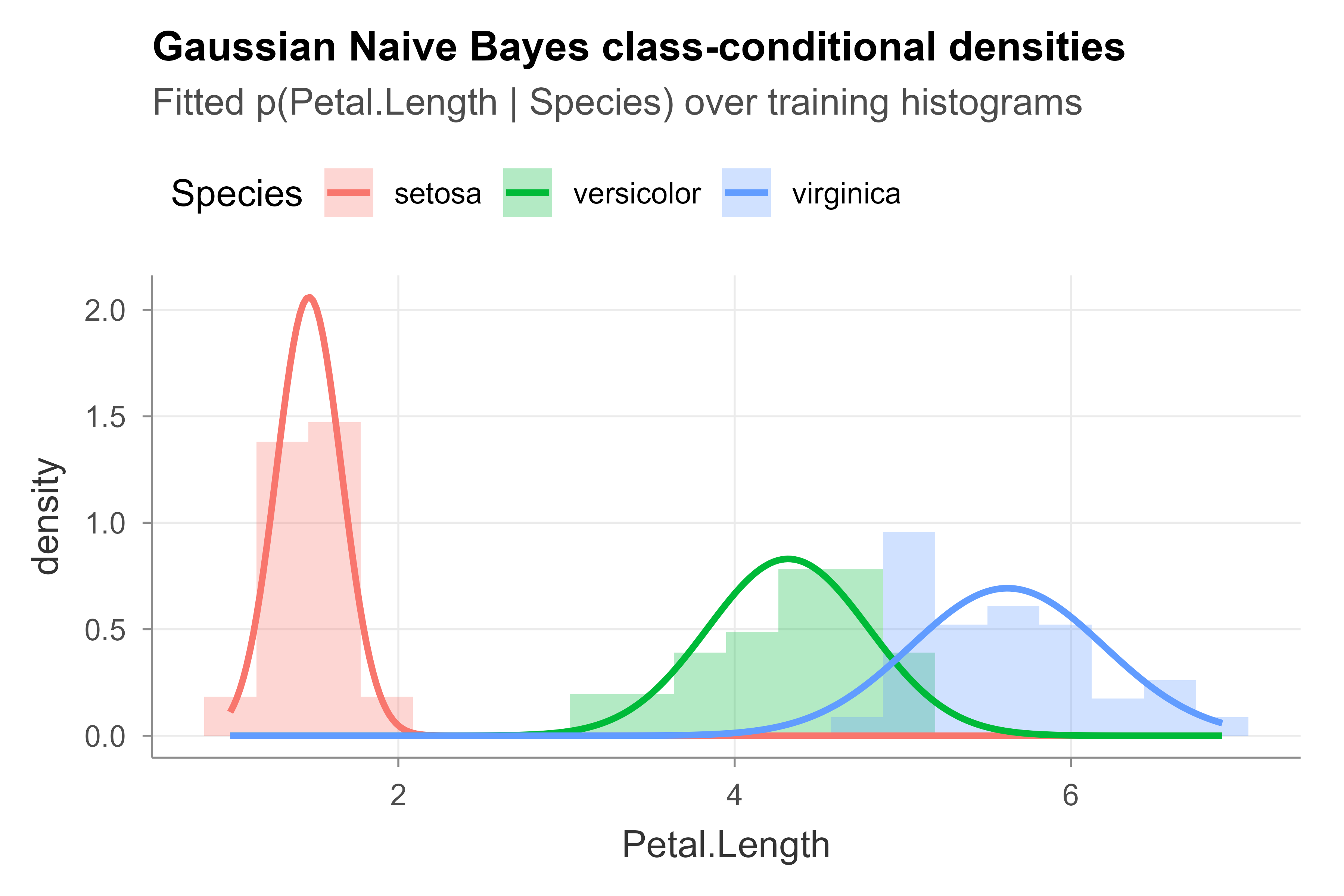
Each fitted curve sits squarely over its class’s histogram, which is why this feature is so informative. The slight overlap between the two larger-petaled species is exactly where the occasional misclassification in the confusion matrix comes from.
18.5.3 When the Naive Assumption Is Violated
The iris example flatters Naive Bayes because petal measurements are already fairly separable. To see the cost of the independence assumption directly, we now construct a case engineered to violate it. We simulate two Gaussian classes that share a strongly correlated covariance structure. Within each class the two features have correlation \(0.9\), so conditional independence is badly wrong.
Show code
m <- 400
Sigma <- matrix(c(1, 0.9, 0.9, 1), nrow = 2)
g1 <- mvrnorm(m, mu = c(0, 0), Sigma = Sigma)
g2 <- mvrnorm(m, mu = c(2, 2), Sigma = Sigma)

sim <- data.frame(
  x1 = c(g1[, 1], g2[, 1]),
  x2 = c(g1[, 2], g2[, 2]),
  y = factor(rep(c("A", "B"), each = m))
)

s_train <- sample(nrow(sim), floor(0.7 * nrow(sim)))
nb_corr <- naiveBayes(y ~ x1 + x2, data = sim[s_train, ])
pred_corr <- predict(nb_corr, sim[-s_train, ])
mean(pred_corr == sim$y[-s_train])
#> [1] 0.8541667
The classifier still separates the classes reasonably well, but its accuracy is lower than a method that models the within-class correlation (such as linear discriminant analysis, see Chapter 20, or logistic regression) would achieve here, because Naive Bayes treats the two highly redundant features as if each carried independent information.
18.5.4 Verifying the Gaussian-to-Logistic Weight Formula
The derivation in Section 18.4.3 claims that, with shared variances, the Gaussian Naive Bayes log-odds are linear in \(x\) with slope \(w_j = (\mu_{j1} - \mu_{j0})/\sigma_j^2\). We can confirm this numerically by computing the closed-form weights from the per-class moments and checking that they reproduce the model’s own log-odds on test points. We pool the variance across classes to match the shared-variance assumption.
Show code
d <- iris[iris$Species != "setosa", ]
d$y <- as.integer(d$Species == "virginica")  # 1 = virginica, 0 = versicolor
X <- as.matrix(d[, 1:4]); p <- ncol(X)

mu1 <- colMeans(X[d$y == 1, ]); mu0 <- colMeans(X[d$y == 0, ])
# pooled within-class variance per feature (shared-variance assumption)
v <- sapply(1:p, function(j)
  (sum((X[d$y == 1, j] - mu1[j])^2) + sum((X[d$y == 0, j] - mu0[j])^2)) / nrow(X))

prior <- mean(d$y)
w  <- (mu1 - mu0) / v
w0 <- log(prior / (1 - prior)) - sum((mu1^2 - mu0^2) / (2 * v))

# closed-form log-odds vs. a direct Gaussian-density computation
logodds_formula <- as.numeric(w0 + X %*% w)
logodds_direct <- log(prior/(1-prior)) + rowSums(
  dnorm(X, matrix(mu1, nrow(X), p, byrow = TRUE), matrix(sqrt(v), nrow(X), p, byrow = TRUE), log = TRUE) -
  dnorm(X, matrix(mu0, nrow(X), p, byrow = TRUE), matrix(sqrt(v), nrow(X), p, byrow = TRUE), log = TRUE))

max(abs(logodds_formula - logodds_direct))  # ~0 up to floating point
#> [1] 1.776357e-14
The maximum discrepancy is at the level of floating-point error, confirming that the per-feature Gaussian factors collapse exactly into the linear log-odds derived above.
18.6 Practical Notes
To close, here are the points that matter most when you actually deploy a Naive Bayes classifier, distilled into a checklist:
- Naive Bayes trains in a single pass over the data and predicts in time linear in the number of features, which makes it a strong baseline and a good choice when speed or memory is limited.
- It handles high-dimensional sparse inputs (such as text) gracefully, which is why the multinomial and Bernoulli variants remain standard text-classification baselines.
- The predicted class is usually more trustworthy than the predicted probability. Correlated features make Naive Bayes overconfident, so its probabilities often need recalibration (for example, Platt scaling or isotonic regression; see the probability calibration chapter, Chapter 86) before being used as risk scores.
- Always apply smoothing for count and binary features to avoid the zero-frequency problem. For continuous features, guard against zero or near-zero estimated variances, which produce unstable likelihoods.
- Decorrelating or pruning highly redundant features can help, since duplicated features are effectively double-counted under the independence assumption.
The single most common production mistake with Naive Bayes is using its raw probability outputs as if they were calibrated risk scores. Trust the predicted label; treat the predicted probability with suspicion until you have recalibrated it.
18.7 Further Reading
- Domingos and Pazzani (1997) on the optimality of Naive Bayes under zero-one loss.
- Ng and Jordan (2002) on the discriminative-generative comparison with logistic regression.
- Hastie, Tibshirani, and Friedman, The Elements of Statistical Learning, on generative classifiers and the bias-variance view.
- Manning, Raghavan, and Schutze, Introduction to Information Retrieval, on multinomial and Bernoulli Naive Bayes for text.
A generative classifier models how the data were generated, the full joint \(p(x, y)\), and then derives the posterior from it. This contrasts with a discriminative classifier such as logistic regression, which models \(p(y \mid x)\) directly and never bothers to describe how \(x\) arises. We return to this distinction in Section 18.4.3.↩︎
“Maximum a posteriori” means “the largest after seeing the data,” that is, the class with the highest posterior. It is the Bayesian counterpart of maximum likelihood, differing only by the inclusion of the prior \(p(y = c)\).↩︎
Subtracting \(m\) cancels in the ratio (it multiplies numerator and denominator by the same \(e^{-m}\)), so the probabilities are unchanged, but the largest exponent becomes \(e^0 = 1\), which keeps everything well within floating-point limits.↩︎