| Method | Adaptive | Scales with dimension | Uses past evaluations | Best when |
|---|---|---|---|---|
| Grid search | No | Very poorly (m^d) | No | 1-2 hyperparameters; full reproducibility |
| Random search | No | Well | No | Few key axes among many; strong default baseline |
| Bayesian optimization | Yes | Moderately | Yes | Evaluations very expensive; smooth low-dim space |
| Hyperband | Partly (via early stopping) | Well | Only to rank/prune | Training cost tunable by a resource budget |
84 Hyperparameter Optimization
Almost every model you fit in this book has two kinds of knobs. The first kind, the parameters, are learned from data by the fitting procedure itself: the coefficients of a linear model, the split points of a tree, the weights of a network. You do not set these by hand. The second kind, the hyperparameters, are the settings you choose before fitting begins and that the fitting procedure treats as fixed: the penalty strength \(\lambda\) in ridge or lasso, the number of trees and the learning rate in gradient boosting, the cost \(C\) and kernel width \(\gamma\) in a support vector machine, the number of neighbors \(k\) in nearest neighbors. The fitting procedure optimizes the parameters given the hyperparameters. Choosing the hyperparameters is a separate optimization problem sitting on top, and it is the subject of this chapter.
The reason this matters is that the gap between a poorly tuned model and a well tuned one is often larger than the gap between two different model families. A gradient boosting machine with a learning rate that is ten times too large can look worse than a plain linear regression, and the same machine tuned well can be the best thing on the table. So we need a principled way to search the space of hyperparameter settings, and we need to do it without fooling ourselves about how good the result really is.
Intuition
Think of hyperparameter optimization as a function you cannot write down. You feed it a setting, it hands back a validation score, and you have no formula and no gradient, only the ability to evaluate it (expensively, because each evaluation means fitting a model). The whole game is to find a good input using as few of these costly evaluations as possible.
Formally, let \(\boldsymbol{\lambda}\) denote a vector of hyperparameters living in a configuration space \(\Lambda\). For a setting \(\boldsymbol{\lambda}\) we train a model on a training set, then measure its quality on held-out data. Write the resulting (true, expected) generalization loss as a function \[ f(\boldsymbol{\lambda}) = \mathbb{E}_{(x,y)}\bigl[\, L\bigl(y,\, \hat{m}_{\boldsymbol{\lambda}}(x)\bigr)\,\bigr], \] where \(L\) is a loss (squared error, misclassification rate, negative log-likelihood) and \(\hat{m}_{\boldsymbol{\lambda}}\) is the model fitted under hyperparameters \(\boldsymbol{\lambda}\). We want \[ \boldsymbol{\lambda}^\star = \arg\min_{\boldsymbol{\lambda} \in \Lambda} f(\boldsymbol{\lambda}). \] We never observe \(f\) directly. We observe a noisy estimate of it, the cross-validation score, and each estimate costs one or more model fits. This is a black-box, derivative-free, expensive optimization problem. The methods in this chapter, grid search, random search, Bayesian optimization, and the bandit-style schedulers successive halving and Hyperband, are all answers to the same question: where should I spend my next evaluation?
This chapter assumes you know cross-validation (introduced in Chapter 1) and have met the models used as examples. By the end you will understand why random search beats grid search in more than two or three dimensions, how a Gaussian-process surrogate turns past evaluations into a map of where to look next, how Hyperband throws away bad configurations early to fit far more of them, and why nested cross-validation is the only honest way to report the score of a tuned model.
84.1 The configuration space and the loss surface
Before choosing a search method it helps to picture what we are searching over. Hyperparameters come in several flavors, and the shape of \(\Lambda\) drives the choice of method.
Some hyperparameters are continuous, such as a learning rate or a penalty \(\lambda\). These almost always matter most on a logarithmic scale: the difference between \(\lambda = 0.001\) and \(\lambda = 0.01\) is large, while the difference between \(\lambda = 10.001\) and \(\lambda = 10.01\) is nil. So we search \(\log \lambda\) on a uniform grid or with a uniform random draw, not \(\lambda\) itself. Some hyperparameters are integer-valued (number of trees, \(k\) in \(k\)-NN, tree depth). Some are categorical (which kernel, which split criterion). And some are conditional: the kernel width \(\gamma\) only exists if the kernel is radial-basis, so it is meaningless when the kernel is linear. A configuration space with conditional structure is a tree, not a box, which already rules out a naive product grid.
Key idea
Not all hyperparameters matter equally, and which ones matter is usually unknown in advance. This single empirical fact, the low effective dimensionality of most tuning problems, is the reason random search outperforms grid search, and it shapes everything that follows.
The function \(f(\boldsymbol{\lambda})\) is typically smooth in the continuous hyperparameters (small changes in \(\lambda\) give small changes in validation error) but it is noisy, because we estimate it by cross-validation on a finite sample. It can also be multimodal and have long flat regions. We have no gradient because the path from \(\boldsymbol{\lambda}\) to the score runs through a full model-fitting procedure. These features (smoothness, noise, no gradient, expensive evaluations) are exactly the regime that Bayesian optimization was built for, but the simpler methods are worth understanding first.
84.2 Grid search
The oldest and most transparent method is grid search. Pick a finite set of values for each hyperparameter and evaluate the model at every combination, the full Cartesian product. With two hyperparameters and ten values each, that is a \(10 \times 10 = 100\) point grid. Report the combination with the best cross-validation score.
Grid search has real virtues. It is trivial to implement, embarrassingly parallel (every grid point is independent), and completely reproducible. If the grid is coarse you can refine it around the winner and search again. For one or two important hyperparameters it is perfectly reasonable.
Its fatal flaw is the curse of dimensionality. The number of evaluations grows as the product of the per-axis resolutions. With \(d\) hyperparameters and \(m\) values each you face \(m^d\) fits. At \(m = 10\) and \(d = 5\) that is \(100{,}000\) model fits, which is hopeless if each fit takes a minute. Worse, the grid spends its budget uniformly across all axes even though, as noted above, only one or two axes usually matter. If you put ten grid values on an axis that turns out to be irrelevant, you have tried the same ten useful settings ten times over while wasting nine-tenths of your budget distinguishing values that do not affect the score.
Warning
Grid search couples your resolution on the important axes to your budget on the unimportant ones. Doubling resolution on every axis multiplies cost by \(2^d\). Beyond two or three hyperparameters, grid search is almost never the right tool.
84.3 Random search
The fix proposed by Bergstra and Bengio (2012) is disarmingly simple. Instead of a grid, draw each configuration’s hyperparameters independently at random from chosen distributions (uniform on a log scale for continuous penalties, uniform over the integer range for counts, uniform over levels for categoricals) and evaluate a fixed budget of \(n\) such random points. Keep the best.
Why does this beat a grid of the same size? Suppose only one of your \(d\) hyperparameters actually affects the score (a caricature, but close to the truth in many problems). A grid with \(m\) values per axis tries only \(m\) distinct values of the one important hyperparameter, no matter how large the total budget \(m^d\). Random search with the same budget of \(n = m^d\) points tries (with probability one) \(n\) distinct values of that important hyperparameter, because each draw is fresh on every axis. Random search automatically allocates more resolution to whichever axis happens to matter, without being told which one that is.
There is a clean probabilistic guarantee that makes random search attractive even when you know nothing about \(f\). Define the top \(p\) fraction of the configuration space as “good”, meaning a random draw lands in the good region with probability \(p\). After \(n\) independent draws, the probability that at least one of them is good is \[ \Pr(\text{at least one good in } n \text{ draws}) = 1 - (1 - p)^n. \] To make this probability at least \(1 - \delta\) we solve \((1-p)^n \le \delta\), giving \[ n \ \ge\ \frac{\log \delta}{\log(1 - p)}. \] For example, to have a \(95\%\) chance (\(\delta = 0.05\)) of landing in the top \(5\%\) (\(p = 0.05\)) of configurations, we need \(n \ge \log(0.05)/\log(0.95) \approx 58.4\), so \(59\) random evaluations suffice. Strikingly, this bound does not depend on the dimension \(d\) at all. It depends only on how large the good region is relative to the whole space.
Note
This guarantee is about hitting the good region of the space, not about finding the single best point. Random search is excellent at quickly getting you somewhere good and terrible at the last bit of polishing. That is exactly the gap Bayesian optimization fills.
84.4 Bayesian optimization
Grid and random search are non-adaptive: the points they evaluate do not depend on the results seen so far. That is wasteful, because once you have seen a few scores you have information about where good configurations might be. Bayesian optimization (Mockus 1978; Snoek, Larochelle, and Adams 2012) uses every past evaluation to decide the next one.
The recipe has two pieces: a surrogate model that approximates \(f\) and quantifies its own uncertainty, and an acquisition function that turns the surrogate into a recommendation for the next point to try.
84.4.1 The Gaussian-process surrogate
The standard surrogate is a Gaussian process (Chapter 7). A Gaussian process places a prior over functions such that any finite set of function values is jointly Gaussian. It is specified by a mean function \(\mu(\boldsymbol{\lambda})\), usually taken to be a constant, and a covariance (kernel) function \(k(\boldsymbol{\lambda}, \boldsymbol{\lambda}')\) that says how correlated the function values at two configurations are. A common choice is the squared-exponential kernel \[ k(\boldsymbol{\lambda}, \boldsymbol{\lambda}') = \sigma_f^2 \exp\!\left( -\frac{\lVert \boldsymbol{\lambda} - \boldsymbol{\lambda}' \rVert^2}{2 \ell^2} \right), \] where \(\ell\) is a length scale (how far you must move before the function changes appreciably) and \(\sigma_f^2\) is the signal variance.
Given \(t\) observed configurations \(\boldsymbol{\lambda}_1, \dots, \boldsymbol{\lambda}_t\) with (noisy) scores \(y_1, \dots, y_t\), collected in a vector \(\mathbf{y}\), the Gaussian process gives a closed-form posterior at any new configuration \(\boldsymbol{\lambda}\). Let \(\mathbf{k}(\boldsymbol{\lambda})\) be the vector of covariances between \(\boldsymbol{\lambda}\) and the observed points, \(\mathbf{K}\) the \(t \times t\) matrix of covariances among observed points, and \(\sigma_n^2\) the noise variance of an observation. Then the posterior mean and variance are \[ \mu_t(\boldsymbol{\lambda}) = \mathbf{k}(\boldsymbol{\lambda})^\top \bigl(\mathbf{K} + \sigma_n^2 \mathbf{I}\bigr)^{-1} \mathbf{y}, \] \[ \sigma_t^2(\boldsymbol{\lambda}) = k(\boldsymbol{\lambda}, \boldsymbol{\lambda}) - \mathbf{k}(\boldsymbol{\lambda})^\top \bigl(\mathbf{K} + \sigma_n^2 \mathbf{I}\bigr)^{-1} \mathbf{k}(\boldsymbol{\lambda}). \] The posterior mean \(\mu_t\) is our best guess of the score at \(\boldsymbol{\lambda}\), and the posterior standard deviation \(\sigma_t\) is how unsure we are. Near observed points \(\sigma_t\) is small; far from any observation it is large. This calibrated uncertainty is the engine of the whole method.
84.4.2 Acquisition functions
The surrogate gives a belief about \(f\) everywhere. An acquisition function \(\alpha(\boldsymbol{\lambda})\) scores how useful it would be to evaluate \(f\) at \(\boldsymbol{\lambda}\) next, balancing exploitation (go where the mean looks good) against exploration (go where the variance is high and we might be surprised). We then pick \(\boldsymbol{\lambda}_{t+1} = \arg\max_{\boldsymbol{\lambda}} \alpha(\boldsymbol{\lambda})\). Maximizing \(\alpha\) is cheap because it only touches the surrogate, not the real model.
Three acquisition functions are standard. Assume we are minimizing and let \(y^\star = \min_i y_i\) be the best (lowest) score seen so far. Write \(\mu = \mu_t(\boldsymbol{\lambda})\) and \(\sigma = \sigma_t(\boldsymbol{\lambda})\) for brevity, and let \(\phi\) and \(\Phi\) be the standard normal density and cumulative distribution function.
The probability of improvement is the chance the new point beats the incumbent: \[ \mathrm{PI}(\boldsymbol{\lambda}) = \Phi\!\left( \frac{y^\star - \mu - \xi}{\sigma} \right), \] where \(\xi \ge 0\) is a small margin that prevents the method from clustering greedily around the current best.
The expected improvement weights the probability of beating the incumbent by how much it beats it. With \(z = (y^\star - \mu - \xi)/\sigma\), \[ \mathrm{EI}(\boldsymbol{\lambda}) = (y^\star - \mu - \xi)\,\Phi(z) + \sigma\,\phi(z), \qquad \sigma > 0, \] and \(\mathrm{EI} = 0\) when \(\sigma = 0\). Expected improvement is the default workhorse: it has a closed form, needs no tuning constant beyond the optional \(\xi\), and naturally favors points that are either promising in mean or uncertain enough to surprise us.
The lower confidence bound (the minimization counterpart of the upper confidence bound) is the most explicit about the trade-off: \[ \mathrm{LCB}(\boldsymbol{\lambda}) = \mu - \kappa\, \sigma, \] and we minimize it. The constant \(\kappa > 0\) dials exploration: large \(\kappa\) chases uncertain regions, small \(\kappa\) exploits the mean. This form connects directly to the bandit ideas of Chapter 65: “optimism in the face of uncertainty” applied to a continuous search space.
Intuition
Expected improvement asks, “If I sample here, how much do I expect to improve on my best score so far?” It is large where the mean is good (likely improvement) and also where the variance is large (a small chance of a big improvement). That is the whole exploration/exploitation balance in one formula.
Bayesian optimization shines when evaluations are genuinely expensive (minutes to hours per fit), because fitting and maximizing the surrogate is cheap relative to one real evaluation. Its weaknesses are that the Gaussian process scales as \(O(t^3)\) in the number of evaluations \(t\), it struggles in very high dimensions, and it handles categorical and conditional spaces awkwardly. For those cases practitioners often switch the surrogate to a tree-structured Parzen estimator (Bergstra et al. 2011) or a random forest (Hutter, Hoos, and Leyton-Brown 2011).
84.5 Successive halving and Hyperband
Bayesian optimization is smart about which configuration to try next but still pays full price to evaluate each one. A different idea attacks the cost of evaluation itself. Many models can be trained at varying levels of fidelity controlled by a resource budget \(r\): number of boosting rounds, number of training epochs, or size of a data subsample. A configuration that is hopeless after a small budget is almost always still hopeless after a large one. So why pay full price to confirm it?
Successive halving (Jamieson and Talwalkar 2016) exploits this. Start with a large set of \(n\) randomly drawn configurations and a small per-configuration resource \(r\). Evaluate all \(n\) at budget \(r\), keep the best fraction \(1/\eta\) (typically \(\eta = 3\), so keep the top third), then multiply the surviving configurations’ budget by \(\eta\) and repeat. At each round you spend roughly the same total resource (fewer configurations, each given more), but you concentrate the budget on survivors. After a handful of rounds a single configuration remains, having been trained at the full budget, while the losers were eliminated cheaply.
The catch is a built-in trade-off governed by \(n\) for a fixed total budget \(B\): many configurations each started at a tiny budget (aggressive early stopping, risks killing a slow starter that would have won) versus few configurations each given a generous start (safe but explores less). You cannot know in advance which regime suits your problem.
Hyperband (Li et al. 2017) removes the guesswork by running successive halving as a subroutine across several values of the starting trade-off, called brackets. One bracket starts with very many configurations at a tiny budget (maximally aggressive). The next starts with fewer at a larger budget. The last bracket starts with a handful run to full budget, which is just random search with no early stopping at all. By hedging across brackets, Hyperband is robust: if early stopping helps, the aggressive brackets win; if it hurts, the conservative brackets cover you. The price is a small constant-factor overhead relative to the single best bracket you would have chosen with hindsight.
When to use this
Reach for successive halving and Hyperband when training cost scales with a tunable resource and when cheap, low-fidelity evaluations correlate with full-fidelity performance (true for most iterative learners, boosting and neural nets especially). They compose well with random sampling and, in modern systems, with Bayesian optimization choosing the configurations that each bracket starts from (the BOHB approach of Falkner, Klein, and Hutter 2018).
Table 84.1 summarizes how the four families compare on the dimensions that drive the choice in practice.
Table 84.1 shows the central trade-off: the methods that use past evaluations (Bayesian optimization) or prune cheaply (Hyperband) buy sample efficiency at the cost of more machinery, while random search buys robustness and simplicity at the cost of ignoring everything it has learned.
84.6 A runnable demo: grid versus random search
We now compare grid and random search head to head on a concrete tuning problem, using only base R and cross-validation. We tune a small regularized model with two hyperparameters and track the best score so far as a function of the number of evaluations, the standard way to read the efficiency of a search.
We use the mtcars data and an elastic-net-style penalized regression coded by hand so the demo depends on nothing beyond base R. The two hyperparameters are the penalty strength \(\lambda\) (searched on a log scale) and the mixing parameter \(\alpha \in [0, 1]\) that blends ridge (\(\alpha = 0\)) and a lasso-like penalty. The objective \(f(\boldsymbol{\lambda})\) is the cross-validated mean squared error.
Show code
set.seed(1)

# Design matrix (standardized predictors) and response from mtcars.
X <- scale(as.matrix(mtcars[, c("hp", "wt", "disp", "drat", "qsec")]))
y <- mtcars$mpg
n <- nrow(X)

# 5-fold cross-validated MSE for a penalized regression with an
# elastic-net-style penalty, fitted by coordinate-friendly ridge updates.
# We approximate the L1 part with a smooth surrogate so everything stays base R.
fit_predict_mse <- function(lambda, alpha, folds) {
  k <- length(unique(folds))
  errs <- numeric(k)
  p <- ncol(X)
  for (f in seq_len(k)) {
    tr <- folds != f
    te <- !tr
    Xtr <- X[tr, , drop = FALSE]
    ytr <- y[tr]
    # Effective per-coordinate penalty: ridge weight + lasso-like reweighting.
    # Ridge closed form with a diagonal penalty matrix P.
    pen <- lambda * ((1 - alpha) + alpha * 1.5)  # blend ridge/lasso strength
    P <- diag(pen, p)
    beta <- solve(t(Xtr) %*% Xtr + P, t(Xtr) %*% (ytr - mean(ytr)))
    pred <- X[te, , drop = FALSE] %*% beta + mean(ytr)
    errs[f] <- mean((y[te] - pred)^2)
  }
  mean(errs)
}

# Fixed fold assignment so grid and random search see the same CV splits.
folds <- sample(rep(seq_len(5), length.out = n))

objective <- function(log_lambda, alpha) {
  fit_predict_mse(exp(log_lambda), alpha, folds)
}
With the objective in hand we run both searches under the same total budget of evaluations so the comparison is fair. Grid search uses a \(6 \times 6\) grid over \((\log \lambda, \alpha)\); random search draws the same number of points uniformly from the same ranges.
Show code
budget <- 36
log_lambda_range <- c(-4, 4)   # lambda from ~0.018 to ~55
alpha_range      <- c(0, 1)

# --- Grid search: 6 x 6 Cartesian product ---
g <- 6
grid <- expand.grid(
  log_lambda = seq(log_lambda_range[1], log_lambda_range[2], length.out = g),
  alpha      = seq(alpha_range[1], alpha_range[2], length.out = g)
)
grid_scores <- mapply(objective, grid$log_lambda, grid$alpha)

# --- Random search: same number of points drawn uniformly ---
set.seed(42)
rand <- data.frame(
  log_lambda = runif(budget, log_lambda_range[1], log_lambda_range[2]),
  alpha      = runif(budget, alpha_range[1], alpha_range[2])
)
rand_scores <- mapply(objective, rand$log_lambda, rand$alpha)

# Best-score-so-far (running minimum of CV MSE) for each method.
best_so_far <- function(scores) cummin(scores)
grid_curve <- best_so_far(grid_scores)
rand_curve <- best_so_far(rand_scores)

# Report the winners.
data.frame(
  method = c("grid", "random"),
  best_cv_mse = round(c(min(grid_scores), min(rand_scores)), 3),
  best_lambda = round(c(exp(grid$log_lambda[which.min(grid_scores)]),
                        exp(rand$log_lambda[which.min(rand_scores)])), 3),
  best_alpha  = round(c(grid$alpha[which.min(grid_scores)],
                        rand$alpha[which.min(rand_scores)]), 3)
)
#>   method best_cv_mse best_lambda best_alpha
#> 1   grid       7.474       0.449      1.000
#> 2 random       7.434       1.165      0.436
To make the comparison less dependent on a single lucky or unlucky random seed, we repeat random search over many seeds and average the best-so-far curves. This is the honest way to compare a stochastic method against a deterministic one.
Show code
n_rep <- 200
rep_curves <- matrix(NA_real_, nrow = n_rep, ncol = budget)
for (r in seq_len(n_rep)) {
  set.seed(1000 + r)
  rl <- runif(budget, log_lambda_range[1], log_lambda_range[2])
  ra <- runif(budget, alpha_range[1], alpha_range[2])
  rs <- mapply(objective, rl, ra)
  rep_curves[r, ] <- cummin(rs)
}
rand_curve_mean <- colMeans(rep_curves)
The figure plots the best cross-validated MSE found so far against the number of evaluations spent, for grid search and for the averaged random search.
Show code
q10 <- apply(rep_curves, 2, quantile, 0.10)
q90 <- apply(rep_curves, 2, quantile, 0.90)

plot(seq_len(budget), grid_curve, type = "l", lwd = 2,
     ylim = range(c(grid_curve, q10, q90)),
     xlab = "Number of evaluations", ylab = "Best CV MSE so far",
     main = "Grid vs random search: best score so far")
polygon(c(seq_len(budget), rev(seq_len(budget))), c(q90, rev(q10)),
        col = rgb(0.2, 0.4, 0.8, 0.15), border = NA)
lines(seq_len(budget), rand_curve_mean, lwd = 2, lty = 2, col = "navy")
legend("topright",
       legend = c("Grid search", "Random search (mean of 200)", "Random 10-90% band"),
       lwd = c(2, 2, 8), lty = c(1, 2, 1),
       col = c("black", "navy", rgb(0.2, 0.4, 0.8, 0.3)), bty = "n")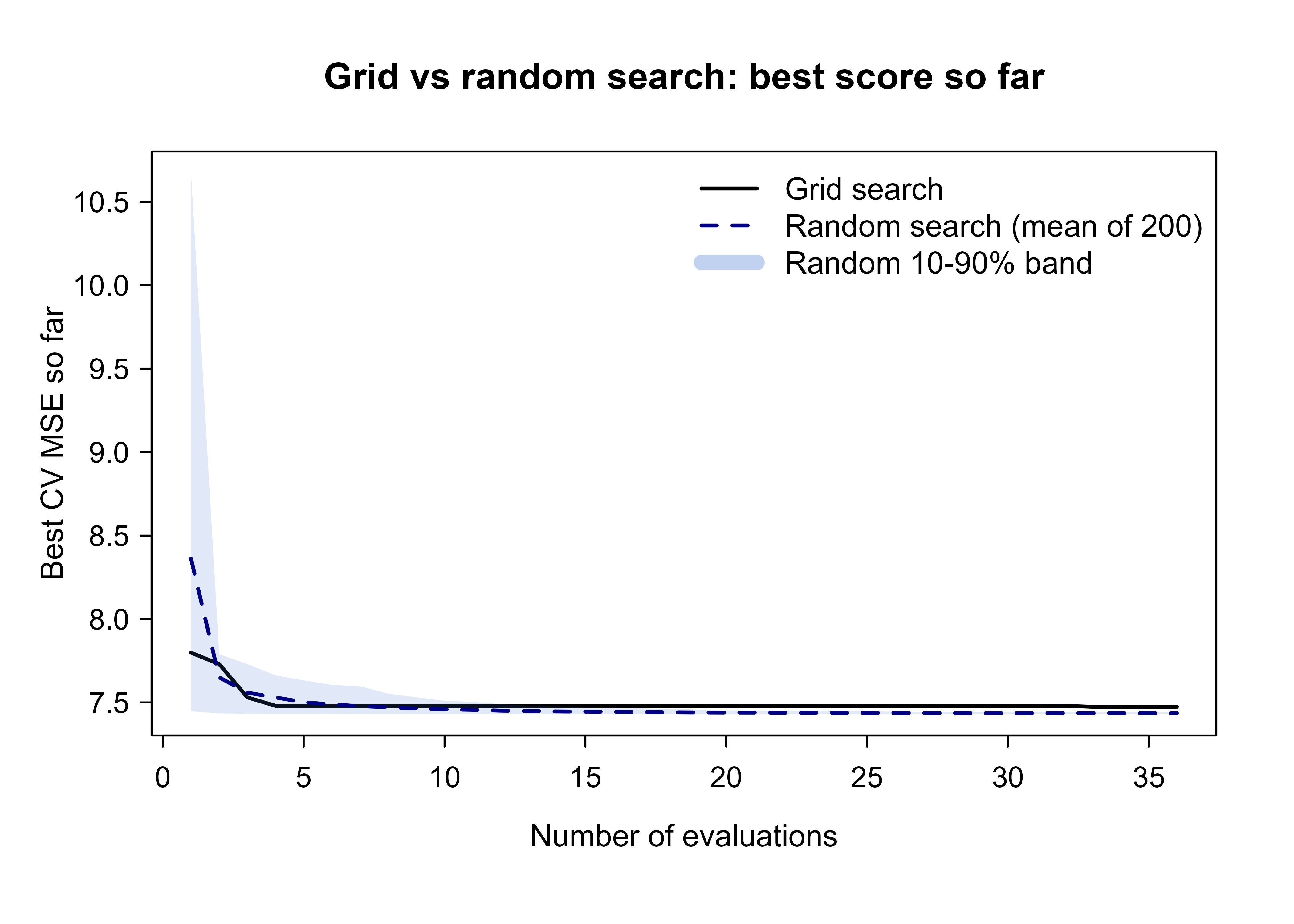
Figure 84.1 shows what the theory predicts. With only two hyperparameters the advantage of random search is modest, because a \(6 \times 6\) grid already resolves both axes reasonably. The gap widens dramatically as dimension grows, since the grid’s resolution per important axis collapses while random search keeps drawing fresh values on every axis. The shaded band also makes the cost of randomness visible: any single random run can be lucky or unlucky, which is why averaging (or simply using a generous budget) matters.
Note
This demo hand-rolls a penalized regression to stay in base R. In real work you would tune a proper model: glmnet for the elastic net, xgboost for boosting (Chapter 12), e1071::svm for a support vector machine (Chapter 19), wrapped in a cross-validation loop or a framework such as tidymodels (Chapter 90). The search logic (objective returns a CV score, track best-so-far) is identical.
84.7 Nested cross-validation: not fooling yourself
There is a subtle and very common mistake hiding in everything above. Suppose you run a search, pick the configuration with the best cross-validation score, and then report that best score as your model’s performance. That number is optimistically biased. By searching over many configurations and reporting the best one, you have let the validation folds influence model selection, so the selected score has been partly fitted to the validation data. The more configurations you try, the worse the bias, by the same logic as the maximum of many noisy estimates exceeding their common mean.
Warning
The cross-validation score of the configuration you selected is not an unbiased estimate of how that configuration will perform on new data. Reporting it as your final performance number is one of the most common errors in applied machine learning, and it inflates results in proportion to how hard you searched.
The fix is nested cross-validation. Use two nested loops. The outer loop splits the data into folds purely for evaluation. For each outer fold, hold it out, and on the remaining data run a complete inner cross-validation to select hyperparameters. Then fit the selected configuration on all of the outer-training data and score it once on the held-out outer fold. The outer fold was never seen by the hyperparameter search, so its score is an honest estimate of the whole tuning-plus-fitting procedure. Average the outer-fold scores to report performance.
Schematically, with \(K\) outer folds and \(J\) inner folds: \[ \text{for each outer fold } i: \quad \hat{\boldsymbol{\lambda}}_i = \arg\min_{\boldsymbol{\lambda}} \; \mathrm{CV}^{\text{inner}}_{J}\bigl(\boldsymbol{\lambda}; \,\mathcal{D} \setminus \mathcal{D}_i\bigr), \qquad e_i = L\bigl(\mathcal{D}_i; \, \hat{m}_{\hat{\boldsymbol{\lambda}}_i} \text{ fit on } \mathcal{D} \setminus \mathcal{D}_i\bigr), \] and the reported performance is \(\frac{1}{K}\sum_{i=1}^{K} e_i\). Note that the selected \(\hat{\boldsymbol{\lambda}}_i\) may differ across outer folds, and that is fine: nested CV estimates the performance of the procedure, not of one fixed configuration. Once you trust the procedure, you run the inner search one final time on all the data to choose the configuration you ship.
The following demo measures the bias directly. It compares the (optimistic) best inner-CV score against the (honest) nested-CV score for our tuning task.
Show code
set.seed(7)

# A small random search returning best inner-CV score AND the chosen config.
inner_search <- function(idx, budget = 20) {
  Xs <- X[idx, , drop = FALSE]; ys <- y[idx]
  m <- length(idx)
  inner_folds <- sample(rep(seq_len(5), length.out = m))
  cv_mse <- function(log_lambda, alpha) {
    k <- 5; errs <- numeric(k); p <- ncol(Xs)
    for (f in seq_len(k)) {
      tr <- inner_folds != f; te <- !tr
      pen <- exp(log_lambda) * ((1 - alpha) + alpha * 1.5)
      beta <- solve(t(Xs[tr, ]) %*% Xs[tr, ] + diag(pen, p),
                    t(Xs[tr, ]) %*% (ys[tr] - mean(ys[tr])))
      pred <- Xs[te, , drop = FALSE] %*% beta + mean(ys[tr])
      errs[f] <- mean((ys[te] - pred)^2)
    }
    mean(errs)
  }
  ll <- runif(budget, -4, 4); aa <- runif(budget, 0, 1)
  sc <- mapply(cv_mse, ll, aa)
  j <- which.min(sc)
  list(score = sc[j], log_lambda = ll[j], alpha = aa[j])
}

# Fit a configuration on a training index, score on a test index.
fit_score <- function(tr_idx, te_idx, log_lambda, alpha) {
  p <- ncol(X)
  pen <- exp(log_lambda) * ((1 - alpha) + alpha * 1.5)
  beta <- solve(t(X[tr_idx, ]) %*% X[tr_idx, ] + diag(pen, p),
                t(X[tr_idx, ]) %*% (y[tr_idx] - mean(y[tr_idx])))
  pred <- X[te_idx, , drop = FALSE] %*% beta + mean(y[tr_idx])
  mean((y[te_idx] - pred)^2)
}

# Optimistic estimate: search on all data, report the best inner-CV score.
optimistic <- inner_search(seq_len(n), budget = 20)$score

# Honest estimate: nested CV with 5 outer folds.
outer_folds <- sample(rep(seq_len(5), length.out = n))
outer_err <- numeric(5)
for (i in seq_len(5)) {
  te_idx <- which(outer_folds == i)
  tr_idx <- which(outer_folds != i)
  best <- inner_search(tr_idx, budget = 20)
  outer_err[i] <- fit_score(tr_idx, te_idx, best$log_lambda, best$alpha)
}
nested <- mean(outer_err)

data.frame(
  estimate = c("optimistic (best inner-CV)", "nested CV (honest)"),
  mse = round(c(optimistic, nested), 3)
)
#>                     estimate   mse
#> 1 optimistic (best inner-CV) 8.176
#> 2         nested CV (honest) 9.609
The optimistic number is the one you would proudly report if you skipped nesting; the nested number is closer to what you will actually see in production. On this tiny dataset the gap is modest, but it grows with the number of configurations searched and shrinks the sample size, exactly the regime where careful evaluation matters most.
84.8 Practical guidance and pitfalls
A workable default workflow looks like this. Start with random search over sensibly chosen ranges (log scale for anything multiplicative) to get a strong baseline cheaply and to learn which hyperparameters actually move the score. If evaluations are expensive and the space is low-dimensional and continuous, switch to Bayesian optimization to polish. If training cost scales with a resource (epochs, rounds, data fraction), wrap the whole thing in Hyperband so bad configurations die young. Always report performance with nested cross-validation, or with a clean held-out test set that the search never touched.
Several traps catch people.
Warning
Search ranges matter more than the search algorithm. A clever optimizer over a badly chosen range loses to random search over a good one. Set ranges on the right scale (log for penalties and learning rates) and wide enough to bracket the optimum, then check that the winner does not sit on a boundary, which signals the range was too narrow.
The first trap is leaking the test set into tuning. Any preprocessing fitted on the full data (scaling, feature selection, imputation) before the cross-validation split leaks information from validation folds into training. Fit all preprocessing inside the cross-validation loop, on training folds only.
The second trap is comparing methods on different budgets. Random search with \(200\) evaluations will beat grid search with \(36\), but that says nothing about the methods. Hold the total evaluation budget fixed when comparing, as the demo does.
The third trap is ignoring the noise in the objective. Cross-validation scores are random. Two configurations whose CV scores differ by less than the fold-to-fold standard error are statistically tied; picking the nominally best one is partly chance. Prefer the simplest configuration among the statistical ties (largest penalty, fewest trees), which also tends to generalize better, an instance of the one-standard-error rule.
The fourth trap is forgetting reproducibility and cost. Log every configuration and its score, set seeds, and record wall-clock cost per evaluation. Hyperparameter optimization can quietly consume more compute than all your model development combined, so treat the budget as a first-class quantity to be spent deliberately.
A last point on dimensionality: most of the gain comes from a handful of hyperparameters. Before launching a large search, fix the unimportant hyperparameters at sensible defaults and tune only the two or three that the literature (or a quick random-search probe) says matter. A focused search over the right axes beats a sprawling one over all of them.
84.9 Further reading
Bergstra and Bengio (2012) is the readable, decisive paper showing why random search beats grid search and is the place to start. For Bayesian optimization, Snoek, Larochelle, and Adams (2012) is the practical machine-learning entry point, Shahriari et al. (2016) is a thorough review, and Rasmussen and Williams (2006) is the standard reference on the Gaussian processes that power the surrogate. The original expected-improvement idea traces to Mockus (1978) and to Jones, Schonlau, and Welch (1998). For the bandit-style schedulers, Jamieson and Talwalkar (2016) introduce successive halving and Li et al. (2017) introduce Hyperband, with Falkner, Klein, and Hutter (2018) combining it with Bayesian optimization. Bergstra et al. (2011) and Hutter, Hoos, and Leyton-Brown (2011) give the tree-Parzen and random-forest surrogates that handle conditional and categorical spaces. On honest evaluation, Cawley and Talbot (2010) document the optimistic bias of non-nested tuning and motivate nested cross-validation. Bischl et al. (2023) survey the modern landscape and practical defaults.