Imagine you are handed a spreadsheet of customers, with no labels telling you who is who, and someone asks you to find the “natural groups” hiding inside it. Maybe there is a cluster of frequent, big spenders, another of occasional bargain hunters, and a third of people who signed up once and never returned. Nobody told you these groups exist or what to call them. Your job is to let the data reveal them. That is the goal of cluster analysis: discovering subgroups in a set of features when no answer key is provided.
Cluster analysis is a relatively large set of techniques used for finding subgroups, clusters, or segments in a set of features. The guiding idea is simple once you state it plainly. We first decide on some way to measure how similar or dissimilar two observations are, and we then try to form groups that are homogeneous, so that observations in a subgroup are more similar to each other than to other observations not in the subgroup. Everything else in this chapter is a way of making that one sentence precise and computable.
Because there is no outcome variable telling us the “right” grouping, cluster analysis belongs to unsupervised learning (Chapter 22). This is what separates it from classification methods you may already know. It is worth pausing on that contrast, because both families of methods sort observations into categories, but they do so for different reasons and with different information. Table 23.1 lines up cluster analysis against discriminant analysis, a supervised cousin.
Table 23.1: Comparison of cluster analysis and discriminant analysis, highlighting that clustering is unsupervised and groups by closeness, while discriminant analysis is supervised and classifies by the differences between known groups.
Cluster Analysis
Discriminant Analysis
Under framework
Unsupervised Learning
Supervised Learning
Dependent variable (category)
No
Yes
Classification rule based on
Closeness
Difference
Both discriminant analysis (Chapter 20) and cluster analysis are used to classify, but the resemblance ends there. Discriminant analysis is handed labeled examples and learns rules that exploit the differences between known groups; clustering is handed unlabeled data and must invent the groups using nothing but closeness.
In this chapter you will learn how clustering puts that intuition on a firm footing. We start with how to measure proximity between observations, since every clustering method rests on that choice. We then look at the two best known families of algorithms. K-means clustering partitions observations into a number of clusters you choose in advance. Hierarchical clustering builds a whole tree of nested groupings, so you can decide on the number of clusters after looking at the structure. Along the way we will see the variants K-medoids (a more robust relative of K-means) and the different “linkage” rules that give hierarchical clustering its flavor.
A few framing points are worth keeping in mind as we go.
We can cluster the observations to find subgroups of observations, or transpose the problem and cluster the features to find subgroups of features. The machinery is the same; only what plays the role of “object” changes.
Critical to all clustering approaches is the choice of distance, proximity, or dissimilarity measure between two objects. Change that measure and you can change the answer, so we treat it first and treat it carefully.
Key idea
Clustering does not find the “true” groups in some objective sense. It finds the groups implied by the similarity measure and algorithm you chose. The honest question is never “what are the clusters?” but “what are the clusters under these assumptions?”
23.1 Proximity Matrices
Since clustering is built entirely on the notion of “alike” versus “different,” our first task is to make that notion numerical. It is convenient to represent the data in terms of proximity (alikeness or affinity), which can be expressed either as similarity or as dissimilarity. The distinction is just a matter of direction: a similarity measure increases as two objects become more alike, while a dissimilarity measure decreases as two objects become more alike. Euclidean distance is the familiar example of a dissimilarity measure, since two points sitting on top of each other have distance zero.
To use dissimilarity as the foundation for an algorithm, we want it to behave like a sensible notion of distance. Formally, given two \(p\)-dimensional objects \(x_i\) and \(x_i'\), a dissimilarity measure \(d_{ii'}\) satisfies:
\(d_{ii'} \ge 0 \forall x_i, x_i'\)
\(d_{ii'} = 0\) iff \(x_i = x_i'\)
\(d_{ii'} = d_{i'i}\)
In words, dissimilarities are never negative, two objects are at distance zero exactly when they are identical, and the dissimilarity from \(i\) to \(i'\) is the same as from \(i'\) to \(i\). A measure that satisfies all of these conditions is said to be a semi-metric. If it further satisfies the triangle inequality, \(d_{ii'} \le d_{ik} + d_{i'k}\), then it is said to form a metric.1
Once we have a dissimilarity measure, we apply it to every pair of observations and collect the results. We typically form the \(n \times n\) proximity matrix, \(\mathbf{D}\), which in the case of a dissimilarity measure has \((i,j)\)th element given by \(d_{ij}\). This single matrix is the input that most clustering algorithms actually consume, which is a useful thing to notice: the algorithms never see your raw data directly, only the pairwise dissimilarities you computed from it.
Note
Because algorithms operate on \(\mathbf{D}\) rather than on the raw features, two completely different datasets that happen to produce the same proximity matrix will be clustered identically. All of your modeling choices about what “similar” means get baked into \(\mathbf{D}\) before any clustering begins.
23.1.1 Dissimilarities based on Attributes
How do we build the dissimilarity between two whole observations out of their individual features? The usual recipe is to score each attribute separately and then add up the scores. In general, we can define the dissimilarity by summing across the \(p\) attributes (that is, with equal weighting):
Here \(d_j\) measures dissimilarity on attribute \(j\) alone. A very common choice for that per-attribute term is squared distance,
\[
d_j(x_{ij}, x_{i'j}) = (x_{ij} - x_{i'j})^2
\]
which, summed over attributes, gives the squared Euclidean distance you already know. This default is reasonable for quantitative variables, but it quietly assumes a lot, and three issues come up in practice.
We may wish to use more general distance measures.
We may have categorical variables, which have no natural notion of subtraction.
We may wish to weight the attributes differently.
Each of these has a standard fix.
For the first, a general class of dissimilarities is the Minkowski metric,
which contains familiar distances as special cases: \(\lambda = 2\) is Euclidean distance, and \(\lambda = 1\) is the so-called Manhattan or city-block distance.2
The second issue, categorical variables, splits into two cases depending on whether the categories have an order. Consider first the situation where we have ordinal variables (categorical variables that have order, such as “small, medium, large”). Typically one converts these to a numerical value and then uses a quantitative metric. For example, if we have \(M\) ordinal values, we can replace them with \((i - 1/2)/M\) for \(i = 1, \dots, M\), spreading the categories evenly across the unit interval. For unordered categorical (nominal) variables, there is no order to exploit, so the degree of difference between pairs of values must be specified directly. These values are chosen in a way that maintains the symmetric nature of the dissimilarity matrix.
The third issue is weighting, and it is more subtle than it first appears. It is common to weight the elements of the discrepancy function differently depending on the attribute:
where \(w_j\) is a weight assigned to the \(j\)-th attribute. The natural instinct is that giving every attribute the same weight treats them all “equally,” but that instinct is wrong. As discussed in (Hastie, Friedman, and Tibshirani 2001, 14.3.3), setting the \(w_j\) to the same value for each variable does not necessarily give all of the attributes equal influence, because a variable that varies over a large range will dominate one that varies over a small range. They show that setting \(w_j\) proportional to \(1/\bar{d}_j\), where
gives all attributes equal influence. The twist is that equal influence is not always what you want, since the attribute that happens to vary the most may be precisely the one that carries the signal about the subgroups.
Warning
Standardizing or equalizing the influence of variables is a modeling decision, not a cleanup step. Forcing every feature to contribute equally can wash out the very feature that distinguishes the groups. Decide based on what you know about the problem, not by reflex.
23.2 Combinatorial Cluster Algorithms
We now have a way to measure dissimilarity. The next question is how to turn those dissimilarities into an actual assignment of observations to groups. The cleanest way to state the problem is combinatorial: think of it purely as choosing a label for each observation so as to make groups internally tight.
Let each observation be uniquely labeled by an integer \(i \in \{1, \dots, n\}\). A pre-specified number of clusters \(K<n\) is then assumed, and each cluster is labeled by an integer \(k \in \{ 1, \dots, K \}\). Each observation is assigned to one unique cluster. The assignment is characterized by an encoder, \(k = C(i)\), which assigns the \(i\)-th observation to the \(k\)-th cluster. We seek an encoder based on the dissimilarities \(d(x_i, x_i')\) between every pair of observations.
To choose among encoders, we have to specify some loss function that we would like the clustering to minimize. A natural one is the within-cluster point scatter,
which measures the extent to which observations assigned to the same cluster tend to be close to one another. We would like this to be small, since tight clusters are exactly the goal. Its mirror image is the between-cluster point scatter,
which is large when observations assigned to different clusters are far apart, that is, when the clusters are well separated. These two quantities are not independent. Their sum is the total point scatter,
which is constant given the data, independent of the cluster assignment, since it just sums dissimilarity over every pair regardless of labels.
This decomposition has a tidy consequence. Because \(T\) is fixed, pushing \(W(C)\) down automatically pulls \(B(C)\) up: minimizing \(W(C)\) is equivalent to maximizing \(B(C)\). We only ever have to optimize one of them.
To see that \(T = W(C) + B(C)\) holds for any assignment \(C\), fix a pair \((i, i')\) and ask which of the two sums it lands in. Every ordered pair appears exactly once in the double sum defining \(T\). If \(C(i) = C(i')\) the pair contributes to \(W(C)\), since the inner sums of \(W(C)\) range over pairs in the same cluster; if \(C(i) \neq C(i')\) it contributes to \(B(C)\). The two cases are mutually exclusive and exhaustive, so summing \(W(C)\) and \(B(C)\) recovers every pair once, which is exactly \(T\). Nothing about this argument used the form of \(d\), so the decomposition is purely combinatorial and holds for any dissimilarity.
Why the count is intractable
The number of distinct ways to partition \(n\) objects into exactly \(K\) nonempty groups is the Stirling number of the second kind, \[
S(n, K) = \frac{1}{K!} \sum_{j=0}^{K} (-1)^j \binom{K}{j} (K-j)^n .
\] For fixed \(K\) this grows like \(K^n / K!\), so the search space is exponential in \(n\). Even \(S(19, 4) \approx 1.1 \times 10^{10}\), which already rules out enumeration. This is why every practical method below is a greedy or iterative heuristic that returns a local optimum, and why K-means clustering (minimizing \(W(C)\) for squared Euclidean \(d\)) is in fact NP-hard in general, both when \(K\) is part of the input and even for \(K = 2\) in general dimension.
Intuition
The total amount of “spread” in your data is a fixed budget. Clustering does not reduce that spread; it only decides how much of it sits inside groups versus between them. Good clusters keep the within-group share small, which is the same as keeping the between-group share large.
In principle, one could solve this optimization problem exactly by considering every possible combination of observations and cluster assignments, then keeping the best. But the number of ways to partition \(n\) points into \(K\) groups grows astronomically, so such combinatorial algorithms are computationally prohibitive for most real-world datasets.3 In practice we settle for less: iterative descent algorithms that start from some assignment and improve it step by step, converging to a local optimum rather than the global one. The next two sections are exactly such algorithms.
23.2.1 K-Means Clustering
The K-means algorithm is one of the most popular and useful clustering algorithms, and it is the workhorse you are most likely to reach for first. It is typically used when all the variables are quantitative, and it commits to squared Euclidean distance as the dissimilarity metric:
This choice is not arbitrary; it is what lets the algorithm be so simple. With squared Euclidean distance, the within-cluster scatter can be rewritten in a form built around cluster means:
where \(\bar{x}_k = (\bar{x}_{1k}, \dots, \bar{x}_{pk})\) is the mean vector associated with the \(k\)-th cluster and \(n_k = \sum_{i=1}^n I(C(i)=k)\) is the number of points in cluster \(k\). The payoff is the right-hand side: minimizing \(W(C)\) amounts to assigning the \(n\) observations to the \(K\) clusters so that the within-cluster average dissimilarity between each observation and its cluster mean is as small as possible. In other words, the cluster mean (the centroid) is the natural “center” to measure against, and K-means simply alternates between computing centers and reassigning points to the nearest one.
23.2.1.1 Deriving the centroid identity
The collapse from a double sum over pairs to a single sum against the mean is the algebraic heart of K-means, so it is worth doing explicitly. The key is the following identity for any cluster \(k\) with \(n_k\) members:
Now sum over all ordered pairs \(i, i'\) in cluster \(k\). The first term gives \(n_k \sum_{C(i)=k} \|x_i - \bar{x}_k\|^2\) because the index \(i'\) is free and runs over \(n_k\) values; the second term gives the same quantity by symmetry. The cross term vanishes:
since \(\sum_{C(i)=k}(x_i - \bar{x}_k) = \sum_{C(i)=k} x_i - n_k \bar{x}_k = 0\) by the definition of the mean. Collecting terms, \(\sum_i \sum_{i'} \|x_i - x_{i'}\|^2 = 2 n_k \sum_i \|x_i - \bar{x}_k\|^2\), which is Equation 23.1. Summing over \(k\) gives the displayed form of \(W(C)\) above.
23.2.1.2 Why the mean is optimal, and Lloyd’s algorithm
A second fact justifies recomputing the mean at every iteration. For a fixed set of points \(S\), the point \(m\) minimizing the sum of squared Euclidean distances is the mean:
This follows by differentiating: \(\nabla_m \sum_{x \in S} \|x - m\|^2 = -2 \sum_{x \in S}(x - m) = 0\) gives \(m = \frac{1}{|S|}\sum_{x \in S} x\), and the objective is strictly convex in \(m\) (Hessian \(2|S| I \succ 0\)), so this stationary point is the unique global minimizer.
Putting Equation 23.2 together with the obvious fact that, holding the centroids fixed, assigning each point to its nearest centroid minimizes the objective over assignments, exposes K-means as block coordinate descent on the joint objective
Lloyd’s algorithm alternates the two exact minimizations: the assignment step minimizes \(J\) over \(C\) with \(\{m_k\}\) fixed, and the update step minimizes \(J\) over \(\{m_k\}\) with \(C\) fixed. Because each step is an exact minimization over one block, \(J\) is nonincreasing across iterations:
Since \(J \ge 0\) is bounded below and there are only finitely many distinct assignments \(C\) (at most \(K^n\)), the monotone sequence of objective values must stabilize, and the algorithm terminates in a finite number of iterations at a partition that is a local optimum (no single reassignment or recentering lowers \(J\)). This is exactly the convergence claim made informally above. It is not, however, a global optimum: the result depends on the initialization, which motivates multiple random starts.
Local optima and a smarter start
Uniformly random initial assignments can place all seeds in one region and leave genuine clusters merged. The k-means++ seeding rule of Arthur and Vassilvitskii samples the first center uniformly, then samples each subsequent center with probability proportional to its squared distance to the nearest already-chosen center (so far-away points are favored). This spreads seeds out and yields the guarantee \(\mathbb{E}[J_{\text{k-means++}}] \le 8(\ln K + 2)\, J_{\text{opt}}\), an \(O(\log K)\) approximation in expectation before any Lloyd iterations are even run. In R, kmeans() does not implement k-means++ directly, but combining several random starts via nstart is the practical substitute, and packages such as flexclust offer k-means++ seeding.
23.2.1.3 Cost, scaling, and failure modes
One Lloyd iteration costs \(O(nKp)\): each of \(n\) points is compared to \(K\) centroids in \(p\) dimensions, and the centroid update is a single \(O(np)\) pass. With \(I\) iterations the total is \(O(nKpI)\), which is linear in \(n\) and is why K-means scales to large datasets where the \(O(n^2)\) proximity matrix of the combinatorial view would be prohibitive. The memory footprint is \(O(np + Kp)\), since the full \(\mathbf{D}\) is never formed.
Three failure modes follow directly from the assumptions baked into Equation 23.3.
The squared norm makes each cluster an isotropic Gaussian-like ball in the chosen scale, so K-means implicitly assumes clusters of similar size, similar spread, and roughly spherical shape. Elongated, curved, or density-varying clusters (two concentric rings, say) are split incorrectly no matter how many restarts you use.
Squared distance squares the influence of outliers, so a single far point can drag a centroid and corrupt an entire cluster. This is the robustness argument for K-medoids.
Because the objective decreases monotonically in \(K\) (more centroids can only reduce \(J\), reaching \(J = 0\) when \(K = n\)), \(J\) alone cannot choose \(K\); you need an external criterion (see Section 23.3).
Randomly assign a number (\(1 \to K\)) to each of the observations. These are the initial cluster assignments.
Iterate until the cluster assignments stop changing:
For each of the \(K\) clusters, compute the cluster centroid. The \(k\)-th cluster centroid is the vector of the \(p\) feature means for the observations in the \(k\)-th cluster.
Assign each observation to the cluster whose centroid is closest, where closest is defined by Euclidean distance.
Each pass makes the within-cluster scatter no worse, which is why the procedure is guaranteed to settle down. Two practical points deserve emphasis.
The number of clusters \(K\) is yours to choose, and it genuinely matters: ask for three clusters and you get three, whether or not three is meaningful. The algorithm will not warn you that a different \(K\) tells a cleaner story.
Although the K-means algorithm is guaranteed to converge, it is not guaranteed to converge to the global minimum. Because it finds a local minimum that depends on the random starting assignment, we should run the algorithm several times from different initial cluster assignments and keep the best result, meaning the one with the smallest value of the objective function \(W(C)\).
Tip
Always run K-means with multiple random starts and report the best. A single run can land in a poor local optimum that looks fine until you compare it against a few others. Most software exposes this as an nstart-style argument; set it to a number like 20 or 50 rather than leaving it at 1.
23.2.2 K-Medoids Clustering
K-means is fast and intuitive, but it is wedded to squared Euclidean distance and to using the mean as a cluster center, and the mean is sensitive to outliers and undefined for non-numeric data. K-medoids loosens both restrictions. The key observation is that as long as you can construct a proximity matrix representing the dissimilarity between any two observations, this type of algorithm can be used with any dissimilarity measure you like, not just Euclidean distance. The trick is to insist that each cluster’s center be an actual observation (a medoid) rather than an abstract mean.
Then \(m_k = x_{i_k^*}, k = 1, 2, \dots, K\) are the current estimates of the cluster centers.
Given a current set of cluster centers \(\{m_1, \dots, m_K\}\), minimize the total error by assigning each observation to the closest current cluster center:
Iterate steps 1 and 2 until the assignments do not change.
When to use this
Reach for K-medoids instead of K-means when your dissimilarity is not Euclidean (for example, you only have a precomputed distance matrix), when outliers would distort an arithmetic mean, or when you want each cluster represented by a real, interpretable example rather than an average point. The cost is more computation, since finding the medoid means searching within each cluster.
The objective being minimized is the total dissimilarity to the assigned medoid,
with the constraint that each center is one of the observations. The same block-descent argument as for K-means applies: step 1 minimizes Equation 23.4 over medoids with the assignment fixed, step 2 minimizes over the assignment with medoids fixed, each step is nonincreasing, and the objective is bounded below, so the alternation converges to a local optimum. The exchange between mean and medoid is exactly the difference between minimizing a sum of squared Euclidean distances, whose minimizer is the unconstrained mean (Equation 23.2), and minimizing a sum of arbitrary dissimilarities over the discrete set of data points.
The robustness gain has a cost in complexity. The alternating scheme above costs \(O(n_k^2)\) per cluster for the medoid search in step 1, since every candidate medoid is compared against every other member, giving roughly \(O(n^2)\) per iteration once summed over clusters. The classical Partitioning Around Medoids (PAM) algorithm of Kaufman and Rousseeuw instead evaluates every candidate swap of a medoid with a non-medoid, costing \(O(K(n-K)^2)\) per iteration, which is more thorough but scales poorly. For large \(n\) the CLARA variant runs PAM on random subsamples, and the modern FasterPAM algorithm reduces the per-iteration cost by an order of magnitude. In R these are cluster::pam, cluster::clara, and the fastkmedoids package; all consume a precomputed \(\mathbf{D}\), which is what lets them work with any dissimilarity.
23.2.3 Hierarchical Clustering
Both methods so far make you commit to the number of clusters before you see any structure, which is awkward when you genuinely do not know how many groups to expect. Often we would prefer to examine potential clusterings without specifying the number of clusters a priori. Hierarchical clustering allows exactly this: instead of one partition, it produces a whole nested sequence of them, from “every point its own cluster” all the way up to “one cluster containing everything,” and lets you pick the level afterward.
There are two directions you can build this hierarchy.
Bottom-up (agglomerative): start with each observation as its own cluster, then repeatedly combine the pair of clusters with the smallest intergroup dissimilarity.
Top-down (divisive): start with one big cluster, then repeatedly split off the group with the largest between-group dissimilarity.
We focus on the agglomerative methods, which are by far the more common. A pleasant feature of these methods is that they possess a monotonicity property, so the dissimilarity between merged clusters is monotone increasing with the level of the merge. This is what makes the output interpretable: for any two observations, we look for the point in the tree where the branches containing those two observations are first fused, and the height of that fusion indicates how different the two observations are. The resulting tree plot is called a dendrogram.
Intuition
Read a dendrogram from the bottom up. Points that join near the floor are very similar; points whose branches do not merge until near the ceiling are very different. To get \(k\) clusters, draw a horizontal line across the tree and count the branches it crosses, then slide the line up or down to get fewer or more clusters. The whole point is that you make that cut after seeing the structure, not before.
The agglomerative procedure itself is short (James et al. 2013, Alg 12.3):
Begin with \(n\) observations and a measure (for example, Euclidean distance) of all \(\binom{n}{2}= n(n-1)/2\) pairwise dissimilarities. Treat each observation as its own cluster.
For \(i = n, n-1, \dots, 2\):
Examine all pairwise inter-cluster dissimilarities among the \(i\) clusters and identify the pair of clusters that are least dissimilar (most similar). Fuse these two clusters. The dissimilarity between them indicates the height in the dendrogram at which the fusion should be placed.
Compute the new pairwise inter-cluster dissimilarities among the \(i-1\) remaining clusters.
There is one decision hidden in step 2a that we have glossed over. We know how to measure dissimilarity between two single observations, but once clusters contain several points, how do we measure dissimilarity between two groups? The agglomerative algorithm requires us to select a rule for this, called linkage, and the choice shapes the kinds of clusters you get. The four most common linkage types are summarized in Table 23.2.
Table 23.2: The four most common linkage rules used to define the dissimilarity between two clusters in agglomerative hierarchical clustering, along with the kinds of cluster shapes each tends to produce.
Linkage
Description
Complete
Maximal intercluster dissimilarity. Compute all pairwise dissimilarities between the observations in cluster A and the observations in cluster B, and record the largest of these dissimilarities
Single
Minimal intercluster dissimilarity. Compute all pairwise dissimilarities between the observations in cluster A and the observations in cluster B, and record the smallest of these dissimilarities. Single linage can result in extended, trailing cluster in which single observation are fused one-at-a-time
Average
Mean intercluster dissimilarity. Compute all pairwise dissimilarities between the observations in cluster A and the observations in cluster B, and record the average fo these dissimilarities
Centroid
Dissimilarity between the centroid for cluster A (a mean vector of length \(p\)) and the centroid for cluster B. Centroid linkage can result in undesirable inversions.
Different linkage rules can produce genuinely different clusterings from the very same data, so this is not a minor knob.4 Complete and average linkage tend to yield balanced, compact clusters and are the common defaults, while single linkage can chain observations into long, trailing groups.
23.2.3.1 The Lance-Williams update
A naive reading of the algorithm suggests recomputing all inter-cluster dissimilarities from scratch after every merge, but this is unnecessary. When clusters \(A\) and \(B\) are fused into \(A \cup B\), the dissimilarity from the new cluster to any other cluster \(C\) can be written as a function of the old dissimilarities \(d(A,C)\), \(d(B,C)\), and \(d(A,B)\) alone. This is the Lance-Williams recurrence,
where the coefficients select the linkage. Writing \(n_A, n_B, n_C\) for cluster sizes, the four rules above correspond to
Table 23.3: Lance-Williams coefficients for common linkages (Ward’s method is also expressible in this form).
Linkage
\(\alpha_A\)
\(\alpha_B\)
\(\beta\)
\(\gamma\)
Single
\(1/2\)
\(1/2\)
\(0\)
\(-1/2\)
Complete
\(1/2\)
\(1/2\)
\(0\)
\(+1/2\)
Average
\(\frac{n_A}{n_A+n_B}\)
\(\frac{n_B}{n_A+n_B}\)
\(0\)
\(0\)
Centroid
\(\frac{n_A}{n_A+n_B}\)
\(\frac{n_B}{n_A+n_B}\)
\(-\frac{n_A n_B}{(n_A+n_B)^2}\)
\(0\)
The single and complete cases are immediate: with \(\alpha_A = \alpha_B = \tfrac12\) and \(\gamma = \mp\tfrac12\), Equation 23.5 reduces to \(\min\{d(A,C), d(B,C)\}\) and \(\max\{d(A,C), d(B,C)\}\) respectively, via the identity \(\min(a,b) = \tfrac12(a+b) - \tfrac12|a-b|\) and the matching one for \(\max\). The recurrence is what makes agglomerative clustering practical: each of the \(n-1\) merges updates a row of the working dissimilarity matrix in \(O(n)\) time, giving an \(O(n^2)\) time and \(O(n^2)\) memory algorithm overall (single linkage can be done in \(O(n^2)\) via the minimum spanning tree, and average and complete in \(O(n^2 \log n)\) with priority queues). The quadratic memory in \(\mathbf{D}\) is the practical ceiling on \(n\) for hierarchical methods, in contrast to the linear memory of K-means.
The centroid row also explains the inversions warned about in Table 23.2: its \(\beta < 0\) term can make a fused cluster closer to a third cluster than its parts were, so a later merge height can fall below an earlier one. Single, complete, and average linkage have \(\beta \ge 0\) and are provably inversion-free (the merge heights are monotone), which is the formal content of the monotonicity property mentioned earlier.
23.3 Choosing the Number of Clusters
K-means and K-medoids both require \(K\) up front, and the within-cluster objective cannot supply it, since it decreases monotonically toward zero as \(K \to n\). Several principled criteria fill the gap.
The simplest is the elbow heuristic: plot \(W_K\), the total within-cluster scatter at the optimum for each \(K\), against \(K\) and look for the value where the marginal decrease flattens. The reasoning is that adding a center inside a true cluster yields little reduction, whereas splitting two genuine clusters yields a large one, so the curve bends at the true number. The elbow is often ambiguous, which motivates sharper tools.
The gap statistic of Tibshirani, Walther, and Hastie formalizes the elbow by comparing \(\log W_K\) to its expectation under a null reference distribution with no clustering (typically uniform over the data’s bounding box or its principal-component box):
where \(\mathbb{E}^*_n\) is estimated by clustering \(B\) Monte Carlo reference samples. One chooses the smallest \(K\) such that \(\text{Gap}(K) \ge \text{Gap}(K+1) - s_{K+1}\), where \(s_{K+1}\) is the standard error of the reference \(\log W\) values inflated by \(\sqrt{1 + 1/B}\). A key virtue is that the gap statistic can return \(K = 1\), that is, no clustering structure, which the elbow and silhouette cannot.
The silhouette of Rousseeuw scores each point \(i\) individually. Let \(a(i)\) be its mean dissimilarity to other points in its own cluster, and \(b(i)\) the mean dissimilarity to the points of the nearest other cluster. The silhouette width is
which is near \(+1\) when \(i\) sits comfortably inside its cluster and far from the next, near \(0\) on a boundary, and negative when \(i\) is probably misassigned. Averaging \(s(i)\) over all points gives a single number, and the \(K\) maximizing the average silhouette is selected. Because it uses only pairwise dissimilarities, the silhouette applies equally to K-medoids and to any non-Euclidean \(\mathbf{D}\). In R, cluster::silhouette, factoextra::fviz_nbclust, and the 30-index NbClust package automate these comparisons.
Warning
None of these indices is a hypothesis test with a guaranteed error rate, and they routinely disagree. Treat \(K\) selection as exploratory: cross-check at least two criteria, confirm the chosen clusters are stable under resampling, and prefer a \(K\) that is also interpretable in the application over one that wins a single index by a hair.
23.4 Model-Based Clustering and the K-Means Connection
The geometric view treats clustering as minimizing a distance objective. The model-based view instead posits a generative probability model and clusters by fitting it, which has the advantage of supplying soft memberships, a principled likelihood for comparing \(K\), and the ability to capture clusters that are not spherical. The canonical model is the Gaussian mixture,
where \(\pi_k\) is the prior weight of component \(k\). Introducing a latent indicator \(z_i \in \{1,\dots,K\}\) with \(P(z_i = k) = \pi_k\) and \(x_i \mid z_i = k \sim \mathcal{N}(\mu_k, \Sigma_k)\) makes the log-likelihood tractable through the EM algorithm.
The E-step computes the posterior responsibility of component \(k\) for point \(i\) via Bayes’ rule:
EM increases the observed-data log-likelihood at every iteration and converges to a local maximum, exactly paralleling Lloyd’s monotone descent.
K-means is the hard-assignment, equal-isotropic-covariance limit of this procedure. Fix \(\Sigma_k = \sigma^2 I\) and \(\pi_k = 1/K\) for all \(k\), and let \(\sigma^2 \to 0\). The Gaussian density is \(\mathcal{N}(x_i \mid \mu_k, \sigma^2 I) \propto \exp(-\|x_i - \mu_k\|^2 / 2\sigma^2)\), so the responsibility in Equation 23.9 becomes
As \(\sigma^2 \to 0\) this softmax sharpens to an indicator: the term with the smallest \(\|x_i - \mu_k\|^2\) dominates, so \(\gamma_{ik} \to 1\) for the nearest center and \(0\) otherwise. That is precisely the K-means assignment step, and the M-step update for \(\mu_k\) in Equation 23.10 collapses to the cluster mean, which is the K-means update step. Thus K-means is “hard EM” for a spherical, equal-weight Gaussian mixture in the zero-variance limit, the formal version of the statement that the mixture model is a soft version of K-means. Relaxing the fixed isotropic \(\Sigma_k\) is what lets GMMs model elliptical and differently-sized clusters that defeat K-means; in R this is mclust, which additionally selects \(K\) and the covariance structure by BIC. The price is more parameters (\(O(K p^2)\) for full covariances) and the same sensitivity to initialization and to degenerate likelihood spikes when a component collapses onto a single point.
Verification: K-means as the hard-EM limit
The simulation below fits a one-dimensional, two-component spherical GMM by EM with the variance pinned at a small value, and checks that the resulting hard assignments and centers match kmeans.
Show code
set.seed(1)x<-c(rnorm(200, -3), rnorm(200, 3))# two well-separated groupssig2<-1e-3# tiny fixed variancemu<-c(-1, 1)# initial centersfor(itin1:50){d<-outer(x, mu, function(a, b)(a-b)^2)# squared distancesg<-exp(-d/(2*sig2))g<-g/rowSums(g)# responsibilities (E-step)mu<-colSums(g*x)/colSums(g)# weighted means (M-step)}em_centers<-sort(mu)km_centers<-sort(kmeans(x, centers =2, nstart =10)$centers[, 1])rbind(em =em_centers, kmeans =km_centers)# should match closely
23.5 Clustering in R: A Worked Example
The theory above makes several claims that are easy to state and easy to forget: that scale silently decides the answer, that K-means only finds a local optimum, that “the number of clusters” is a modeling choice rather than a fact, and that the whole enterprise assumes clusters are roughly convex blobs. Rather than restate them, this section makes each one happen in code, on data small enough to audit. We lean on cluster, factoextra (for cluster plots), mclust (model-based clustering and the adjusted Rand index), and dbscan.
Assault has a standard deviation near 83 while Murder’s is around 4. Euclidean distance squares those differences, so on the raw data Assault contributes roughly \((83/4)^2 \approx 430\) times the influence of Murder — the clustering would essentially be “sort states by assault rate.” Standardizing puts every feature on equal footing, which is the right default unless you have a substantive reason to privilege one (Section 23.2.1.3):
Show code
arrests<-scale(USArrests)# mean 0, sd 1 per column
23.5.2 K-means and the local-optimum trap
Lloyd’s algorithm (Section 23.2.1.2) descends to a local minimum that depends on where the centers start. This is not a footnote — it changes answers. Run it twenty times from a single random start each and watch the within-cluster sum of squares wander:
Show code
spread<-sapply(1:20, function(s){set.seed(s); kmeans(arrests, 4, nstart =1)$tot.withinss})range(spread)# best vs worst local optimum from one random start#> [1] 56.40317 77.86155
The fix is not cleverness but repetition: nstart runs many initializations and keeps the best. This is why you should essentially never call kmeans with the default nstart = 1 in production.
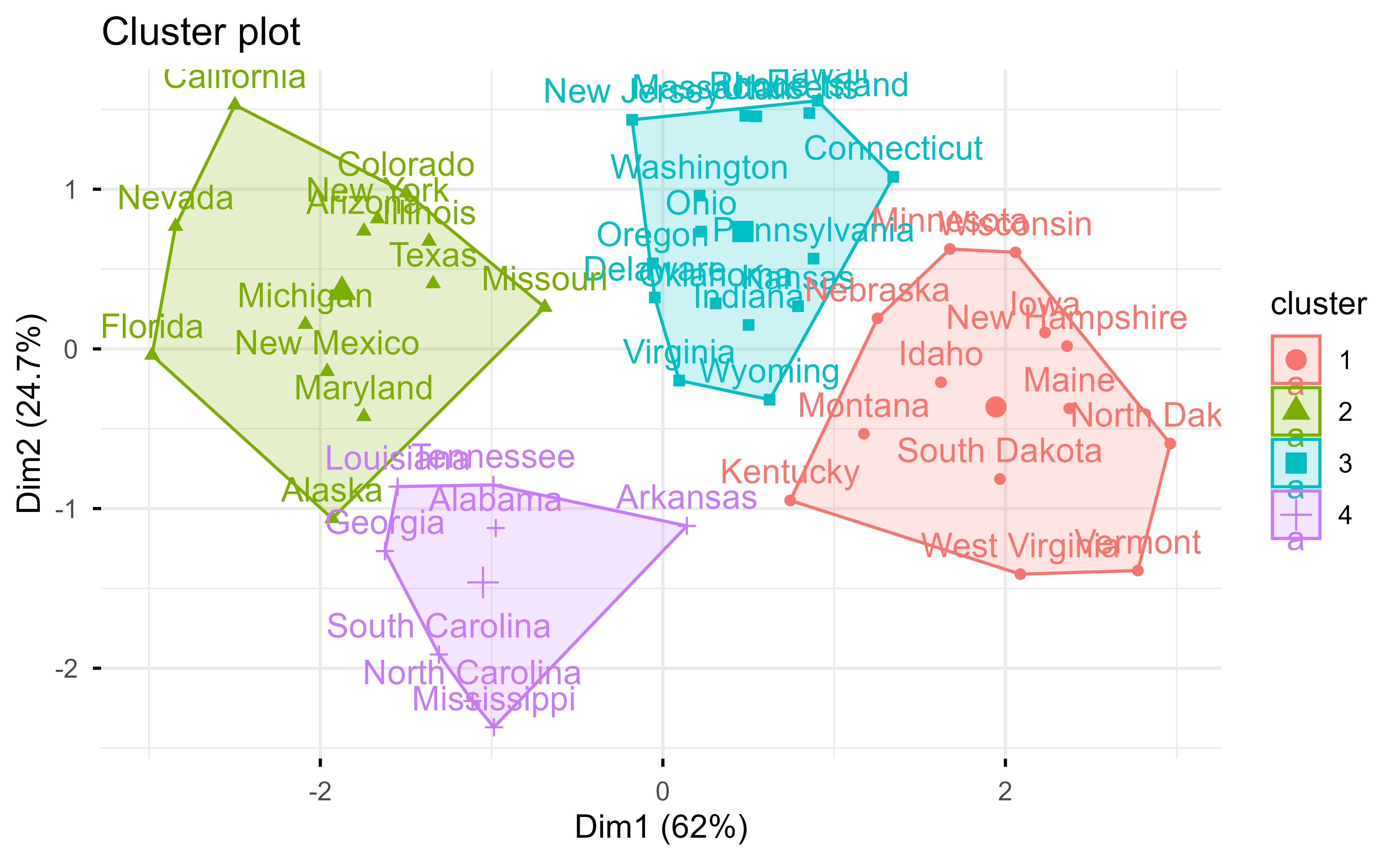
K-means (k = 4, 25 restarts) on standardized USArrests, projected onto the first two principal components.
23.5.3 Choosing k without fooling yourself
Because \(k\) is yours to choose (Section 23.3), lean on more than one diagnostic; they routinely disagree, and the disagreement is information. The elbow and silhouette are quick visual reads (fviz_nbclust(arrests, kmeans, method = "wss") and "silhouette"); the gap statistic compares your within-cluster dispersion against the null of no clustering and is harder to fool:
Show code
set.seed(1)gap<-clusGap(arrests, kmeans, K.max =8, B =50, nstart =25)maxSE(gap$Tab[, "gap"], gap$Tab[, "SE.sim"])# k chosen by the gap statistic#> [1] 3
23.5.4 Hierarchical and medoid variants
Hierarchical clustering avoids committing to \(k\) up front: build the whole tree, then cut. Linkage is the consequential knob — complete (farthest-pair) gives compact clusters, single (nearest-pair) tends to “chain” — so it deserves a deliberate choice, not the default:
Show code
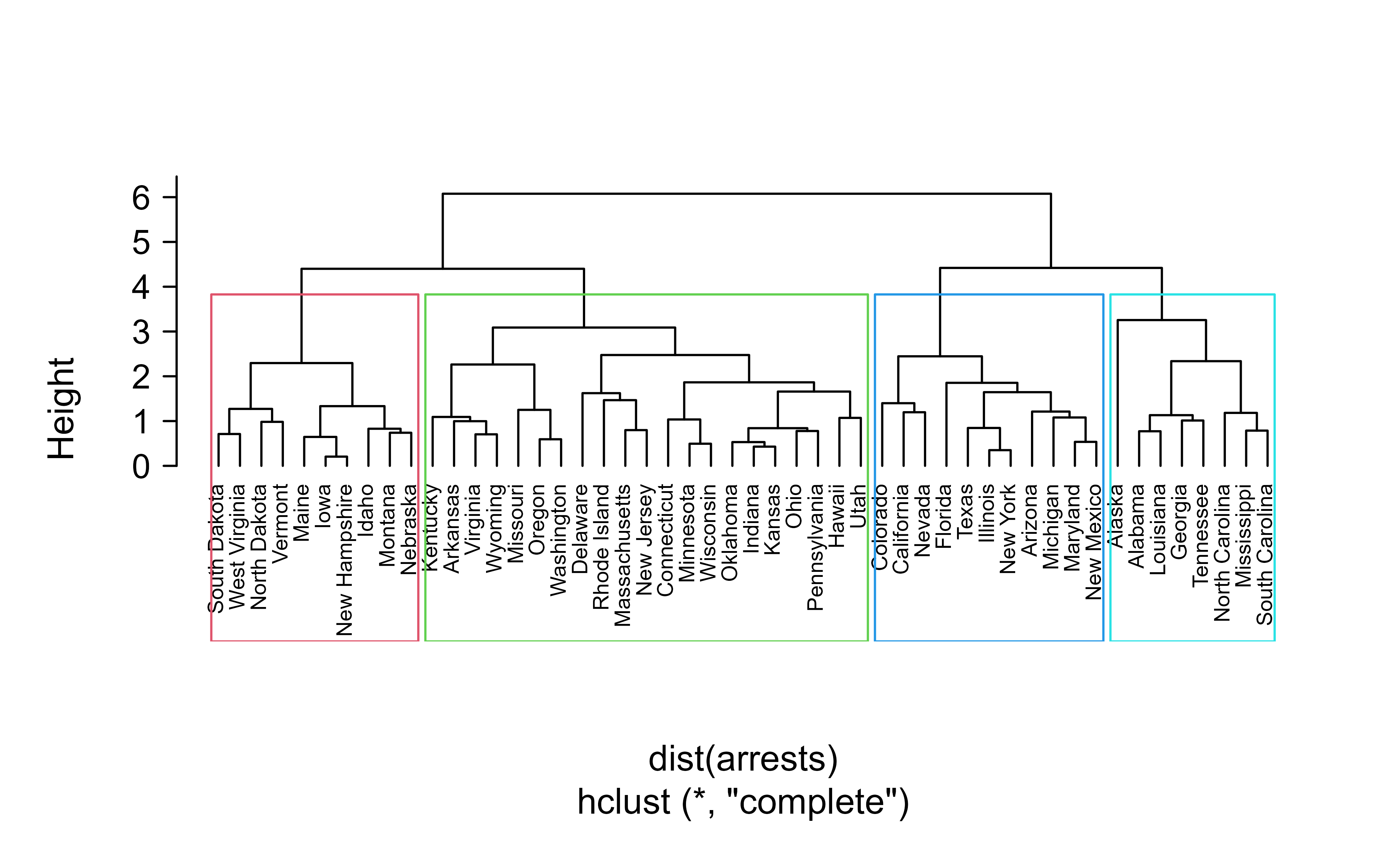
hc<-hclust(dist(arrests), method ="complete")plot(hc, cex =0.6, hang =-1, main ="")rect.hclust(hc, k =4, border =2:5)
Complete-linkage dendrogram of the states, cut into four clusters.
K-medoids (pam) answers a different need: centers that are actual observations (so you can name them) and robustness to outliers, since a medoid cannot be dragged off by one extreme point the way a mean can (Section 23.2.1.3):
Show code
pam(arrests, k =4)$medoids# the representative state for each cluster#> Murder Assault UrbanPop Rape#> Alabama 1.2425641 0.7828393 -0.5209066 -0.003416473#> Michigan 0.9900104 1.0108275 0.5844655 1.480613993#> Oklahoma -0.2727580 -0.2371077 0.1699510 -0.131534211#> New Hampshire -1.3059321 -1.3650491 -0.6590781 -1.252564419
23.5.5 Does the clustering recover real structure?
On USArrests we have no answer key. On iris we do — the species labels — which lets us score a clustering with the adjusted Rand index (chance-corrected agreement; 0 is random, 1 is perfect). We cluster on the four measurements alone, then compare to the held-out species:
An ARI near 0.6 is the honest verdict: K-means cleanly isolates setosa but blurs the versicolor/virginica boundary, because those two species genuinely overlap in feature space. The score keeps us from over-claiming.
23.5.6 When K-means is the wrong tool
Every method so far inherits K-means’ core assumption: clusters are convex blobs around a centroid. Break that assumption and the method breaks with it. Two concentric rings are the textbook counterexample — the “clusters” wrap around a shared center, so no set of centroids can separate them:
Show code
set.seed(1)ring<-function(n, r, s=0.05){th<-seq(0, 2*pi, length.out =n); cbind(r*cos(th)+rnorm(n,0,s), r*sin(th)+rnorm(n,0,s))}rings<-rbind(ring(200, 1), ring(400, 2.5)); truth<-rep(1:2, c(200, 400))km_r<-kmeans(rings, 2, nstart =25)db_r<-dbscan(rings, eps =0.20, minPts =5)# density-based: groups by connectivity, not distance to a centerc(kmeans =adjustedRandIndex(km_r$cluster, truth), dbscan =adjustedRandIndex(db_r$cluster, truth))#> kmeans dbscan #> -0.00144165 1.00000000
K-means scores ~0 (it slices the rings into pie wedges), while DBSCAN scores a perfect 1.0 by following the density of each ring rather than its distance to a center. When your clusters are non-convex, reach for density-based methods like DBSCAN, or for the graph-based spectral clustering of Chapter 25; when you want soft, probabilistic membership instead of hard labels, use the Gaussian mixtures of Section 23.4 via Mclust, which also selects \(k\) and the covariance shape by BIC automatically.
23.5.7 Putting a clustering into production
A subtle gap bites teams in deployment: kmeans returns labels for the training rows but has no predict method for new data. You assign a new observation by standardizing it with the training center and scale (never re-scaling on the new point alone) and snapping it to the nearest centroid:
Show code
predict_kmeans<-function(newdata, km, center, scale){z<-scale(newdata, center =center, scale =scale)apply(z, 1, function(row)which.min(colSums((t(km$centers)-row)^2)))}ctr<-attr(arrests, "scaled:center"); scl<-attr(arrests, "scaled:scale")predict_kmeans(USArrests["California", , drop =FALSE], km, ctr, scl)#> California #> 2
That one function is the difference between a clustering that lives in a notebook and one that can label tomorrow’s records. The broader lesson of this section is that clustering is a sequence of decisions — scale, algorithm, \(k\), linkage, distance — each of which can move the answer, so the defensible workflow validates where it can (ARI when labels exist, gap and silhouette when they do not) and treats the grouping as a hypothesis about structure, never a verdict.
23.6 Summary
Stepping back, clustering is less a single algorithm than a sequence of modeling choices, each of which can move the answer. It is worth gathering those choices and the cautions that go with them in one place.
The dissimilarity measure comes first. Although the standard for hierarchical clustering is Euclidean distance, some applications call for something else. For instance, we might want a correlation-based “distance” that treats two observations as similar when their features move together, even if they sit far apart in Euclidean terms. James et al. (2013) give a useful example of such a measure in a marketing application about shopping preferences, where what matters is the shape of a customer’s buying pattern rather than its overall magnitude.
Several further decisions follow, and most of them do not have a purely objective answer.
You must decide whether to scale the variables to have a standard deviation of one. As with weighting, this depends on the application: scaling prevents a high-variance feature from dominating, but it can also erase a difference that genuinely matters.
If you use Hierarchical Clustering to settle on a certain number of clusters, where you cut the dendrogram is somewhat subjective.
Clustering methods are typically not very robust to perturbations in the data, so small changes to the input can sometimes produce noticeably different groupings. It is wise to check stability rather than trust a single run.
Choosing the number of clusters is always difficult and somewhat subjective, though many methods have been developed to make the choice more objective. The NbClust package, for example, provides 30 indices for determining the relevant number of clusters and reports the best scheme found by varying the number of clusters, the distance measure, and the clustering method.
Finally, everything above treats clustering as a purely geometric, “hard assignment” exercise, but there is another route. We can approach the problem from a model-based, probabilistic perspective by assuming the data are drawn from a mixture of several distributions, often Gaussians though they need not be. Such mixture models are also the basis of model-based density estimation (Chapter 32). The E-M algorithm is an efficient way to estimate such mixtures (Hastie, Friedman, and Tibshirani 2001, 8.5), and as described in (Hastie, Friedman, and Tibshirani 2001, 14.3.7), the mixture-of-Gaussians approach is essentially a “soft” version of K-means, in which each point gets a probability of belonging to each cluster rather than an all-or-nothing label.
Takeaways
Clustering finds the groups implied by your choices, not some objective truth. The choices that matter most are the dissimilarity measure, whether and how you scale or weight features, the algorithm and (for hierarchical methods) the linkage, and the number of clusters. Use multiple random starts for K-means, prefer K-medoids when you need a non-Euclidean dissimilarity or robustness to outliers, read dendrograms from the bottom up and cut them after seeing the structure, and always sanity-check that your clusters survive small perturbations before you trust them.
James, Gareth, Daniela Witten, Trevor Hastie, and Robert Tibshirani. 2013. “Statistical Learning.” In, 15–57. Springer New York. https://doi.org/10.1007/978-1-4614-7138-7_2.
The triangle inequality is the formal statement of “no shortcuts”: going directly from \(i\) to \(i'\) is never longer than detouring through some third point \(k\). Euclidean distance is a metric; some perfectly useful dissimilarities, such as certain correlation-based ones, are only semi-metrics, and that is fine for clustering.↩︎
Manhattan distance measures how far you would travel along a grid of streets, summing the absolute differences coordinate by coordinate, rather than cutting across diagonally as Euclidean distance does. Larger \(\lambda\) puts more emphasis on the single largest coordinate difference.↩︎
The count is given by the Stirling numbers of the second kind, which explode so fast that even a few dozen observations put exhaustive search out of reach.↩︎
An inversion happens when a later merge occurs at a lower height than an earlier one, which breaks the monotonicity that makes a dendrogram readable. Complete and average linkage avoid this and are the usual defaults; single linkage tends to produce stringy, chained clusters.↩︎
Source Code
# Cluster Analysis {#sec-cluster}```{r}#| include: falsesource("_common.R")```Imagine you are handed a spreadsheet of customers, with no labels telling you who is who, and someone asks you to find the "natural groups" hiding inside it. Maybe there is a cluster of frequent, big spenders, another of occasional bargain hunters, and a third of people who signed up once and never returned. Nobody told you these groups exist or what to call them. Your job is to let the data reveal them. That is the goal of cluster analysis: discovering subgroups in a set of features when no answer key is provided.Cluster analysis is a relatively large set of techniques used for finding subgroups, clusters, or segments in a set of features. The guiding idea is simple once you state it plainly. We first decide on some way to measure how similar or dissimilar two observations are, and we then try to form groups that are homogeneous, so that observations *in a subgroup are more similar to each other than to other observations not in the subgroup*. Everything else in this chapter is a way of making that one sentence precise and computable.Because there is no outcome variable telling us the "right" grouping, cluster analysis belongs to unsupervised learning (@sec-intro-unsupervised). This is what separates it from classification methods you may already know. It is worth pausing on that contrast, because both families of methods sort observations into categories, but they do so for different reasons and with different information. @tbl-cluster-vs-discriminant lines up cluster analysis against discriminant analysis, a supervised cousin.|| Cluster Analysis | Discriminant Analysis ||-------------------------------|-----------------------|-----------------------|| Under framework | Unsupervised Learning | Supervised Learning || Dependent variable (category) | No | Yes || Classification rule based on | Closeness | Difference |: Comparison of cluster analysis and discriminant analysis, highlighting that clustering is unsupervised and groups by closeness, while discriminant analysis is supervised and classifies by the differences between known groups. {#tbl-cluster-vs-discriminant}Both discriminant analysis (@sec-discriminant-analysis) and cluster analysis are used to classify, but the resemblance ends there. Discriminant analysis is handed labeled examples and learns rules that exploit the *differences* between known groups; clustering is handed unlabeled data and must invent the groups using nothing but *closeness*.In this chapter you will learn how clustering puts that intuition on a firm footing. We start with how to measure proximity between observations, since every clustering method rests on that choice. We then look at the two best known families of algorithms. K-means clustering partitions observations into a number of clusters you choose in advance. Hierarchical clustering builds a whole tree of nested groupings, so you can decide on the number of clusters after looking at the structure. Along the way we will see the variants K-medoids (a more robust relative of K-means) and the different "linkage" rules that give hierarchical clustering its flavor.A few framing points are worth keeping in mind as we go.- We can cluster the observations to find subgroups of observations, or transpose the problem and cluster the features to find subgroups of features. The machinery is the same; only what plays the role of "object" changes.- Critical to all clustering approaches is the choice of distance, proximity, or dissimilarity measure between two objects. Change that measure and you can change the answer, so we treat it first and treat it carefully.::: {.callout-important title="Key idea"}Clustering does not find the "true" groups in some objective sense. It finds the groups implied by the similarity measure and algorithm you chose. The honest question is never "what are the clusters?" but "what are the clusters *under these assumptions*?":::## Proximity MatricesSince clustering is built entirely on the notion of "alike" versus "different," our first task is to make that notion numerical. It is convenient to represent the data in terms of proximity (alikeness or affinity), which can be expressed either as similarity or as dissimilarity. The distinction is just a matter of direction: a similarity measure increases as two objects become more alike, while a dissimilarity measure decreases as two objects become more alike. Euclidean distance is the familiar example of a dissimilarity measure, since two points sitting on top of each other have distance zero.To use dissimilarity as the foundation for an algorithm, we want it to behave like a sensible notion of distance. Formally, given two $p$-dimensional objects $x_i$ and $x_i'$, a dissimilarity measure $d_{ii'}$ satisfies:1. $d_{ii'} \ge 0 \forall x_i, x_i'$2. $d_{ii'} = 0$ iff $x_i = x_i'$3. $d_{ii'} = d_{i'i}$In words, dissimilarities are never negative, two objects are at distance zero exactly when they are identical, and the dissimilarity from $i$ to $i'$ is the same as from $i'$ to $i$. A measure that satisfies all of these conditions is said to be a semi-metric. If it further satisfies the triangle inequality, $d_{ii'} \le d_{ik} + d_{i'k}$, then it is said to form a metric.^[The triangle inequality is the formal statement of "no shortcuts": going directly from $i$ to $i'$ is never longer than detouring through some third point $k$. Euclidean distance is a metric; some perfectly useful dissimilarities, such as certain correlation-based ones, are only semi-metrics, and that is fine for clustering.]Once we have a dissimilarity measure, we apply it to every pair of observations and collect the results. We typically form the $n \times n$ proximity matrix, $\mathbf{D}$, which in the case of a dissimilarity measure has $(i,j)$th element given by $d_{ij}$. This single matrix is the input that most clustering algorithms actually consume, which is a useful thing to notice: the algorithms never see your raw data directly, only the pairwise dissimilarities you computed from it.::: {.callout-note}Because algorithms operate on $\mathbf{D}$ rather than on the raw features, two completely different datasets that happen to produce the same proximity matrix will be clustered identically. All of your modeling choices about what "similar" means get baked into $\mathbf{D}$ before any clustering begins.:::### Dissimilarities based on AttributesHow do we build the dissimilarity between two whole observations out of their individual features? The usual recipe is to score each attribute separately and then add up the scores. In general, we can define the dissimilarity by summing across the $p$ attributes (that is, with equal weighting):$$d_{ii'} = D(x_i, x_i') = \sum_{j=1}^p d_j (x_{ij}, x_{i'j})$$Here $d_j$ measures dissimilarity on attribute $j$ alone. A very common choice for that per-attribute term is squared distance,$$d_j(x_{ij}, x_{i'j}) = (x_{ij} - x_{i'j})^2$$which, summed over attributes, gives the squared Euclidean distance you already know. This default is reasonable for quantitative variables, but it quietly assumes a lot, and three issues come up in practice.1. We may wish to use more general distance measures.2. We may have categorical variables, which have no natural notion of subtraction.3. We may wish to weight the attributes differently.Each of these has a standard fix.For the first, a general class of dissimilarities is the Minkowski metric,$$d_{ii'} = (\sum_{j=1}^p | x_{ij} - x_{i'j}|^\lambda)^{1/\lambda}$$which contains familiar distances as special cases: $\lambda = 2$ is Euclidean distance, and $\lambda = 1$ is the so-called Manhattan or city-block distance.^[Manhattan distance measures how far you would travel along a grid of streets, summing the absolute differences coordinate by coordinate, rather than cutting across diagonally as Euclidean distance does. Larger $\lambda$ puts more emphasis on the single largest coordinate difference.]The second issue, categorical variables, splits into two cases depending on whether the categories have an order. Consider first the situation where we have ordinal variables (categorical variables that have order, such as "small, medium, large"). Typically one converts these to a numerical value and then uses a quantitative metric. For example, if we have $M$ ordinal values, we can replace them with $(i - 1/2)/M$ for $i = 1, \dots, M$, spreading the categories evenly across the unit interval. For unordered categorical (nominal) variables, there is no order to exploit, so the degree of difference between pairs of values must be specified directly. These values are chosen in a way that maintains the symmetric nature of the dissimilarity matrix.The third issue is weighting, and it is more subtle than it first appears. It is common to weight the elements of the discrepancy function differently depending on the attribute:$$D(x_i, x_i') = \sum_{j=1}^p w_j d_j (x_{ij}, x_{i'j}); \sum_{j=1}^p w_j = 1$$where $w_j$ is a weight assigned to the $j$-th attribute. The natural instinct is that giving every attribute the same weight treats them all "equally," but that instinct is wrong. As discussed in [@hastie2001a 14.3.3], setting the $w_j$ to the same value for each variable does not necessarily give all of the attributes equal *influence*, because a variable that varies over a large range will dominate one that varies over a small range. They show that setting $w_j$ proportional to $1/\bar{d}_j$, where$$\bar{d}_j = \frac{1}{n^2} \sum_{i=1}^n \sum_{i' = 1}^n d_j (x_{ij}, x_{i'j})$$gives all attributes equal influence. The twist is that equal influence is not always what you want, since the attribute that happens to vary the most may be precisely the one that carries the signal about the subgroups.::: {.callout-warning}Standardizing or equalizing the influence of variables is a modeling decision, not a cleanup step. Forcing every feature to contribute equally can wash out the very feature that distinguishes the groups. Decide based on what you know about the problem, not by reflex.:::## Combinatorial Cluster AlgorithmsWe now have a way to measure dissimilarity. The next question is how to turn those dissimilarities into an actual assignment of observations to groups. The cleanest way to state the problem is combinatorial: think of it purely as choosing a label for each observation so as to make groups internally tight.Let each observation be uniquely labeled by an integer $i \in \{1, \dots, n\}$. A pre-specified number of clusters $K<n$ is then assumed, and each cluster is labeled by an integer $k \in \{ 1, \dots, K \}$. Each observation is assigned to one unique cluster. The assignment is characterized by an encoder, $k = C(i)$, which assigns the $i$-th observation to the $k$-th cluster. We seek an encoder based on the dissimilarities $d(x_i, x_i')$ between every pair of observations.To choose among encoders, we have to specify some loss function that we would like the clustering to minimize. A natural one is the within-cluster point scatter,$$W(C) = \frac{1}{2} \sum_{k=1}^K \sum_{C(i)= k} \sum_{C(i') = k} d(x_i, x_{i'})$$which measures the extent to which observations assigned to the same cluster tend to be close to one another. We would like this to be small, since tight clusters are exactly the goal. Its mirror image is the between-cluster point scatter,$$B(C) = \frac{1}{2} \sum_{k=1}^K \sum_{C(i) = k} \sum_{C(i') \neq k} d(x_i, x_{i'})$$which is large when observations assigned to different clusters are far apart, that is, when the clusters are well separated. These two quantities are not independent. Their sum is the total point scatter,$$T = \frac{1}{2} \sum_{i=1}^n \sum_{i'=1}^n d(x_i, x_{i'}) = W(C) + B(C)$$which is constant given the data, independent of the cluster assignment, since it just sums dissimilarity over every pair regardless of labels.This decomposition has a tidy consequence. Because $T$ is fixed, pushing $W(C)$ down automatically pulls $B(C)$ up: minimizing $W(C)$ is equivalent to maximizing $B(C)$. We only ever have to optimize one of them.To see that $T = W(C) + B(C)$ holds for *any* assignment $C$, fix a pair $(i, i')$ and ask which of the two sums it lands in. Every ordered pair appears exactly once in the double sum defining $T$. If $C(i) = C(i')$ the pair contributes to $W(C)$, since the inner sums of $W(C)$ range over pairs in the same cluster; if $C(i) \neq C(i')$ it contributes to $B(C)$. The two cases are mutually exclusive and exhaustive, so summing $W(C)$ and $B(C)$ recovers every pair once, which is exactly $T$. Nothing about this argument used the form of $d$, so the decomposition is purely combinatorial and holds for any dissimilarity.::: {.callout-note title="Why the count is intractable"}The number of distinct ways to partition $n$ objects into exactly $K$ nonempty groups is the Stirling number of the second kind,$$S(n, K) = \frac{1}{K!} \sum_{j=0}^{K} (-1)^j \binom{K}{j} (K-j)^n .$$For fixed $K$ this grows like $K^n / K!$, so the search space is exponential in $n$. Even $S(19, 4) \approx 1.1 \times 10^{10}$, which already rules out enumeration. This is why every practical method below is a greedy or iterative *heuristic* that returns a local optimum, and why K-means clustering (minimizing $W(C)$ for squared Euclidean $d$) is in fact NP-hard in general, both when $K$ is part of the input and even for $K = 2$ in general dimension.:::::: {.callout-tip title="Intuition"}The total amount of "spread" in your data is a fixed budget. Clustering does not reduce that spread; it only decides how much of it sits *inside* groups versus *between* them. Good clusters keep the within-group share small, which is the same as keeping the between-group share large.:::In principle, one could solve this optimization problem exactly by considering every possible combination of observations and cluster assignments, then keeping the best. But the number of ways to partition $n$ points into $K$ groups grows astronomically, so such combinatorial algorithms are computationally prohibitive for most real-world datasets.^[The count is given by the Stirling numbers of the second kind, which explode so fast that even a few dozen observations put exhaustive search out of reach.] In practice we settle for less: iterative descent algorithms that start from some assignment and improve it step by step, converging to a local optimum rather than the global one. The next two sections are exactly such algorithms.### K-Means ClusteringThe K-means algorithm is one of the most popular and useful clustering algorithms, and it is the workhorse you are most likely to reach for first. It is typically used when all the variables are quantitative, and it commits to squared Euclidean distance as the dissimilarity metric:$$d(x_i, x_{i'}) = \sum_{j=1}^p (x_{ij} - x_{i'j})^2 = ||x_i - x_{i'}||^2$$This choice is not arbitrary; it is what lets the algorithm be so simple. With squared Euclidean distance, the within-cluster scatter can be rewritten in a form built around cluster means:$$\begin{aligned}W(C) &= \frac{1}{2} \sum_{k=1}^K \sum_{C(i)=k} \sum_{C(i')=k} ||x_i - x_{i'}||^2 \\&= \sum_{k=1}^K n_k \sum_{C(i)=k} ||x_i - \bar{x}_k||^2\end{aligned}$$where $\bar{x}_k = (\bar{x}_{1k}, \dots, \bar{x}_{pk})$ is the mean vector associated with the $k$-th cluster and $n_k = \sum_{i=1}^n I(C(i)=k)$ is the number of points in cluster $k$. The payoff is the right-hand side: minimizing $W(C)$ amounts to assigning the $n$ observations to the $K$ clusters so that the within-cluster average dissimilarity between each observation and its cluster mean is as small as possible. In other words, the cluster mean (the centroid) is the natural "center" to measure against, and K-means simply alternates between computing centers and reassigning points to the nearest one.#### Deriving the centroid identity {#sec-cluster.qmd-centroid-identity}The collapse from a double sum over pairs to a single sum against the mean is the algebraic heart of K-means, so it is worth doing explicitly. The key is the following identity for any cluster $k$ with $n_k$ members:$$\frac{1}{2} \sum_{C(i)=k} \sum_{C(i')=k} \|x_i - x_{i'}\|^2 = n_k \sum_{C(i)=k} \|x_i - \bar{x}_k\|^2 .$$ {#eq-cluster-pair-to-mean}To prove @eq-cluster-pair-to-mean, expand a single squared pairwise distance by inserting and removing the cluster mean $\bar{x}_k$,$$\|x_i - x_{i'}\|^2 = \|(x_i - \bar{x}_k) - (x_{i'} - \bar{x}_k)\|^2= \|x_i - \bar{x}_k\|^2 + \|x_{i'} - \bar{x}_k\|^2 - 2 (x_i - \bar{x}_k)^\top (x_{i'} - \bar{x}_k) .$$Now sum over all ordered pairs $i, i'$ in cluster $k$. The first term gives $n_k \sum_{C(i)=k} \|x_i - \bar{x}_k\|^2$ because the index $i'$ is free and runs over $n_k$ values; the second term gives the same quantity by symmetry. The cross term vanishes:$$\sum_{C(i)=k} \sum_{C(i')=k} (x_i - \bar{x}_k)^\top (x_{i'} - \bar{x}_k)= \Big( \sum_{C(i)=k} (x_i - \bar{x}_k) \Big)^\top \Big( \sum_{C(i')=k} (x_{i'} - \bar{x}_k) \Big) = 0 ,$$since $\sum_{C(i)=k}(x_i - \bar{x}_k) = \sum_{C(i)=k} x_i - n_k \bar{x}_k = 0$ by the definition of the mean. Collecting terms, $\sum_i \sum_{i'} \|x_i - x_{i'}\|^2 = 2 n_k \sum_i \|x_i - \bar{x}_k\|^2$, which is @eq-cluster-pair-to-mean. Summing over $k$ gives the displayed form of $W(C)$ above.#### Why the mean is optimal, and Lloyd's algorithm {#sec-cluster.qmd-lloyd}A second fact justifies *recomputing the mean* at every iteration. For a fixed set of points $S$, the point $m$ minimizing the sum of squared Euclidean distances is the mean:$$\bar{x}_S = \underset{m \in \mathbb{R}^p}{\operatorname{argmin}} \sum_{x \in S} \|x - m\|^2 .$$ {#eq-cluster-mean-minimizer}This follows by differentiating: $\nabla_m \sum_{x \in S} \|x - m\|^2 = -2 \sum_{x \in S}(x - m) = 0$ gives $m = \frac{1}{|S|}\sum_{x \in S} x$, and the objective is strictly convex in $m$ (Hessian $2|S| I \succ 0$), so this stationary point is the unique global minimizer.Putting @eq-cluster-mean-minimizer together with the obvious fact that, holding the centroids fixed, assigning each point to its nearest centroid minimizes the objective over assignments, exposes K-means as block coordinate descent on the joint objective$$J(C, \{m_k\}) = \sum_{k=1}^K \sum_{C(i)=k} \|x_i - m_k\|^2 .$$ {#eq-cluster-kmeans-objective}Lloyd's algorithm alternates the two exact minimizations: the assignment step minimizes $J$ over $C$ with $\{m_k\}$ fixed, and the update step minimizes $J$ over $\{m_k\}$ with $C$ fixed. Because each step is an exact minimization over one block, $J$ is nonincreasing across iterations:$$J(C^{(t)}, m^{(t)}) \;\ge\; J(C^{(t+1)}, m^{(t)}) \;\ge\; J(C^{(t+1)}, m^{(t+1)}) .$$Since $J \ge 0$ is bounded below and there are only finitely many distinct assignments $C$ (at most $K^n$), the monotone sequence of objective values must stabilize, and the algorithm terminates in a finite number of iterations at a partition that is a local optimum (no single reassignment or recentering lowers $J$). This is exactly the convergence claim made informally above. It is not, however, a global optimum: the result depends on the initialization, which motivates multiple random starts.::: {.callout-warning title="Local optima and a smarter start"}Uniformly random initial assignments can place all seeds in one region and leave genuine clusters merged. The k-means++ seeding rule of Arthur and Vassilvitskii samples the first center uniformly, then samples each subsequent center with probability proportional to its squared distance to the nearest already-chosen center (so far-away points are favored). This spreads seeds out and yields the guarantee $\mathbb{E}[J_{\text{k-means++}}] \le 8(\ln K + 2)\, J_{\text{opt}}$, an $O(\log K)$ approximation in expectation before any Lloyd iterations are even run. In R, `kmeans()` does not implement k-means++ directly, but combining several random starts via `nstart` is the practical substitute, and packages such as `flexclust` offer k-means++ seeding.:::#### Cost, scaling, and failure modes {#sec-cluster.qmd-kmeans-cost}One Lloyd iteration costs $O(nKp)$: each of $n$ points is compared to $K$ centroids in $p$ dimensions, and the centroid update is a single $O(np)$ pass. With $I$ iterations the total is $O(nKpI)$, which is linear in $n$ and is why K-means scales to large datasets where the $O(n^2)$ proximity matrix of the combinatorial view would be prohibitive. The memory footprint is $O(np + Kp)$, since the full $\mathbf{D}$ is never formed.Three failure modes follow directly from the assumptions baked into @eq-cluster-kmeans-objective.- The squared norm makes each cluster an isotropic Gaussian-like ball in the chosen scale, so K-means implicitly assumes clusters of *similar size, similar spread, and roughly spherical shape*. Elongated, curved, or density-varying clusters (two concentric rings, say) are split incorrectly no matter how many restarts you use.- Squared distance squares the influence of outliers, so a single far point can drag a centroid and corrupt an entire cluster. This is the robustness argument for K-medoids.- Because the objective decreases monotonically in $K$ (more centroids can only reduce $J$, reaching $J = 0$ when $K = n$), $J$ alone cannot choose $K$; you need an external criterion (see @sec-cluster.qmd-choosing-k).That alternation is the whole algorithm, given in [@hastie2001a Alg 14.1] and [@james2013 Alg 12.1].1. Randomly assign a number ($1 \to K$) to each of the observations. These are the initial cluster assignments.2. Iterate until the cluster assignments stop changing: 1. For each of the $K$ clusters, compute the cluster centroid. The $k$-th cluster centroid is the vector of the $p$ feature means for the observations in the $k$-th cluster. 2. Assign each observation to the cluster whose centroid is closest, where closest is defined by Euclidean distance.Each pass makes the within-cluster scatter no worse, which is why the procedure is guaranteed to settle down. Two practical points deserve emphasis.- The number of clusters $K$ is yours to choose, and it genuinely matters: ask for three clusters and you get three, whether or not three is meaningful. The algorithm will not warn you that a different $K$ tells a cleaner story.- Although the K-means algorithm is guaranteed to converge, it is not guaranteed to converge to the global minimum. Because it finds a local minimum that depends on the random starting assignment, we should run the algorithm several times from different initial cluster assignments and keep the best result, meaning the one with the smallest value of the objective function $W(C)$.::: {.callout-tip}Always run K-means with multiple random starts and report the best. A single run can land in a poor local optimum that looks fine until you compare it against a few others. Most software exposes this as an `nstart`-style argument; set it to a number like 20 or 50 rather than leaving it at 1.:::### K-Medoids ClusteringK-means is fast and intuitive, but it is wedded to squared Euclidean distance and to using the mean as a cluster center, and the mean is sensitive to outliers and undefined for non-numeric data. K-medoids loosens both restrictions. The key observation is that as long as you can construct a proximity matrix representing the dissimilarity between any two observations, this type of algorithm can be used with any dissimilarity measure you like, not just Euclidean distance. The trick is to insist that each cluster's center be an actual observation (a medoid) rather than an abstract mean.The procedure, from [@hastie2001a, Alg 14.2], mirrors K-means but swaps "mean" for "most central member."1. For a given cluster assignment $C$, find the observation in each cluster that minimizes the total distance to the other points in that cluster:$$i_k^* = \underset{\{ i:C(i) = k\}}{\operatorname{argmin}} \sum_{C(i') = k} D(x_i, x_{i'})$$Then $m_k = x_{i_k^*}, k = 1, 2, \dots, K$ are the current estimates of the cluster centers.2. Given a current set of cluster centers $\{m_1, \dots, m_K\}$, minimize the total error by assigning each observation to the closest current cluster center:$$C(i) = \underset{1 \le k \le K}{\operatorname{argmin}} D(x_i, m_k)$$3. Iterate steps 1 and 2 until the assignments do not change.::: {.callout-tip title="When to use this"}Reach for K-medoids instead of K-means when your dissimilarity is not Euclidean (for example, you only have a precomputed distance matrix), when outliers would distort an arithmetic mean, or when you want each cluster represented by a real, interpretable example rather than an average point. The cost is more computation, since finding the medoid means searching within each cluster.:::The objective being minimized is the total dissimilarity to the assigned medoid,$$J_{\text{med}}(C, \{m_k\}) = \sum_{k=1}^K \sum_{C(i)=k} D(x_i, m_k), \qquad m_k \in \{x_1, \dots, x_n\} ,$$ {#eq-cluster-pam-objective}with the constraint that each center is one of the observations. The same block-descent argument as for K-means applies: step 1 minimizes @eq-cluster-pam-objective over medoids with the assignment fixed, step 2 minimizes over the assignment with medoids fixed, each step is nonincreasing, and the objective is bounded below, so the alternation converges to a local optimum. The exchange between mean and medoid is exactly the difference between minimizing a sum of *squared* Euclidean distances, whose minimizer is the unconstrained mean (@eq-cluster-mean-minimizer), and minimizing a sum of arbitrary dissimilarities over the discrete set of data points.The robustness gain has a cost in complexity. The alternating scheme above costs $O(n_k^2)$ per cluster for the medoid search in step 1, since every candidate medoid is compared against every other member, giving roughly $O(n^2)$ per iteration once summed over clusters. The classical Partitioning Around Medoids (PAM) algorithm of Kaufman and Rousseeuw instead evaluates every candidate swap of a medoid with a non-medoid, costing $O(K(n-K)^2)$ per iteration, which is more thorough but scales poorly. For large $n$ the CLARA variant runs PAM on random subsamples, and the modern FasterPAM algorithm reduces the per-iteration cost by an order of magnitude. In R these are `cluster::pam`, `cluster::clara`, and the `fastkmedoids` package; all consume a precomputed $\mathbf{D}$, which is what lets them work with any dissimilarity.### Hierarchical ClusteringBoth methods so far make you commit to the number of clusters before you see any structure, which is awkward when you genuinely do not know how many groups to expect. Often we would prefer to examine potential clusterings without specifying the number of clusters *a priori*. Hierarchical clustering allows exactly this: instead of one partition, it produces a whole nested sequence of them, from "every point its own cluster" all the way up to "one cluster containing everything," and lets you pick the level afterward.There are two directions you can build this hierarchy.1. Bottom-up (agglomerative): start with each observation as its own cluster, then repeatedly combine the pair of clusters with the smallest intergroup dissimilarity.2. Top-down (divisive): start with one big cluster, then repeatedly split off the group with the largest between-group dissimilarity.We focus on the agglomerative methods, which are by far the more common. A pleasant feature of these methods is that they possess a monotonicity property, so the dissimilarity between merged clusters is monotone increasing with the level of the merge. This is what makes the output interpretable: for any two observations, we look for the point in the tree where the branches containing those two observations are first fused, and the height of that fusion indicates how different the two observations are. The resulting tree plot is called a dendrogram.::: {.callout-tip title="Intuition"}Read a dendrogram from the bottom up. Points that join near the floor are very similar; points whose branches do not merge until near the ceiling are very different. To get $k$ clusters, draw a horizontal line across the tree and count the branches it crosses, then slide the line up or down to get fewer or more clusters. The whole point is that you make that cut *after* seeing the structure, not before.:::The agglomerative procedure itself is short [@james2013, Alg 12.3]:1. Begin with $n$ observations and a measure (for example, Euclidean distance) of all $\binom{n}{2}= n(n-1)/2$ pairwise dissimilarities. Treat each observation as its own cluster.2. For $i = n, n-1, \dots, 2$: 1. Examine all pairwise inter-cluster dissimilarities among the $i$ clusters and identify the pair of clusters that are least dissimilar (most similar). Fuse these two clusters. The dissimilarity between them indicates the height in the dendrogram at which the fusion should be placed. 2. Compute the new pairwise inter-cluster dissimilarities among the $i-1$ remaining clusters.There is one decision hidden in step 2a that we have glossed over. We know how to measure dissimilarity between two single observations, but once clusters contain several points, how do we measure dissimilarity between two *groups*? The agglomerative algorithm requires us to select a rule for this, called linkage, and the choice shapes the kinds of clusters you get. The four most common linkage types are summarized in @tbl-cluster-linkage-types [@james2013, 12.3].| Linkage | Description ||----------|--------------------------------------------------------------------------------------------------------------------------------------------------------------------------------------------------------------------------------------------------------------------------------------------------------------------|| Complete | Maximal intercluster dissimilarity. Compute all pairwise dissimilarities between the observations in cluster A and the observations in cluster B, and record the largest of these dissimilarities || Single | Minimal intercluster dissimilarity. Compute all pairwise dissimilarities between the observations in cluster A and the observations in cluster B, and record the smallest of these dissimilarities. Single linage can result in extended, trailing cluster in which single observation are fused one-at-a-time || Average | Mean intercluster dissimilarity. Compute all pairwise dissimilarities between the observations in cluster A and the observations in cluster B, and record the average fo these dissimilarities || Centroid | Dissimilarity between the centroid for cluster A (a mean vector of length $p$) and the centroid for cluster B. Centroid linkage can result in undesirable *inversions*. |: The four most common linkage rules used to define the dissimilarity between two clusters in agglomerative hierarchical clustering, along with the kinds of cluster shapes each tends to produce. {#tbl-cluster-linkage-types}Different linkage rules can produce genuinely different clusterings from the very same data, so this is not a minor knob.^[An *inversion* happens when a later merge occurs at a lower height than an earlier one, which breaks the monotonicity that makes a dendrogram readable. Complete and average linkage avoid this and are the usual defaults; single linkage tends to produce stringy, chained clusters.] Complete and average linkage tend to yield balanced, compact clusters and are the common defaults, while single linkage can chain observations into long, trailing groups.#### The Lance-Williams update {#sec-cluster.qmd-lance-williams}A naive reading of the algorithm suggests recomputing all inter-cluster dissimilarities from scratch after every merge, but this is unnecessary. When clusters $A$ and $B$ are fused into $A \cup B$, the dissimilarity from the new cluster to any other cluster $C$ can be written as a function of the *old* dissimilarities $d(A,C)$, $d(B,C)$, and $d(A,B)$ alone. This is the Lance-Williams recurrence,$$d(A \cup B, C) = \alpha_A\, d(A,C) + \alpha_B\, d(B,C) + \beta\, d(A,B) + \gamma\, |d(A,C) - d(B,C)| ,$$ {#eq-cluster-lance-williams}where the coefficients select the linkage. Writing $n_A, n_B, n_C$ for cluster sizes, the four rules above correspond to| Linkage | $\alpha_A$ | $\alpha_B$ | $\beta$ | $\gamma$ ||----------|------------|------------|---------|----------|| Single | $1/2$ | $1/2$ | $0$ | $-1/2$ || Complete | $1/2$ | $1/2$ | $0$ | $+1/2$ || Average | $\frac{n_A}{n_A+n_B}$ | $\frac{n_B}{n_A+n_B}$ | $0$ | $0$ || Centroid | $\frac{n_A}{n_A+n_B}$ | $\frac{n_B}{n_A+n_B}$ | $-\frac{n_A n_B}{(n_A+n_B)^2}$ | $0$ |: Lance-Williams coefficients for common linkages (Ward's method is also expressible in this form). {#tbl-cluster-lance-williams}The single and complete cases are immediate: with $\alpha_A = \alpha_B = \tfrac12$ and $\gamma = \mp\tfrac12$, @eq-cluster-lance-williams reduces to $\min\{d(A,C), d(B,C)\}$ and $\max\{d(A,C), d(B,C)\}$ respectively, via the identity $\min(a,b) = \tfrac12(a+b) - \tfrac12|a-b|$ and the matching one for $\max$. The recurrence is what makes agglomerative clustering practical: each of the $n-1$ merges updates a row of the working dissimilarity matrix in $O(n)$ time, giving an $O(n^2)$ time and $O(n^2)$ memory algorithm overall (single linkage can be done in $O(n^2)$ via the minimum spanning tree, and average and complete in $O(n^2 \log n)$ with priority queues). The quadratic memory in $\mathbf{D}$ is the practical ceiling on $n$ for hierarchical methods, in contrast to the linear memory of K-means.The centroid row also explains the inversions warned about in @tbl-cluster-linkage-types: its $\beta < 0$ term can make a fused cluster *closer* to a third cluster than its parts were, so a later merge height can fall below an earlier one. Single, complete, and average linkage have $\beta \ge 0$ and are provably inversion-free (the merge heights are monotone), which is the formal content of the monotonicity property mentioned earlier.## Choosing the Number of Clusters {#sec-cluster.qmd-choosing-k}K-means and K-medoids both require $K$ up front, and the within-cluster objective cannot supply it, since it decreases monotonically toward zero as $K \to n$. Several principled criteria fill the gap.The simplest is the elbow heuristic: plot $W_K$, the total within-cluster scatter at the optimum for each $K$, against $K$ and look for the value where the marginal decrease flattens. The reasoning is that adding a center inside a true cluster yields little reduction, whereas splitting two genuine clusters yields a large one, so the curve bends at the true number. The elbow is often ambiguous, which motivates sharper tools.The gap statistic of Tibshirani, Walther, and Hastie formalizes the elbow by comparing $\log W_K$ to its expectation under a null reference distribution with no clustering (typically uniform over the data's bounding box or its principal-component box):$$\text{Gap}(K) = \mathbb{E}^*_n[\log W_K] - \log W_K ,$$ {#eq-cluster-gap}where $\mathbb{E}^*_n$ is estimated by clustering $B$ Monte Carlo reference samples. One chooses the smallest $K$ such that $\text{Gap}(K) \ge \text{Gap}(K+1) - s_{K+1}$, where $s_{K+1}$ is the standard error of the reference $\log W$ values inflated by $\sqrt{1 + 1/B}$. A key virtue is that the gap statistic can return $K = 1$, that is, no clustering structure, which the elbow and silhouette cannot.The silhouette of Rousseeuw scores each point $i$ individually. Let $a(i)$ be its mean dissimilarity to other points in its own cluster, and $b(i)$ the mean dissimilarity to the points of the nearest *other* cluster. The silhouette width is$$s(i) = \frac{b(i) - a(i)}{\max\{a(i),\, b(i)\}} \in [-1, 1] ,$$ {#eq-cluster-silhouette}which is near $+1$ when $i$ sits comfortably inside its cluster and far from the next, near $0$ on a boundary, and negative when $i$ is probably misassigned. Averaging $s(i)$ over all points gives a single number, and the $K$ maximizing the average silhouette is selected. Because it uses only pairwise dissimilarities, the silhouette applies equally to K-medoids and to any non-Euclidean $\mathbf{D}$. In R, `cluster::silhouette`, `factoextra::fviz_nbclust`, and the 30-index `NbClust` package automate these comparisons.::: {.callout-warning}None of these indices is a hypothesis test with a guaranteed error rate, and they routinely disagree. Treat $K$ selection as exploratory: cross-check at least two criteria, confirm the chosen clusters are stable under resampling, and prefer a $K$ that is also interpretable in the application over one that wins a single index by a hair.:::## Model-Based Clustering and the K-Means Connection {#sec-cluster.qmd-gmm}The geometric view treats clustering as minimizing a distance objective. The model-based view instead posits a generative probability model and clusters by fitting it, which has the advantage of supplying soft memberships, a principled likelihood for comparing $K$, and the ability to capture clusters that are not spherical. The canonical model is the Gaussian mixture,$$p(x) = \sum_{k=1}^K \pi_k\, \mathcal{N}(x \mid \mu_k, \Sigma_k), \qquad \pi_k \ge 0, \ \sum_k \pi_k = 1 ,$$ {#eq-cluster-gmm-density}where $\pi_k$ is the prior weight of component $k$. Introducing a latent indicator $z_i \in \{1,\dots,K\}$ with $P(z_i = k) = \pi_k$ and $x_i \mid z_i = k \sim \mathcal{N}(\mu_k, \Sigma_k)$ makes the log-likelihood tractable through the EM algorithm.The **E-step** computes the posterior responsibility of component $k$ for point $i$ via Bayes' rule:$$\gamma_{ik} = P(z_i = k \mid x_i) = \frac{\pi_k\, \mathcal{N}(x_i \mid \mu_k, \Sigma_k)}{\sum_{l=1}^K \pi_l\, \mathcal{N}(x_i \mid \mu_l, \Sigma_l)} .$$ {#eq-cluster-estep}The **M-step** maximizes the expected complete-data log-likelihood, yielding responsibility-weighted moment estimates:$$\pi_k = \frac{1}{n}\sum_{i=1}^n \gamma_{ik}, \qquad\mu_k = \frac{\sum_i \gamma_{ik}\, x_i}{\sum_i \gamma_{ik}}, \qquad\Sigma_k = \frac{\sum_i \gamma_{ik}\,(x_i - \mu_k)(x_i - \mu_k)^\top}{\sum_i \gamma_{ik}} .$$ {#eq-cluster-mstep}EM increases the observed-data log-likelihood at every iteration and converges to a local maximum, exactly paralleling Lloyd's monotone descent.K-means is the hard-assignment, equal-isotropic-covariance limit of this procedure. Fix $\Sigma_k = \sigma^2 I$ and $\pi_k = 1/K$ for all $k$, and let $\sigma^2 \to 0$. The Gaussian density is $\mathcal{N}(x_i \mid \mu_k, \sigma^2 I) \propto \exp(-\|x_i - \mu_k\|^2 / 2\sigma^2)$, so the responsibility in @eq-cluster-estep becomes$$\gamma_{ik} = \frac{\exp(-\|x_i - \mu_k\|^2 / 2\sigma^2)}{\sum_l \exp(-\|x_i - \mu_l\|^2 / 2\sigma^2)} .$$As $\sigma^2 \to 0$ this softmax sharpens to an indicator: the term with the smallest $\|x_i - \mu_k\|^2$ dominates, so $\gamma_{ik} \to 1$ for the nearest center and $0$ otherwise. That is precisely the K-means assignment step, and the M-step update for $\mu_k$ in @eq-cluster-mstep collapses to the cluster mean, which is the K-means update step. Thus K-means is "hard EM" for a spherical, equal-weight Gaussian mixture in the zero-variance limit, the formal version of the statement that the mixture model is a soft version of K-means. Relaxing the fixed isotropic $\Sigma_k$ is what lets GMMs model elliptical and differently-sized clusters that defeat K-means; in R this is `mclust`, which additionally selects $K$ and the covariance structure by BIC. The price is more parameters ($O(K p^2)$ for full covariances) and the same sensitivity to initialization and to degenerate likelihood spikes when a component collapses onto a single point.::: {.callout-note title="Verification: K-means as the hard-EM limit"}The simulation below fits a one-dimensional, two-component spherical GMM by EM with the variance pinned at a small value, and checks that the resulting hard assignments and centers match `kmeans`.```{r}#| label: kmeans-em-limit#| eval: falseset.seed(1)x <-c(rnorm(200, -3), rnorm(200, 3)) # two well-separated groupssig2 <-1e-3# tiny fixed variancemu <-c(-1, 1) # initial centersfor (it in1:50) { d <-outer(x, mu, function(a, b) (a - b)^2) # squared distances g <-exp(-d / (2* sig2)) g <- g /rowSums(g) # responsibilities (E-step) mu <-colSums(g * x) /colSums(g) # weighted means (M-step)}em_centers <-sort(mu)km_centers <-sort(kmeans(x, centers =2, nstart =10)$centers[, 1])rbind(em = em_centers, kmeans = km_centers) # should match closely```:::## Clustering in R: A Worked Example {#sec-cluster-worked}The theory above makes several claims that are easy to state and easy to forget: that scale silently decides the answer, that K-means only finds a local optimum, that "the number of clusters" is a modeling choice rather than a fact, and that the whole enterprise assumes clusters are roughly convex blobs. Rather than restate them, this section makes each one *happen* in code, on data small enough to audit. We lean on `cluster`, `factoextra` (for cluster plots), `mclust` (model-based clustering and the adjusted Rand index), and `dbscan`.```{r}#| label: cluster-setuplibrary(cluster); library(factoextra); library(mclust); library(dbscan)```### Scale is a modeling decision, not a formality`USArrests` records four crime statistics for the 50 US states. Look at their spreads before doing anything else:```{r}#| label: cluster-scalesround(sapply(USArrests, sd), 1)````Assault` has a standard deviation near 83 while `Murder`'s is around 4. Euclidean distance squares those differences, so on the raw data `Assault` contributes roughly $(83/4)^2 \approx 430$ times the influence of `Murder` --- the clustering would essentially be "sort states by assault rate." Standardizing puts every feature on equal footing, which is the right default unless you have a substantive reason to privilege one (@sec-cluster.qmd-kmeans-cost):```{r}#| label: cluster-standardizearrests <-scale(USArrests) # mean 0, sd 1 per column```### K-means and the local-optimum trapLloyd's algorithm (@sec-cluster.qmd-lloyd) descends to a *local* minimum that depends on where the centers start. This is not a footnote --- it changes answers. Run it twenty times from a single random start each and watch the within-cluster sum of squares wander:```{r}#| label: cluster-localoptimaspread <-sapply(1:20, function(s) { set.seed(s); kmeans(arrests, 4, nstart =1)$tot.withinss })range(spread) # best vs worst local optimum from one random start```The fix is not cleverness but repetition: `nstart` runs many initializations and keeps the best. This is why you should essentially never call `kmeans` with the default `nstart = 1` in production.```{r}#| label: cluster-kmeans#| fig-cap: "K-means (k = 4, 25 restarts) on standardized USArrests, projected onto the first two principal components."set.seed(1)km <-kmeans(arrests, centers =4, nstart =25)km$sizefviz_cluster(km, data = arrests, ggtheme =theme_minimal())```### Choosing k without fooling yourselfBecause $k$ is yours to choose (@sec-cluster.qmd-choosing-k), lean on more than one diagnostic; they routinely disagree, and the disagreement is information. The elbow and silhouette are quick visual reads (`fviz_nbclust(arrests, kmeans, method = "wss")` and `"silhouette"`); the **gap statistic** compares your within-cluster dispersion against the null of no clustering and is harder to fool:```{r}#| label: cluster-gapset.seed(1)gap <-clusGap(arrests, kmeans, K.max =8, B =50, nstart =25)maxSE(gap$Tab[, "gap"], gap$Tab[, "SE.sim"]) # k chosen by the gap statistic```### Hierarchical and medoid variantsHierarchical clustering avoids committing to $k$ up front: build the whole tree, then cut. Linkage is the consequential knob --- `complete` (farthest-pair) gives compact clusters, `single` (nearest-pair) tends to "chain" --- so it deserves a deliberate choice, not the default:```{r}#| label: cluster-hclust#| fig-cap: "Complete-linkage dendrogram of the states, cut into four clusters."hc <-hclust(dist(arrests), method ="complete")plot(hc, cex =0.6, hang =-1, main ="")rect.hclust(hc, k =4, border =2:5)```K-medoids (`pam`) answers a different need: centers that are *actual observations* (so you can name them) and robustness to outliers, since a medoid cannot be dragged off by one extreme point the way a mean can (@sec-cluster.qmd-kmeans-cost):```{r}#| label: cluster-pampam(arrests, k =4)$medoids # the representative state for each cluster```### Does the clustering recover real structure?On `USArrests` we have no answer key. On `iris` we do --- the species labels --- which lets us *score* a clustering with the **adjusted Rand index** (chance-corrected agreement; 0 is random, 1 is perfect). We cluster on the four measurements alone, then compare to the held-out species:```{r}#| label: cluster-ariX <-scale(iris[, 1:4]); set.seed(1)km_iris <-kmeans(X, centers =3, nstart =25)adjustedRandIndex(km_iris$cluster, iris$Species)```An ARI near 0.6 is the honest verdict: K-means cleanly isolates *setosa* but blurs the *versicolor*/*virginica* boundary, because those two species genuinely overlap in feature space. The score keeps us from over-claiming.### When K-means is the wrong toolEvery method so far inherits K-means' core assumption: clusters are convex blobs around a centroid. Break that assumption and the method breaks with it. Two concentric rings are the textbook counterexample --- the "clusters" wrap around a shared center, so no set of centroids can separate them:```{r}#| label: cluster-rings#| fig-cap: "Two concentric rings: K-means (left) splits them by angle; DBSCAN (right) recovers them exactly."set.seed(1)ring <-function(n, r, s =0.05) { th <-seq(0, 2*pi, length.out = n); cbind(r*cos(th) +rnorm(n,0,s), r*sin(th) +rnorm(n,0,s)) }rings <-rbind(ring(200, 1), ring(400, 2.5)); truth <-rep(1:2, c(200, 400))km_r <-kmeans(rings, 2, nstart =25)db_r <-dbscan(rings, eps =0.20, minPts =5) # density-based: groups by connectivity, not distance to a centerc(kmeans =adjustedRandIndex(km_r$cluster, truth),dbscan =adjustedRandIndex(db_r$cluster, truth))```K-means scores ~0 (it slices the rings into pie wedges), while DBSCAN scores a perfect 1.0 by following the *density* of each ring rather than its distance to a center. When your clusters are non-convex, reach for density-based methods like DBSCAN, or for the graph-based spectral clustering of @sec-spectral-clustering; when you want soft, probabilistic membership instead of hard labels, use the Gaussian mixtures of @sec-cluster.qmd-gmm via `Mclust`, which also selects $k$ and the covariance shape by BIC automatically.### Putting a clustering into productionA subtle gap bites teams in deployment: `kmeans` returns labels for the *training* rows but has no `predict` method for new data. You assign a new observation by standardizing it with the *training* center and scale (never re-scaling on the new point alone) and snapping it to the nearest centroid:```{r}#| label: cluster-predictpredict_kmeans <-function(newdata, km, center, scale) { z <-scale(newdata, center = center, scale = scale)apply(z, 1, function(row) which.min(colSums((t(km$centers) - row)^2)))}ctr <-attr(arrests, "scaled:center"); scl <-attr(arrests, "scaled:scale")predict_kmeans(USArrests["California", , drop =FALSE], km, ctr, scl)```That one function is the difference between a clustering that lives in a notebook and one that can label tomorrow's records. The broader lesson of this section is that clustering is a sequence of decisions --- scale, algorithm, $k$, linkage, distance --- each of which can move the answer, so the defensible workflow validates where it can (ARI when labels exist, gap and silhouette when they do not) and treats the grouping as a hypothesis about structure, never a verdict.## SummaryStepping back, clustering is less a single algorithm than a sequence of modeling choices, each of which can move the answer. It is worth gathering those choices and the cautions that go with them in one place.The dissimilarity measure comes first. Although the standard for hierarchical clustering is Euclidean distance, some applications call for something else. For instance, we might want a correlation-based "distance" that treats two observations as similar when their features move together, even if they sit far apart in Euclidean terms. @james2013 give a useful example of such a measure in a marketing application about shopping preferences, where what matters is the *shape* of a customer's buying pattern rather than its overall magnitude.Several further decisions follow, and most of them do not have a purely objective answer.- You must decide whether to scale the variables to have a standard deviation of one. As with weighting, this depends on the application: scaling prevents a high-variance feature from dominating, but it can also erase a difference that genuinely matters.- If you use [Hierarchical Clustering] to settle on a certain number of clusters, where you cut the dendrogram is somewhat subjective.- Clustering methods are typically not very robust to perturbations in the data, so small changes to the input can sometimes produce noticeably different groupings. It is wise to check stability rather than trust a single run.- Choosing the number of clusters is always difficult and somewhat subjective, though many methods have been developed to make the choice more objective. The `NbClust` package, for example, provides 30 indices for determining the relevant number of clusters and reports the best scheme found by varying the number of clusters, the distance measure, and the clustering method.Finally, everything above treats clustering as a purely geometric, "hard assignment" exercise, but there is another route. We can approach the problem from a model-based, probabilistic perspective by assuming the data are drawn from a mixture of several distributions, often Gaussians though they need not be. Such mixture models are also the basis of model-based density estimation (@sec-density-estimation). The E-M algorithm is an efficient way to estimate such mixtures [@hastie2001a, 8.5], and as described in [@hastie2001a, 14.3.7], the mixture-of-Gaussians approach is essentially a "soft" version of K-means, in which each point gets a probability of belonging to each cluster rather than an all-or-nothing label.::: {.callout-important title="Takeaways"}Clustering finds the groups implied by your choices, not some objective truth. The choices that matter most are the dissimilarity measure, whether and how you scale or weight features, the algorithm and (for hierarchical methods) the linkage, and the number of clusters. Use multiple random starts for K-means, prefer K-medoids when you need a non-Euclidean dissimilarity or robustness to outliers, read dendrograms from the bottom up and cut them after seeing the structure, and always sanity-check that your clusters survive small perturbations before you trust them.:::