Advanced Data Analysis

Nguyen, Mike

9 Multivariate Adaptive Regression Splines

Imagine you want to predict a house price from dozens of features (square footage, lot size, year built, neighborhood, and so on), and you suspect the relationship is not a straight line. Square footage might matter a lot up to a point and then flatten out; the effect of one feature might depend on the value of another. Plain linear regression cannot capture these bends and interactions on its own, and fitting a separate smooth curve to each predictor by hand quickly becomes unmanageable when there are many inputs.

Multivariate Adaptive Regression Splines (MARS) is a method that handles exactly this situation automatically. It builds a regression model out of simple “hinge” pieces, lines that bend at chosen locations, and it decides on its own where to put the bends, which predictors to use, and which predictors should interact. In this sense MARS sits between two ideas you have already met: it generalizes stepwise linear regression by letting the model add bent (not just straight) terms, and it can be seen as a modification of the CART procedure from the classification and regression trees chapter (Chapter 8) that performs better in the regression setting.¹

By the end of this chapter you will understand the building blocks MARS uses (piecewise linear basis functions, called hinge functions), how the forward, then backward, model-building strategy works, and how the method chooses a final model size. You will also see a short worked example. The core machinery is an expansion in the piecewise linear basis function family.

Note

MARS is not used as much today as it once was, having been largely overtaken by tree ensembles such as gradient boosting (Chapter 12). It remains worth studying because its ideas, adaptive knot selection and automatic interaction discovery, are clear and instructive, and the model it produces is unusually easy to interpret.

How MARS relates to CART

It helps to anchor MARS against CART, since the two share a common spirit but differ in their building blocks. CART splits the feature space with step functions and produces a binary tree; MARS replaces those hard steps with gentle bends and allows more flexible structure. To see the connection, picture starting from a tree-style procedure and making the following changes:

Replace the piecewise linear basis function with step functions (for example, $I(x-t>0)$ and $I(x-t) \le 0$).
When a model term is multiplied by a candidate term, it gets replaced by the resulting interaction and is therefore no longer available for further interaction.

With those two changes, the MARS forward procedure becomes essentially the CART tree-growing algorithm. Multiplying a step function by a pair of reflected step functions is equivalent to splitting a node at that step, and the second restriction (a node may not be split more than once) is what forces the binary tree structure. MARS is more flexible precisely because it drops these restrictions: it keeps smooth hinge functions instead of hard steps, and it allows additive structures rather than being confined to a binary tree.

Key idea

CART is a special, restricted case of the MARS-style construction. Loosening the restrictions (smooth hinges, reusable terms) is what gives MARS its extra power and its ability to represent additive effects.

The building blocks: hinge functions

The atom of a MARS model is a one-sided linear piece. Consider a basis function of the following form, where the “+” subscript means “positive part” with a knot at $t$:

\[ (x-t)_+ = \begin{cases} x-t & \text{ if } x > t \\ 0 & \text{otherwise} \end{cases} \]

and its mirror image,

\[ (t-x)_+ = \begin{cases} t- x & \text{ if } x < t \\ 0 & \text{otherwise} \end{cases} \]

Each of these is flat (equal to zero) on one side of the knot $t$ and rises linearly on the other side. They are linear splines, and because one is the mirror image of the other across $t$, the pair is called a reflected pair.

Intuition

A single hinge function is a “ramp” that switches on at $t$. A reflected pair gives you one ramp going up to the right of $t$ and one going up to the left of $t$. Adding both to a model lets the fitted curve bend at $t$ and take a different slope on each side, which is how MARS turns straight lines into flexible, piecewise-linear shapes.

Where do we put the knots? MARS forms such a reflected pair for each input $X_j$ with knots placed at every observed value $x_{ij}$ of that input. This is what makes the knot placement adaptive: instead of guessing knot locations in advance, the method considers every data point as a candidate. The full collection of basis functions is

\[ C = \{(X_j - t)_+ , (t-X_j)_+\}_{t \in \{x_{1j}, \dots, x_{nj} \}}, j = 1, \dots, p \]

If all input values are distinct, this collection can contain as many as $2np$ basis functions, which can be very large.

The model and how it is built

A MARS model has the form

\[ f(X) = \beta_0 + \sum_{m=1}^M \beta_m h_m (X) \]

where each $h_m(X)$ is either a function drawn from the collection $C$ or a product of two or more such functions. Products are what create interactions between variables. As in forward stepwise linear regression, we build the final model from these transformed inputs rather than from the original inputs directly.

Once the set of terms $h_m$ is fixed, estimating the coefficients $\beta_m$ is the easy part: we use ordinary least squares, minimizing the residual sum of squares. The hard and important part is choosing which $h_m(X)$ to include, and that is where the adaptive search comes in.

Formulation: the regression problem MARS solves

Fix the structure of the model, that is, the list of terms $h_0 \equiv 1, h_1, \dots, h_M$. Collect them into the $n \times (M+1)$ design matrix $\mathbf{B}$ with entries $B_{im} = h_m(x_i)$, so column $0$ is a column of ones. Stacking the responses into $\mathbf{y} \in \mathbb{R}^n$ and the coefficients into $\boldsymbol\beta = (\beta_0, \beta_1, \dots, \beta_M)^\top$, MARS solves the ordinary least squares problem

\[ \hat{\boldsymbol\beta} = \arg\min_{\boldsymbol\beta} \; \big\| \mathbf{y} - \mathbf{B}\boldsymbol\beta \big\|_2^2 = (\mathbf{B}^\top \mathbf{B})^{-1} \mathbf{B}^\top \mathbf{y}, \tag{9.1}\]

with fitted values $\hat{\mathbf{y}} = \mathbf{B}\hat{\boldsymbol\beta} = \mathbf{H}\mathbf{y}$ and hat matrix $\mathbf{H} = \mathbf{B}(\mathbf{B}^\top \mathbf{B})^{-1}\mathbf{B}^\top$. The statistical model behind Equation 9.1 is the usual one, $y_i = f(x_i) + \varepsilon_i$ with $\mathbb{E}[\varepsilon_i] = 0$ and $\mathrm{Var}(\varepsilon_i) = \sigma^2$, and $f$ assumed to lie (approximately) in the span of products of hinge functions. The space of functions reachable by MARS is the linear span of the constant together with all products $\prod_{k} (\pm(X_{j_k} - t_k))_+$ that respect two structural constraints stated later: each variable appears at most once in a product, and (by convention) lower-order parts of any product are also present. Within that span the fit is linear in $\boldsymbol\beta$, so for a fixed structure everything reduces to least squares; the difficulty, and all of the adaptivity, is in choosing the structure.

The forward pass: adding terms greedily

We start as simply as possible. The model begins with the constant function $h_0(X) = 1$, and every function in $C$ is a candidate to be added next.

At each stage, we consider every product of a function $h_l$ already in the current model set $M$ with one of the reflected pairs in $C$, that is, terms of the form

\[ \hat{\beta}_{M + 1} h_l(X) \times (X_j -t)_+ + \hat{\beta}_{M + 2} h_l(X) \times (t - X_j )_+, h_l \in M \]

where $h_l$ is some basis function already in the model. Among all such candidate additions, we pick the one that produces the largest decrease in training error, and we add that reflected pair of products to the model set $M$.

Note

Because each new term is a product of an existing term with a new reflected pair, the search naturally discovers interactions. Multiplying by the constant $h_0(X) = 1$ keeps the new term as a simple main effect; multiplying by an existing hinge creates a two-way (or higher) interaction.

To make this concrete, here is how the first couple of stages play out.

First, we consider adding a function of the form $\beta_1 (X_j - t)_+ + \beta_2(t-X_j)_+, t \in \{ x_{ij} \}$ (multiplying by the constant function just produces the reflected pair itself). Suppose that for a particular data set the best choice turns out to be $\hat{\beta}_1 (X_2 - x_{72})_+ + \hat{\beta}_2 (x_{72} - X_2)_+$. We add this to the set $M$.

Next, we consider adding a pair of products of the form

\[ h_m (X) \times (X_j - t)_+ \]

\[ h_m(X) \times (t- X_j)_+, t \in \{ x_{ij} \} \]

where for $h_m$ we now have three choices:

\[ h_0(X) = 1, h_1(X) = (X_2 - x_{72})_+ \]

\[ h_2(X) = (x_{72} - X_2)_+ \]

For example, the third choice can produce an interaction term such as $(X_1 - x_{51})_+ \times (x_{72} - X_2)_+$.

The forward pass continues until a pre-specified number of terms is in the model. By design this gives a large model that overfits the data, which is exactly what we want before pruning.

Derivation: the gain from adding a reflected pair

It is worth seeing exactly what quantity the forward pass maximizes, because it explains why the search is only $O(n)$ per variable and why knots can be tested incrementally. Suppose the current model has design matrix $\mathbf{B}$ and projects $\mathbf{y}$ onto $\mathrm{col}(\mathbf{B})$, leaving residual $\mathbf{r} = \mathbf{y} - \mathbf{B}\hat{\boldsymbol\beta} = (\mathbf{I} - \mathbf{H})\mathbf{y}$. We consider adding the two new columns $\mathbf{u}(t) = h_l \odot (X_j - t)_+$ and $\mathbf{v}(t) = h_l \odot (t - X_j)_+$ (elementwise products evaluated at the data, for a fixed parent $h_l$, variable $j$, and knot $t$). The decrease in residual sum of squares from appending columns $\mathbf{Z} = [\mathbf{u}(t), \mathbf{v}(t)]$ to a model that already contains $\mathbf{B}$ is, by the standard formula for the extra sum of squares of a projection onto the orthogonal complement,

\[ \Delta \mathrm{RSS}(j,t,l) = \tilde{\mathbf{Z}}^\top \mathbf{r} \,\big( \tilde{\mathbf{Z}}^\top \tilde{\mathbf{Z}} \big)^{-1} \tilde{\mathbf{Z}}^\top \mathbf{r}, \qquad \tilde{\mathbf{Z}} = (\mathbf{I} - \mathbf{H})\mathbf{Z}, \tag{9.2}\]

where $\tilde{\mathbf{Z}}$ is $\mathbf{Z}$ orthogonalized against the existing columns. To see Equation 9.2, write the augmented projection in block form: regressing $\mathbf{y}$ on $[\mathbf{B}, \mathbf{Z}]$ is equivalent, by the Frisch to Waugh to Lovell theorem, to first removing $\mathbf{B}$ from both $\mathbf{y}$ and $\mathbf{Z}$ and then regressing the residual $\mathbf{r}$ on $\tilde{\mathbf{Z}}$. The reduction in RSS achieved by that second regression is the squared length of the projection of $\mathbf{r}$ onto $\mathrm{col}(\tilde{\mathbf{Z}})$, namely $\mathbf{r}^\top \tilde{\mathbf{Z}} (\tilde{\mathbf{Z}}^\top \tilde{\mathbf{Z}})^{-1} \tilde{\mathbf{Z}}^\top \mathbf{r}$, which is Equation 9.2. The forward pass selects the triple $(j,t,l)$ maximizing this gain, which is the same as choosing the candidate that minimizes the new training RSS, since the old RSS is fixed.

Two facts make this cheap. First, only $\mathbf{r}$ enters, so the parent fit is computed once per stage. Second, as the knot $t$ sweeps through the sorted values $x_{(1)j} > x_{(2)j} > \dots$ of variable $j$, the column $(X_j - t)_+$ changes by a simple, incremental amount: lowering the knot past one data point adds a constant slope contribution over the points already to the right of $t$. The inner products $\tilde{\mathbf{Z}}^\top \mathbf{r}$ and the small Gram matrix $\tilde{\mathbf{Z}}^\top \tilde{\mathbf{Z}}$ can therefore be updated in $O(1)$ per knot using running sums, giving $O(n)$ work to scan all knots of one variable rather than the naive $O(n^2)$. This is the precise sense of the locality and efficiency claims made later.

Intuition

The strategy is deliberately “grow too big, then trim.” Greedily adding terms is fast but tends to keep some terms that only help on the training set. Pruning afterward removes them.

The backward pass: pruning

To undo the overfitting, MARS uses backward deletion. At each step it removes the single term whose removal causes the smallest increase in residual squared error. Running this all the way down produces, for each model size $\lambda$ (the number of terms), an estimated “best” model $\hat{f}_\lambda$ of that size.

The cost of deleting a term mirrors Equation 9.2. If $\mathbf{B}$ is the current design and we drop column $m$, leaving $\mathbf{B}_{-m}$, the increase in RSS equals the squared length of the part of $\hat{\mathbf{y}}$ that $\mathbf{B}_{-m}$ cannot recover. Writing $\hat\beta_m$ for the fitted coefficient of column $m$ and $\mathbf{w}_m = (\mathbf{I} - \mathbf{H}_{-m})\mathbf{b}_m$ for column $m$ orthogonalized against the others (where $\mathbf{b}_m$ is the $m$th column and $\mathbf{H}_{-m}$ the hat matrix of $\mathbf{B}_{-m}$),

\[ \Delta \mathrm{RSS}_{\text{drop } m} = \hat\beta_m^2 \, \|\mathbf{w}_m\|_2^2 . \tag{9.3}\]

Backward deletion removes, at each step, the surviving term with the smallest value of Equation 9.3 (the constant $h_0$ is never removed). The asymmetry with the forward pass is deliberate: the forward pass must add reflected pairs to keep the candidate set rich, but backward deletion removes terms one at a time, so it can keep a useful “up” hinge while discarding its unused mirror image.

Choosing the model size

We are left with a sequence of candidate models of different sizes and must pick one. Cross-validation would work but is computationally expensive here, because we would have to repeat the entire forward-backward search on each fold. Instead, MARS uses generalized cross-validation (GCV), a closed-form approximation:

\[ GCV(\lambda) = \frac{\sum_{i=1}^n (y_i - \hat{f}_\lambda(x_i))^2}{(1- M(\lambda)/n)^2} \]

The numerator is just the training residual sum of squares; the denominator penalizes model complexity, so GCV trades off fit against the number of effective parameters. Here $M(\lambda)$ is the effective number of parameters in the model, which accounts both for the parameters in the model and for the cost of having searched over knot positions.²

In practice the effective parameter count is taken to be $M(\lambda) = r + cK$. The three quantities are:

$r$: the number of linearly independent basis functions in the model.
$K$: the number of knots selected during the forward process.
$c$: a per-knot penalty, typically $c = 3$, or $c = 2$ if the model is restricted to be additive (no interactions).

We then choose the size $\lambda$ that minimizes $GCV(\lambda)$.

Why GCV approximates cross-validation

GCV is not an arbitrary penalty; it is a computable surrogate for leave-one-out cross-validation. For a linear smoother $\hat{\mathbf{y}} = \mathbf{H}\mathbf{y}$ with a fixed structure, the leave-one-out residual has the well known closed form

\[ y_i - \hat{f}^{(-i)}(x_i) = \frac{y_i - \hat{f}(x_i)}{1 - H_{ii}}, \tag{9.4}\]

so the leave-one-out error is $\frac{1}{n}\sum_i \big( (y_i - \hat{f}(x_i)) / (1 - H_{ii}) \big)^2$. GCV replaces each leverage $H_{ii}$ by the average leverage $\frac{1}{n}\,\mathrm{tr}(\mathbf{H}) = \mathrm{tr}(\mathbf{H})/n$, which turns Equation 9.4 into

\[ \mathrm{GCV} = \frac{1}{n} \frac{\sum_{i=1}^n (y_i - \hat{f}(x_i))^2}{\big(1 - \mathrm{tr}(\mathbf{H})/n\big)^2}. \tag{9.5}\]

For a least squares fit with $r$ independent columns, $\mathrm{tr}(\mathbf{H}) = r$, which recovers the denominator $(1 - r/n)^2$. The numerator above is the mean residual sum of squares rather than the total; the version in the text drops the leading $1/n$, which does not change the minimizing $\lambda$. The one extra ingredient particular to MARS is that knot selection consumes degrees of freedom that the ordinary trace does not see: each of the $K$ knots was chosen by searching over the data, behaving empirically like roughly $c$ additional fitted parameters. Replacing $\mathrm{tr}(\mathbf{H}) = r$ by the inflated count $M(\lambda) = r + cK$ is exactly this correction, and it is why GCV here charges for the search and not only for the coefficients. Without it, GCV would systematically prefer models that are too large.

Note

The substitution of the mean leverage $\mathrm{tr}(\mathbf{H})/n$ for the individual $H_{ii}$ is what makes GCV invariant to rotations of the response and removes the need to compute the full hat matrix. It is exact when all leverages are equal and a good approximation otherwise, which is the same justification used for GCV in smoothing splines and ridge regression.

The leave-one-out shortcut Equation 9.4 is the load-bearing step, so it is worth confirming numerically on a small linear fit (the same identity MARS relies on for any fixed structure).

Show code

set.seed(1)
n <- 40
X <- cbind(1, matrix(rnorm(n * 3), n, 3))   # fixed design
y <- X %*% c(1, 2, -1, 0.5) + rnorm(n)
H <- X %*% solve(crossprod(X), t(X))         # hat matrix
res <- as.numeric(y - H %*% y)               # ordinary residuals
shortcut <- res / (1 - diag(H))              # via eq-MARS.qmd-loocv

# brute-force leave-one-out residuals
brute <- sapply(seq_len(n), function(i) {
  fit <- lm.fit(X[-i, ], y[-i])
  y[i] - sum(X[i, ] * fit$coefficients)
})
max(abs(shortcut - brute))                    # ~ 1e-13

Tip

If you constrain MARS to additive models (no products of hinge functions), use $c = 2$. The smaller penalty reflects the fact that an additive search explores fewer candidate structures, so each knot costs less complexity.

A worked example

The earth package provides the standard R implementation of MARS. We fit it to the Boston housing data, predicting median home value medv from the other variables, with degree = 2 so the forward pass may multiply two hinges and capture interactions:

Show code

library(earth)
data(Boston, package = "MASS")
mars_fit <- earth(medv ~ ., data = Boston, degree = 2)
summary(mars_fit)         # GCV-selected hinge terms and model size
#> Call: earth(formula=medv~., data=Boston, degree=2)
#> 
#>                               coefficients
#> (Intercept)                      26.162939
#> h(4.42228-crim)                   0.512883
#> h(crim-4.42228)                  -0.118817
#> h(6.431-rm)                      27.371540
#> h(rm-6.431)                       9.221378
#> h(1.3567-dis)                   114.817027
#> h(dis-1.3567)                    -0.824200
#> h(lstat-6.12)                    -0.877722
#> h(4.42228-crim) * h(age-20.8)    -0.011736
#> h(4.42228-crim) * h(224-tax)      0.037938
#> h(0.713-nox) * h(lstat-6.12)      2.906547
#> h(nox-0.713) * h(lstat-6.12)      1.190195
#> h(6.43-rm) * h(dis-1.3567)      -62.582248
#> h(rm-6.43) * h(dis-1.3567)        0.472528
#> h(6.431-rm) * h(dis-1.8209)      62.459177
#> h(6.431-rm) * h(1.8209-dis)     -57.291677
#> h(6.431-rm) * h(5-rad)           -1.929690
#> h(rm-6.431) * h(ptratio-18.6)    -6.717680
#> h(rm-6.431) * h(18.6-ptratio)     0.599069
#> h(6.431-rm) * h(lstat-19.31)      0.323223
#> h(307-tax) * h(6.12-lstat)        0.016902
#> h(tax-307) * h(6.12-lstat)        0.017474
#> 
#> Selected 22 of 27 terms, and 9 of 13 predictors
#> Termination condition: Reached nk 27
#> Importance: rm, lstat, ptratio, tax, dis, nox, crim, age, rad, zn-unused, ...
#> Number of terms at each degree of interaction: 1 7 14
#> GCV 9.045999    RSS 3660.524    GRSq 0.8932679    RSq 0.9143062
evimp(mars_fit)           # which variables earned their place
#>         nsubsets   gcv    rss
#> rm            21 100.0  100.0
#> lstat         20  63.9   64.6
#> ptratio       19  42.7   44.2
#> tax           18  38.2   39.7
#> dis           17  30.5   32.5
#> nox           15  23.4   25.8
#> crim          10  16.2   18.3
#> age            6  10.4   12.4
#> rad            4   7.0    9.0

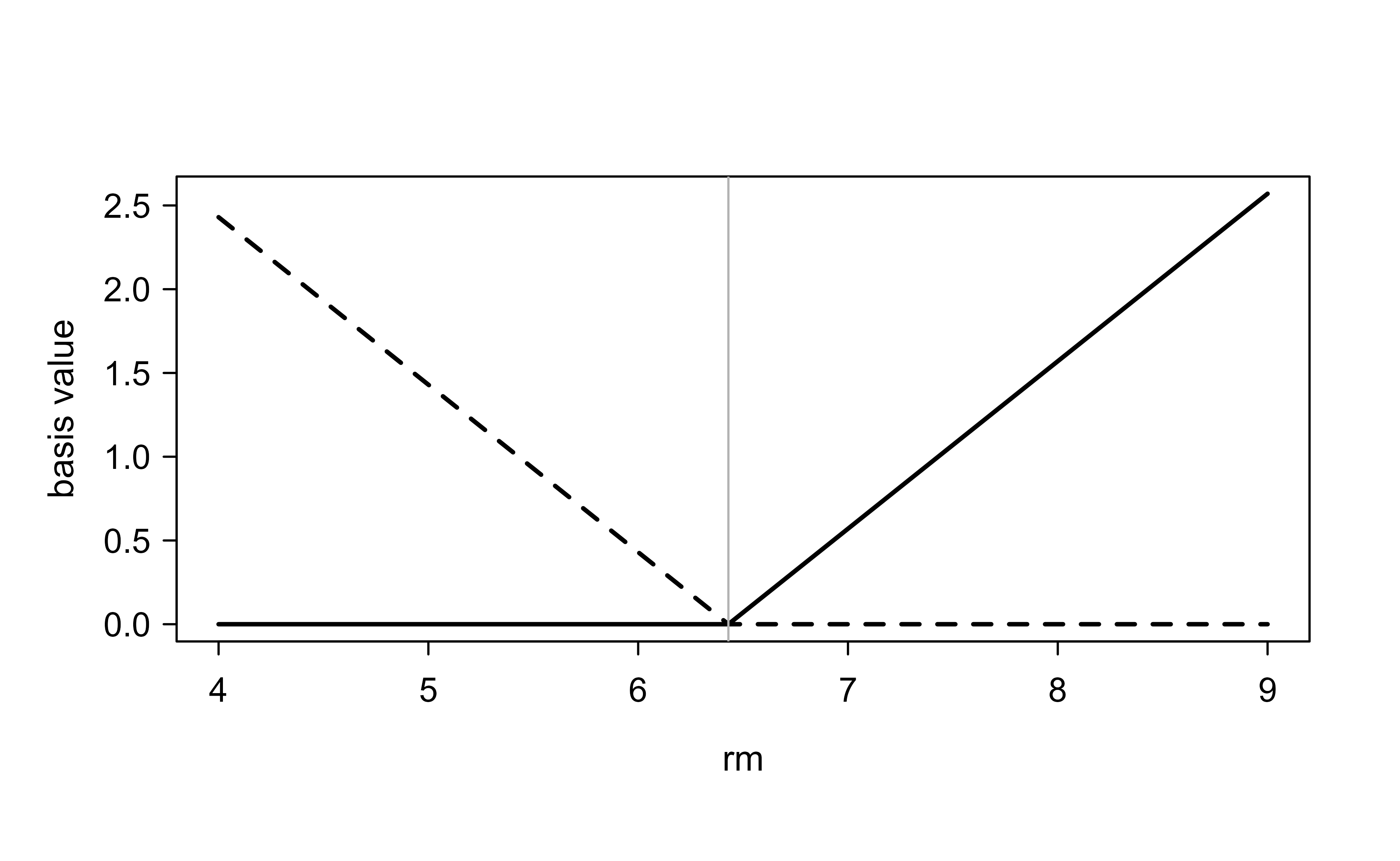
In the summary, each row is a hinge term such as h(rm-6.43), the positive part $(rm - 6.43)_+$ — zero until the average number of rooms rm exceeds 6.43, then rising linearly. That single number is where the fitted curve bends. The hinge and its mirror image are the whole vocabulary MARS builds from:

Show code

x <- seq(4, 9, 0.01)
plot(x, pmax(x - 6.43, 0), type = "l", lwd = 2, ylab = "basis value", xlab = "rm")
lines(x, pmax(6.43 - x, 0), lwd = 2, lty = 2)
abline(v = 6.43, col = "grey70")

A hinge h(x - 6.43) = (x - 6.43)+ and its reflection. MARS adds such pairs at data-chosen knots and multiplies them for interactions.

Reading the selected terms tells you directly where each predictor bends and which predictors interact — a large part of why MARS stays interpretable. And the flexibility is not free decoration: against a plain linear model, the data-chosen bends pay off in honest out-of-sample error. A 5-fold cross-validation makes the comparison concrete:

Show code

set.seed(1); folds <- sample(rep(1:5, length.out = nrow(Boston)))
cv_rmse <- function(fit_fn) sqrt(mean(sapply(1:5, function(k) {
  tr <- Boston[folds != k, ]; te <- Boston[folds == k, ]
  mean((predict(fit_fn(tr), te) - te$medv)^2)
})))
c(MARS   = cv_rmse(function(d) earth(medv ~ ., data = d, degree = 2)),
  linear = cv_rmse(function(d) lm(medv ~ ., data = d)))
#>     MARS   linear 
#> 3.761013 4.872735

MARS cuts the cross-validated error against ordinary least squares by roughly a fifth, because the housing relationships genuinely bend (the value of an extra room rises sharply only past a threshold) and interact (the penalty for a high lower-status percentage depends on the neighborhood). It buys that flexibility while staying additive and readable — the GCV criterion developed above having already pruned the model back to the terms that earn their keep, so you are not paying for the flexibility in variance.

Theoretical properties

The ANOVA decomposition

Because each term is a product of hinges in distinct variables, the fitted MARS model collects naturally into a functional ANOVA decomposition. Group the terms by the set of variables they involve:

\[ \hat{f}(X) = \beta_0 + \sum_{j} f_j(X_j) + \sum_{j<k} f_{jk}(X_j, X_k) + \sum_{j<k<l} f_{jkl}(X_j, X_k, X_l) + \cdots, \tag{9.6}\]

where $f_j$ collects all terms involving only $X_j$ (a one-dimensional piecewise-linear curve), $f_{jk}$ collects all terms that are products in exactly $X_j$ and $X_k$ (a two-dimensional surface), and so on. The degree hyperparameter caps the highest order present: degree = 1 keeps only the main-effect terms $f_j$ and yields a purely additive model, degree = 2 adds pairwise surfaces, and so forth. This decomposition is the formal reason MARS is interpretable: one can plot each $f_j$ and each $f_{jk}$ separately and read off where the response bends and which pairs of variables interact. It also explains the additive penalty choice $c = 2$, since restricting to Equation 9.6 at first order shrinks the candidate space the forward search explores.

Connections to other methods

MARS sits at the intersection of several methods covered elsewhere. With degree = 1 and the hierarchy convention it is a forward-stagewise additive model in a linear-spline basis, closely related to the additive splines of Chapter 6, but with knots chosen adaptively rather than fixed. As noted earlier, with hinges replaced by step indicators and parents made non-reusable it reduces exactly to CART (Chapter 8); MARS can be read as “CART with continuous, reusable basis functions,” which is precisely what lets it represent smooth additive structure that a single tree fits poorly. The forward greedy search is the same matching-pursuit idea that underlies boosting (Chapter 12): both repeatedly append the basis element most correlated with the current residual. The difference is that MARS refits all coefficients by least squares at every step (it is fully corrective) and then prunes, whereas gradient boosting takes small shrunken steps and never deletes, which is one reason boosting generalizes better while MARS stays more interpretable.

Bias, variance, and complexity

The forward to backward to GCV pipeline is a bias-variance control device. Increasing the number of terms (or degree) lowers approximation bias by enriching the spline basis but raises variance, since each adaptively chosen knot fits noise as well as signal; the inflated parameter count $r + cK$ in GCV is what arrests this before variance dominates. Adaptive knot selection means MARS can achieve low bias in regions where the true function bends sharply while spending few parameters in flat regions, which is its main statistical advantage over a fixed-knot basis.

Computationally, one forward step costs $O(n\,p\,|M|)$: for each of the $|M|$ parents and $p$ variables, an $O(n)$ knot scan using the incremental updates of Equation 9.2. Running the forward pass to $M_{\max}$ terms therefore costs roughly $O(n\,p\,M_{\max}^2)$, and the backward pass adds $O(M_{\max}^3)$ for the deletion sequence. Memory is dominated by the $n \times M_{\max}$ design matrix. The quadratic dependence on $M_{\max}$ is the practical limit on model size.

Failure modes

When MARS breaks

The greedy forward search is myopic: it can miss an interaction whose two parents are individually useless but jointly predictive (a pure interaction with no main effects), because neither parent will be selected first. The fast.k and parent-eligibility heuristics in earth trade accuracy for speed and can worsen this. MARS is also sensitive to correlated predictors, since it may pick an arbitrary one of several near-duplicate columns, making the selected variable set unstable across resamples. Hinge fits extrapolate linearly beyond the outermost knot, so predictions far outside the training range can grow without bound, and a knot placed near a sparse boundary region produces high-variance, sometimes wild, behavior there. Finally, GCV depends on the penalty $c$; if $c$ is set too small the model is consistently overfit, and on heteroscedastic or heavy-tailed noise the GCV size estimate degrades because it assumes constant-variance errors.

Practical guidance

Hyperparameters and how to choose them

The few knobs that matter, in the earth parameterization, are:

degree (maximum interaction order). Start with degree = 1 (additive) as a baseline and try degree = 2 to allow pairwise interactions. Going beyond degree = 3 is rarely worthwhile and hurts interpretability and stability. Choose by cross-validated error rather than GCV when interaction order is in doubt, since GCV is itself only an approximation.
nk (maximum number of terms in the forward pass, the $M_{\max}$ above). The default in earth is roughly $\min(200, \max(20, 2p)) + 1$. It must be large enough that the forward pass overshoots the eventual model; if the selected size equals nk the model is being truncated and nk should be raised.
penalty (the GCV per-knot cost $c$). Defaults to $3$ for degree > 1 and $2$ for additive models. Increase it to force a sparser, smoother model; setting it to $0$ disables the knot penalty and tends to overfit.
thresh and minspan/endspan. thresh is the minimum relative RSS improvement required to keep adding terms (a forward-pass stopping rule). minspan controls the minimum number of observations between adjacent knots, which prevents knots from chasing individual points; the default uses Friedman’s formula scaling with $\log n$. Increasing minspan regularizes against boundary instability.

Diagnostics

Use plotmo() to view the fitted $f_j$ and $f_{jk}$ surfaces from Equation 9.6, plot() on the fitted object for residual and model-selection diagnostics (the GCV curve against model size should show a clear minimum, not a truncation at nk), and evimp() for variable importance as shown in the example. To assess stability under correlated predictors, refit on bootstrap resamples and check whether the selected variables and knot locations are consistent. Always sanity-check predictions near and beyond the data boundary, where linear extrapolation can mislead.

Tip

Because the entire forward to backward search is fast, wrapping earth in an outer cross-validation loop (refitting the whole pipeline on each fold) is affordable and gives a more honest error estimate than GCV alone, especially for choosing degree. The nfold argument to earth does exactly this.

Strengths and limitations

MARS earns its place through a few genuine advantages, summarized here.

Locality. A major advantage of these piecewise linear basis functions is that they are “local,” meaning each is non-zero in only a small portion of the feature space, even when several are multiplied together. This locality is what makes model fitting practical in high dimensions.
Computational efficiency. It takes on the order of $n$ operations to try every knot at each step of the process, for each of the $j = 1, \dots, p$ variables, so the adaptive search is affordable.
Readable structure. When higher-order products are in the model, the convention is to also include the corresponding lower-order components. Strictly speaking this is not required, but it is good modeling practice and keeps the fitted model interpretable.³
Extends to classification. MARS can be applied to classification problems, for instance by coding the response as 0 and 1, though doing so is somewhat artificial. There are dedicated MARS-like algorithms designed specifically for classification.

It also has clear limitations to keep in mind.

Warning

Each input can appear at most once in any given product, so higher-order powers of a single input (such as $X_1^2$ via $(X_1 - t)_+ \times (X_1 - s)_+$ on the same variable) are not allowed. Permitting them tends to produce unstable fits, especially near the boundaries of the data.

You can also cap the complexity of interactions directly, restricting products to a chosen maximum order (for example, only second-degree or third-degree interactions). This is the degree argument in the worked example above.

When to use this

Reach for MARS when you want an automatic, interpretable model that captures nonlinearities and a modest number of interactions across many predictors, and you value being able to read off where the relationships bend. If raw predictive accuracy is the only goal, a tuned gradient boosting model (Chapter 12) will often do better, at the cost of interpretability.

MARS was introduced by Jerome Friedman in 1991. The name “MARS” is trademarked, which is why the popular R implementation is called earth rather than mars.↩︎
Selecting a knot location from the data spends model flexibility even though it does not add a coefficient in the usual sense. GCV charges for this through the term $cK$ below, otherwise the penalty would understate the true complexity and GCV would favor models that are too large.↩︎
This is the same “hierarchy” or “marginality” principle you see in classical regression: if an interaction $X_1 X_2$ is in the model, the main effects $X_1$ and $X_2$ usually belong there too.↩︎

# Multivariate Adaptive Regression Splines {#sec-mars} ```{r} #| include: false source("_common.R") ``` Imagine you want to predict a house price from dozens of features (square footage, lot size, year built, neighborhood, and so on), and you suspect the relationship is not a straight line. Square footage might matter a lot up to a point and then flatten out; the effect of one feature might depend on the value of another. Plain linear regression cannot capture these bends and interactions on its own, and fitting a separate smooth curve to each predictor by hand quickly becomes unmanageable when there are many inputs. Multivariate Adaptive Regression Splines (MARS) is a method that handles exactly this situation automatically. It builds a regression model out of simple "hinge" pieces, lines that bend at chosen locations, and it decides on its own where to put the bends, which predictors to use, and which predictors should interact. In this sense MARS sits between two ideas you have already met: it generalizes stepwise linear regression by letting the model add bent (not just straight) terms, and it can be seen as a modification of the CART procedure from the classification and regression trees chapter (@sec-regression-trees) that performs better in the regression setting.^[MARS was introduced by Jerome Friedman in 1991. The name "MARS" is trademarked, which is why the popular R implementation is called `earth` rather than `mars`.] By the end of this chapter you will understand the building blocks MARS uses (piecewise linear basis functions, called hinge functions), how the forward, then backward, model-building strategy works, and how the method chooses a final model size. You will also see a short worked example. The core machinery is an expansion in the piecewise linear basis function family. ::: {.callout-note} MARS is not used as much today as it once was, having been largely overtaken by tree ensembles such as gradient boosting (@sec-gradient-boosting). It remains worth studying because its ideas, adaptive knot selection and automatic interaction discovery, are clear and instructive, and the model it produces is unusually easy to interpret. ::: ## How MARS relates to CART {-} It helps to anchor MARS against CART, since the two share a common spirit but differ in their building blocks. CART splits the feature space with step functions and produces a binary tree; MARS replaces those hard steps with gentle bends and allows more flexible structure. To see the connection, picture starting from a tree-style procedure and making the following changes: - Replace the piecewise linear basis function with step functions (for example, $I(x-t>0)$ and $I(x-t) \le 0$). - When a model term is multiplied by a candidate term, it gets replaced by the resulting interaction and is therefore no longer available for further interaction. With those two changes, the MARS forward procedure becomes essentially the CART tree-growing algorithm. Multiplying a step function by a pair of reflected step functions is equivalent to splitting a node at that step, and the second restriction (a node may not be split more than once) is what forces the binary tree structure. MARS is more flexible precisely because it drops these restrictions: it keeps smooth hinge functions instead of hard steps, and it allows additive structures rather than being confined to a binary tree. ::: {.callout-important title="Key idea"} CART is a special, restricted case of the MARS-style construction. Loosening the restrictions (smooth hinges, reusable terms) is what gives MARS its extra power and its ability to represent additive effects. ::: ## The building blocks: hinge functions {-} The atom of a MARS model is a one-sided linear piece. Consider a basis function of the following form, where the "+" subscript means "positive part" with a knot at $t$: $$ (x-t)_+ = \begin{cases} x-t & \text{ if } x > t \\ 0 & \text{otherwise} \end{cases} $$ and its mirror image, $$ (t-x)_+ = \begin{cases} t- x & \text{ if } x < t \\ 0 & \text{otherwise} \end{cases} $$ Each of these is flat (equal to zero) on one side of the knot $t$ and rises linearly on the other side. They are linear splines, and because one is the mirror image of the other across $t$, the pair is called a reflected pair. ::: {.callout-tip title="Intuition"} A single hinge function is a "ramp" that switches on at $t$. A reflected pair gives you one ramp going up to the right of $t$ and one going up to the left of $t$. Adding both to a model lets the fitted curve bend at $t$ and take a different slope on each side, which is how MARS turns straight lines into flexible, piecewise-linear shapes. ::: Where do we put the knots? MARS forms such a reflected pair for each input $X_j$ with knots placed at every observed value $x_{ij}$ of that input. This is what makes the knot placement adaptive: instead of guessing knot locations in advance, the method considers every data point as a candidate. The full collection of basis functions is $$ C = \{(X_j - t)_+ , (t-X_j)_+\}_{t \in \{x_{1j}, \dots, x_{nj} \}}, j = 1, \dots, p $$ If all input values are distinct, this collection can contain as many as $2np$ basis functions, which can be very large. ## The model and how it is built {-} A MARS model has the form $$ f(X) = \beta_0 + \sum_{m=1}^M \beta_m h_m (X) $$ where each $h_m(X)$ is either a function drawn from the collection $C$ or a product of two or more such functions. Products are what create interactions between variables. As in forward stepwise linear regression, we build the final model from these transformed inputs rather than from the original inputs directly. Once the set of terms $h_m$ is fixed, estimating the coefficients $\beta_m$ is the easy part: we use ordinary least squares, minimizing the residual sum of squares. The hard and important part is choosing which $h_m(X)$ to include, and that is where the adaptive search comes in. ### Formulation: the regression problem MARS solves {-} Fix the structure of the model, that is, the list of terms $h_0 \equiv 1, h_1, \dots, h_M$. Collect them into the $n \times (M+1)$ design matrix $\mathbf{B}$ with entries $B_{im} = h_m(x_i)$, so column $0$ is a column of ones. Stacking the responses into $\mathbf{y} \in \mathbb{R}^n$ and the coefficients into $\boldsymbol\beta = (\beta_0, \beta_1, \dots, \beta_M)^\top$, MARS solves the ordinary least squares problem $$ \hat{\boldsymbol\beta} = \arg\min_{\boldsymbol\beta} \; \big\| \mathbf{y} - \mathbf{B}\boldsymbol\beta \big\|_2^2 = (\mathbf{B}^\top \mathbf{B})^{-1} \mathbf{B}^\top \mathbf{y}, $$ {#eq-MARS-ols} with fitted values $\hat{\mathbf{y}} = \mathbf{B}\hat{\boldsymbol\beta} = \mathbf{H}\mathbf{y}$ and hat matrix $\mathbf{H} = \mathbf{B}(\mathbf{B}^\top \mathbf{B})^{-1}\mathbf{B}^\top$. The statistical model behind @eq-MARS-ols is the usual one, $y_i = f(x_i) + \varepsilon_i$ with $\mathbb{E}[\varepsilon_i] = 0$ and $\mathrm{Var}(\varepsilon_i) = \sigma^2$, and $f$ assumed to lie (approximately) in the span of products of hinge functions. The space of functions reachable by MARS is the linear span of the constant together with all products $\prod_{k} (\pm(X_{j_k} - t_k))_+$ that respect two structural constraints stated later: each variable appears at most once in a product, and (by convention) lower-order parts of any product are also present. Within that span the fit is linear in $\boldsymbol\beta$, so for a fixed structure everything reduces to least squares; the difficulty, and all of the adaptivity, is in choosing the structure. ### The forward pass: adding terms greedily {-} We start as simply as possible. The model begins with the constant function $h_0(X) = 1$, and every function in $C$ is a candidate to be added next. At each stage, we consider every product of a function $h_l$ already in the current model set $M$ with one of the reflected pairs in $C$, that is, terms of the form $$ \hat{\beta}_{M + 1} h_l(X) \times (X_j -t)_+ + \hat{\beta}_{M + 2} h_l(X) \times (t - X_j )_+, h_l \in M $$ where $h_l$ is some basis function already in the model. Among all such candidate additions, we pick the one that produces the largest decrease in training error, and we add that reflected pair of products to the model set $M$. ::: {.callout-note} Because each new term is a product of an existing term with a new reflected pair, the search naturally discovers interactions. Multiplying by the constant $h_0(X) = 1$ keeps the new term as a simple main effect; multiplying by an existing hinge creates a two-way (or higher) interaction. ::: To make this concrete, here is how the first couple of stages play out. First, we consider adding a function of the form $\beta_1 (X_j - t)_+ + \beta_2(t-X_j)_+, t \in \{ x_{ij} \}$ (multiplying by the constant function just produces the reflected pair itself). Suppose that for a particular data set the best choice turns out to be $\hat{\beta}_1 (X_2 - x_{72})_+ + \hat{\beta}_2 (x_{72} - X_2)_+$. We add this to the set $M$. Next, we consider adding a pair of products of the form $$ h_m (X) \times (X_j - t)_+ $$ $$ h_m(X) \times (t- X_j)_+, t \in \{ x_{ij} \} $$ where for $h_m$ we now have three choices: $$ h_0(X) = 1, h_1(X) = (X_2 - x_{72})_+ $$ or $$ h_2(X) = (x_{72} - X_2)_+ $$ For example, the third choice can produce an interaction term such as $(X_1 - x_{51})_+ \times (x_{72} - X_2)_+$. The forward pass continues until a pre-specified number of terms is in the model. By design this gives a large model that overfits the data, which is exactly what we want before pruning. ### Derivation: the gain from adding a reflected pair {-} It is worth seeing exactly what quantity the forward pass maximizes, because it explains why the search is only $O(n)$ per variable and why knots can be tested incrementally. Suppose the current model has design matrix $\mathbf{B}$ and projects $\mathbf{y}$ onto $\mathrm{col}(\mathbf{B})$, leaving residual $\mathbf{r} = \mathbf{y} - \mathbf{B}\hat{\boldsymbol\beta} = (\mathbf{I} - \mathbf{H})\mathbf{y}$. We consider adding the two new columns $\mathbf{u}(t) = h_l \odot (X_j - t)_+$ and $\mathbf{v}(t) = h_l \odot (t - X_j)_+$ (elementwise products evaluated at the data, for a fixed parent $h_l$, variable $j$, and knot $t$). The decrease in residual sum of squares from appending columns $\mathbf{Z} = [\mathbf{u}(t), \mathbf{v}(t)]$ to a model that already contains $\mathbf{B}$ is, by the standard formula for the extra sum of squares of a projection onto the orthogonal complement, $$ \Delta \mathrm{RSS}(j,t,l) = \tilde{\mathbf{Z}}^\top \mathbf{r} \,\big( \tilde{\mathbf{Z}}^\top \tilde{\mathbf{Z}} \big)^{-1} \tilde{\mathbf{Z}}^\top \mathbf{r}, \qquad \tilde{\mathbf{Z}} = (\mathbf{I} - \mathbf{H})\mathbf{Z}, $$ {#eq-MARS-gain} where $\tilde{\mathbf{Z}}$ is $\mathbf{Z}$ orthogonalized against the existing columns. To see @eq-MARS-gain, write the augmented projection in block form: regressing $\mathbf{y}$ on $[\mathbf{B}, \mathbf{Z}]$ is equivalent, by the Frisch to Waugh to Lovell theorem, to first removing $\mathbf{B}$ from both $\mathbf{y}$ and $\mathbf{Z}$ and then regressing the residual $\mathbf{r}$ on $\tilde{\mathbf{Z}}$. The reduction in RSS achieved by that second regression is the squared length of the projection of $\mathbf{r}$ onto $\mathrm{col}(\tilde{\mathbf{Z}})$, namely $\mathbf{r}^\top \tilde{\mathbf{Z}} (\tilde{\mathbf{Z}}^\top \tilde{\mathbf{Z}})^{-1} \tilde{\mathbf{Z}}^\top \mathbf{r}$, which is @eq-MARS-gain. The forward pass selects the triple $(j,t,l)$ maximizing this gain, which is the same as choosing the candidate that minimizes the new training RSS, since the old RSS is fixed. Two facts make this cheap. First, only $\mathbf{r}$ enters, so the parent fit is computed once per stage. Second, as the knot $t$ sweeps through the sorted values $x_{(1)j} > x_{(2)j} > \dots$ of variable $j$, the column $(X_j - t)_+$ changes by a simple, incremental amount: lowering the knot past one data point adds a constant slope contribution over the points already to the right of $t$. The inner products $\tilde{\mathbf{Z}}^\top \mathbf{r}$ and the small Gram matrix $\tilde{\mathbf{Z}}^\top \tilde{\mathbf{Z}}$ can therefore be updated in $O(1)$ per knot using running sums, giving $O(n)$ work to scan all knots of one variable rather than the naive $O(n^2)$. This is the precise sense of the locality and efficiency claims made later. ::: {.callout-tip title="Intuition"} The strategy is deliberately "grow too big, then trim." Greedily adding terms is fast but tends to keep some terms that only help on the training set. Pruning afterward removes them. ::: ### The backward pass: pruning {-} To undo the overfitting, MARS uses backward deletion. At each step it removes the single term whose removal causes the smallest increase in residual squared error. Running this all the way down produces, for each model size $\lambda$ (the number of terms), an estimated "best" model $\hat{f}_\lambda$ of that size. The cost of deleting a term mirrors @eq-MARS-gain. If $\mathbf{B}$ is the current design and we drop column $m$, leaving $\mathbf{B}_{-m}$, the increase in RSS equals the squared length of the part of $\hat{\mathbf{y}}$ that $\mathbf{B}_{-m}$ cannot recover. Writing $\hat\beta_m$ for the fitted coefficient of column $m$ and $\mathbf{w}_m = (\mathbf{I} - \mathbf{H}_{-m})\mathbf{b}_m$ for column $m$ orthogonalized against the others (where $\mathbf{b}_m$ is the $m$th column and $\mathbf{H}_{-m}$ the hat matrix of $\mathbf{B}_{-m}$), $$ \Delta \mathrm{RSS}_{\text{drop } m} = \hat\beta_m^2 \, \|\mathbf{w}_m\|_2^2 . $$ {#eq-MARS-drop} Backward deletion removes, at each step, the surviving term with the smallest value of @eq-MARS-drop (the constant $h_0$ is never removed). The asymmetry with the forward pass is deliberate: the forward pass must add reflected pairs to keep the candidate set rich, but backward deletion removes terms one at a time, so it can keep a useful "up" hinge while discarding its unused mirror image. ## Choosing the model size {-} We are left with a sequence of candidate models of different sizes and must pick one. Cross-validation would work but is computationally expensive here, because we would have to repeat the entire forward-backward search on each fold. Instead, MARS uses generalized cross-validation (GCV), a closed-form approximation: $$ GCV(\lambda) = \frac{\sum_{i=1}^n (y_i - \hat{f}_\lambda(x_i))^2}{(1- M(\lambda)/n)^2} $$ The numerator is just the training residual sum of squares; the denominator penalizes model complexity, so GCV trades off fit against the number of effective parameters. Here $M(\lambda)$ is the effective number of parameters in the model, which accounts both for the parameters in the model and for the cost of having searched over knot positions.^[Selecting a knot location from the data spends model flexibility even though it does not add a coefficient in the usual sense. GCV charges for this through the term $cK$ below, otherwise the penalty would understate the true complexity and GCV would favor models that are too large.] In practice the effective parameter count is taken to be $M(\lambda) = r + cK$. The three quantities are: - $r$: the number of linearly independent basis functions in the model. - $K$: the number of knots selected during the forward process. - $c$: a per-knot penalty, typically $c = 3$, or $c = 2$ if the model is restricted to be additive (no interactions). We then choose the size $\lambda$ that minimizes $GCV(\lambda)$. ### Why GCV approximates cross-validation {-} GCV is not an arbitrary penalty; it is a computable surrogate for leave-one-out cross-validation. For a linear smoother $\hat{\mathbf{y}} = \mathbf{H}\mathbf{y}$ with a fixed structure, the leave-one-out residual has the well known closed form $$ y_i - \hat{f}^{(-i)}(x_i) = \frac{y_i - \hat{f}(x_i)}{1 - H_{ii}}, $$ {#eq-MARS-loocv} so the leave-one-out error is $\frac{1}{n}\sum_i \big( (y_i - \hat{f}(x_i)) / (1 - H_{ii}) \big)^2$. GCV replaces each leverage $H_{ii}$ by the average leverage $\frac{1}{n}\,\mathrm{tr}(\mathbf{H}) = \mathrm{tr}(\mathbf{H})/n$, which turns @eq-MARS-loocv into $$ \mathrm{GCV} = \frac{1}{n} \frac{\sum_{i=1}^n (y_i - \hat{f}(x_i))^2}{\big(1 - \mathrm{tr}(\mathbf{H})/n\big)^2}. $$ {#eq-MARS-gcv-derived} For a least squares fit with $r$ independent columns, $\mathrm{tr}(\mathbf{H}) = r$, which recovers the denominator $(1 - r/n)^2$. The numerator above is the mean residual sum of squares rather than the total; the version in the text drops the leading $1/n$, which does not change the minimizing $\lambda$. The one extra ingredient particular to MARS is that knot selection consumes degrees of freedom that the ordinary trace does not see: each of the $K$ knots was chosen by searching over the data, behaving empirically like roughly $c$ additional fitted parameters. Replacing $\mathrm{tr}(\mathbf{H}) = r$ by the inflated count $M(\lambda) = r + cK$ is exactly this correction, and it is why GCV here charges for the search and not only for the coefficients. Without it, GCV would systematically prefer models that are too large. ::: {.callout-note} The substitution of the mean leverage $\mathrm{tr}(\mathbf{H})/n$ for the individual $H_{ii}$ is what makes GCV invariant to rotations of the response and removes the need to compute the full hat matrix. It is exact when all leverages are equal and a good approximation otherwise, which is the same justification used for GCV in smoothing splines and ridge regression. ::: The leave-one-out shortcut @eq-MARS-loocv is the load-bearing step, so it is worth confirming numerically on a small linear fit (the same identity MARS relies on for any fixed structure). ```{r mars-loocv-check} #| eval: false set.seed(1) n <- 40 X <- cbind(1, matrix(rnorm(n * 3), n, 3)) # fixed design y <- X %*% c(1, 2, -1, 0.5) + rnorm(n) H <- X %*% solve(crossprod(X), t(X)) # hat matrix res <- as.numeric(y - H %*% y) # ordinary residuals shortcut <- res / (1 - diag(H)) # via eq-MARS.qmd-loocv # brute-force leave-one-out residuals brute <- sapply(seq_len(n), function(i) { fit <- lm.fit(X[-i, ], y[-i]) y[i] - sum(X[i, ] * fit$coefficients) }) max(abs(shortcut - brute)) # ~ 1e-13 ``` ::: {.callout-tip} If you constrain MARS to additive models (no products of hinge functions), use $c = 2$. The smaller penalty reflects the fact that an additive search explores fewer candidate structures, so each knot costs less complexity. ::: ## A worked example {-} The `earth` package provides the standard R implementation of MARS. We fit it to the Boston housing data, predicting median home value `medv` from the other variables, with `degree = 2` so the forward pass may multiply two hinges and capture interactions: ```{r mars-earth, message = FALSE, warning = FALSE} library(earth) data(Boston, package = "MASS") mars_fit <- earth(medv ~ ., data = Boston, degree = 2) summary(mars_fit) # GCV-selected hinge terms and model size evimp(mars_fit) # which variables earned their place ``` In the summary, each row is a hinge term such as `h(rm-6.43)`, the positive part $(rm - 6.43)_+$ --- zero until the average number of rooms `rm` exceeds 6.43, then rising linearly. That single number is where the fitted curve *bends*. The hinge and its mirror image are the whole vocabulary MARS builds from: ```{r mars-hinge} #| fig-cap: "A hinge h(x - 6.43) = (x - 6.43)+ and its reflection. MARS adds such pairs at data-chosen knots and multiplies them for interactions." x <- seq(4, 9, 0.01) plot(x, pmax(x - 6.43, 0), type = "l", lwd = 2, ylab = "basis value", xlab = "rm") lines(x, pmax(6.43 - x, 0), lwd = 2, lty = 2) abline(v = 6.43, col = "grey70") ``` Reading the selected terms tells you directly where each predictor bends and which predictors interact --- a large part of why MARS stays interpretable. And the flexibility is not free decoration: against a plain linear model, the data-chosen bends pay off in honest out-of-sample error. A 5-fold cross-validation makes the comparison concrete: ```{r mars-cv} set.seed(1); folds <- sample(rep(1:5, length.out = nrow(Boston))) cv_rmse <- function(fit_fn) sqrt(mean(sapply(1:5, function(k) { tr <- Boston[folds != k, ]; te <- Boston[folds == k, ] mean((predict(fit_fn(tr), te) - te$medv)^2) }))) c(MARS = cv_rmse(function(d) earth(medv ~ ., data = d, degree = 2)), linear = cv_rmse(function(d) lm(medv ~ ., data = d))) ``` MARS cuts the cross-validated error against ordinary least squares by roughly a fifth, because the housing relationships genuinely bend (the value of an extra room rises sharply only past a threshold) and interact (the penalty for a high lower-status percentage depends on the neighborhood). It buys that flexibility while staying additive and readable --- the GCV criterion developed above having already pruned the model back to the terms that earn their keep, so you are not paying for the flexibility in variance. ## Theoretical properties {-} ### The ANOVA decomposition {-} Because each term is a product of hinges in distinct variables, the fitted MARS model collects naturally into a functional ANOVA decomposition. Group the terms by the set of variables they involve: $$ \hat{f}(X) = \beta_0 + \sum_{j} f_j(X_j) + \sum_{j<k} f_{jk}(X_j, X_k) + \sum_{j<k<l} f_{jkl}(X_j, X_k, X_l) + \cdots, $$ {#eq-MARS-anova} where $f_j$ collects all terms involving only $X_j$ (a one-dimensional piecewise-linear curve), $f_{jk}$ collects all terms that are products in exactly $X_j$ and $X_k$ (a two-dimensional surface), and so on. The `degree` hyperparameter caps the highest order present: `degree = 1` keeps only the main-effect terms $f_j$ and yields a purely additive model, `degree = 2` adds pairwise surfaces, and so forth. This decomposition is the formal reason MARS is interpretable: one can plot each $f_j$ and each $f_{jk}$ separately and read off where the response bends and which pairs of variables interact. It also explains the additive penalty choice $c = 2$, since restricting to @eq-MARS-anova at first order shrinks the candidate space the forward search explores. ### Connections to other methods {-} MARS sits at the intersection of several methods covered elsewhere. With `degree = 1` and the hierarchy convention it is a forward-stagewise additive model in a linear-spline basis, closely related to the additive splines of @sec-gam, but with knots chosen adaptively rather than fixed. As noted earlier, with hinges replaced by step indicators and parents made non-reusable it reduces exactly to CART (@sec-regression-trees); MARS can be read as "CART with continuous, reusable basis functions," which is precisely what lets it represent smooth additive structure that a single tree fits poorly. The forward greedy search is the same matching-pursuit idea that underlies boosting (@sec-gradient-boosting): both repeatedly append the basis element most correlated with the current residual. The difference is that MARS refits all coefficients by least squares at every step (it is fully corrective) and then prunes, whereas gradient boosting takes small shrunken steps and never deletes, which is one reason boosting generalizes better while MARS stays more interpretable. ### Bias, variance, and complexity {-} The forward to backward to GCV pipeline is a bias-variance control device. Increasing the number of terms (or `degree`) lowers approximation bias by enriching the spline basis but raises variance, since each adaptively chosen knot fits noise as well as signal; the inflated parameter count $r + cK$ in GCV is what arrests this before variance dominates. Adaptive knot selection means MARS can achieve low bias in regions where the true function bends sharply while spending few parameters in flat regions, which is its main statistical advantage over a fixed-knot basis. Computationally, one forward step costs $O(n\,p\,|M|)$: for each of the $|M|$ parents and $p$ variables, an $O(n)$ knot scan using the incremental updates of @eq-MARS-gain. Running the forward pass to $M_{\max}$ terms therefore costs roughly $O(n\,p\,M_{\max}^2)$, and the backward pass adds $O(M_{\max}^3)$ for the deletion sequence. Memory is dominated by the $n \times M_{\max}$ design matrix. The quadratic dependence on $M_{\max}$ is the practical limit on model size. ### Failure modes {-} ::: {.callout-warning title="When MARS breaks"} The greedy forward search is myopic: it can miss an interaction whose two parents are individually useless but jointly predictive (a pure interaction with no main effects), because neither parent will be selected first. The `fast.k` and parent-eligibility heuristics in `earth` trade accuracy for speed and can worsen this. MARS is also sensitive to correlated predictors, since it may pick an arbitrary one of several near-duplicate columns, making the selected variable set unstable across resamples. Hinge fits extrapolate linearly beyond the outermost knot, so predictions far outside the training range can grow without bound, and a knot placed near a sparse boundary region produces high-variance, sometimes wild, behavior there. Finally, GCV depends on the penalty $c$; if $c$ is set too small the model is consistently overfit, and on heteroscedastic or heavy-tailed noise the GCV size estimate degrades because it assumes constant-variance errors. ::: ## Practical guidance {-} ### Hyperparameters and how to choose them {-} The few knobs that matter, in the `earth` parameterization, are: - `degree` (maximum interaction order). Start with `degree = 1` (additive) as a baseline and try `degree = 2` to allow pairwise interactions. Going beyond `degree = 3` is rarely worthwhile and hurts interpretability and stability. Choose by cross-validated error rather than GCV when interaction order is in doubt, since GCV is itself only an approximation. - `nk` (maximum number of terms in the forward pass, the $M_{\max}$ above). The default in `earth` is roughly $\min(200, \max(20, 2p)) + 1$. It must be large enough that the forward pass overshoots the eventual model; if the selected size equals `nk` the model is being truncated and `nk` should be raised. - `penalty` (the GCV per-knot cost $c$). Defaults to $3$ for `degree > 1` and $2$ for additive models. Increase it to force a sparser, smoother model; setting it to $0$ disables the knot penalty and tends to overfit. - `thresh` and `minspan`/`endspan`. `thresh` is the minimum relative RSS improvement required to keep adding terms (a forward-pass stopping rule). `minspan` controls the minimum number of observations between adjacent knots, which prevents knots from chasing individual points; the default uses Friedman's formula scaling with $\log n$. Increasing `minspan` regularizes against boundary instability. ### Diagnostics {-} Use `plotmo()` to view the fitted $f_j$ and $f_{jk}$ surfaces from @eq-MARS-anova, `plot()` on the fitted object for residual and model-selection diagnostics (the GCV curve against model size should show a clear minimum, not a truncation at `nk`), and `evimp()` for variable importance as shown in the example. To assess stability under correlated predictors, refit on bootstrap resamples and check whether the selected variables and knot locations are consistent. Always sanity-check predictions near and beyond the data boundary, where linear extrapolation can mislead. ::: {.callout-tip} Because the entire forward to backward search is fast, wrapping `earth` in an outer cross-validation loop (refitting the whole pipeline on each fold) is affordable and gives a more honest error estimate than GCV alone, especially for choosing `degree`. The `nfold` argument to `earth` does exactly this. ::: ## Strengths and limitations {-} MARS earns its place through a few genuine advantages, summarized here. - Locality. A major advantage of these piecewise linear basis functions is that they are "local," meaning each is non-zero in only a small portion of the feature space, even when several are multiplied together. This locality is what makes model fitting practical in high dimensions. - Computational efficiency. It takes on the order of $n$ operations to try every knot at each step of the process, for each of the $j = 1, \dots, p$ variables, so the adaptive search is affordable. - Readable structure. When higher-order products are in the model, the convention is to also include the corresponding lower-order components. Strictly speaking this is not required, but it is good modeling practice and keeps the fitted model interpretable.^[This is the same "hierarchy" or "marginality" principle you see in classical regression: if an interaction $X_1 X_2$ is in the model, the main effects $X_1$ and $X_2$ usually belong there too.] - Extends to classification. MARS can be applied to classification problems, for instance by coding the response as 0 and 1, though doing so is somewhat artificial. There are dedicated MARS-like algorithms designed specifically for classification. It also has clear limitations to keep in mind. ::: {.callout-warning} Each input can appear at most once in any given product, so higher-order powers of a single input (such as $X_1^2$ via $(X_1 - t)_+ \times (X_1 - s)_+$ on the same variable) are not allowed. Permitting them tends to produce unstable fits, especially near the boundaries of the data. ::: You can also cap the complexity of interactions directly, restricting products to a chosen maximum order (for example, only second-degree or third-degree interactions). This is the `degree` argument in the worked example above. ::: {.callout-tip title="When to use this"} Reach for MARS when you want an automatic, interpretable model that captures nonlinearities and a modest number of interactions across many predictors, and you value being able to read off where the relationships bend. If raw predictive accuracy is the only goal, a tuned gradient boosting model (@sec-gradient-boosting) will often do better, at the cost of interpretability. :::