Advanced Data Analysis

Nguyen, Mike

33 Association Rule Mining

Picture the checkout logs of a grocery store. Every receipt is a small, unordered set of items: someone bought bread, butter, and jam; someone else bought beer, chips, and diapers. There is no outcome variable, no label, no “right answer” to predict. Yet hidden in these millions of baskets are regularities a manager would love to know: people who buy bread and butter tend to buy jam, and that pattern repeats far more often than chance would allow. Association rule mining is the set of techniques for surfacing exactly these “if this, then that” patterns from large collections of co-occurrences, without anyone telling the algorithm in advance what to look for.

Because there is no target variable guiding the search, association rule mining belongs to unsupervised learning (Chapter 22), alongside cluster analysis (Chapter 23) and dimension reduction (Chapter 27). The difference is what we are looking for. Clustering groups observations (whole baskets) that resemble one another; association mining instead looks for co-occurrence among the items themselves, and reports its findings as human-readable rules rather than as a partition. The classic setting is market-basket analysis, but the same machinery describes which web pages are viewed together, which symptoms co-occur in patient records, and which words appear in the same document.

The whole subject rests on two questions we will make precise. First, which sets of items occur together often enough to be worth our attention (frequent itemset mining)? Second, among those frequent sets, which directional rules are both reliable and genuinely informative (rule generation and evaluation)? The reason the field exists as a separate discipline, rather than being a footnote to probability, is that the first question is computationally brutal: with $d$ distinct items there are $2^d - 1$ possible itemsets, and naive enumeration is hopeless. The central algorithmic insight, the Apriori principle, is what makes the search tractable.

Key idea

Association rule mining does not test a hypothesis you brought to the data. It searches an enormous space of possible patterns and reports the ones that pass thresholds you set. The thresholds (and the interest measure you choose) are the modeling decisions, and a rule with stellar confidence can still be worthless. We will see exactly why, and what to use instead.

33.1 The Market-Basket Model

We begin by fixing notation. Let $I = \{i_1, i_2, \dots, i_d\}$ be the set of all $d$ available items (the store’s catalog). A transaction $t$ is a subset of items, $t \subseteq I$, and the database is a collection of $n$ transactions $T = \{t_1, \dots, t_n\}$. An itemset $X$ is any subset of $I$; a $k$-itemset is one with $|X| = k$.

It is convenient to view the database as an $n \times d$ binary matrix, with rows indexing transactions and columns indexing items, where entry $(j, m)$ is $1$ if transaction $t_j$ contains item $i_m$ and $0$ otherwise. This makes the connection to ordinary tabular data explicit: market-basket data is just very wide, very sparse binary data, and the quantity that holds our pattern of zeros and ones is what every measure below counts.

The support count of an itemset $X$ is the number of transactions that contain it,

\[ \sigma(X) = \bigl| \{ t_j \in T : X \subseteq t_j \} \bigr|, \tag{33.1}\]

and its support is the fraction of transactions containing it,

\[ \operatorname{supp}(X) = \frac{\sigma(X)}{n} = \widehat{\Pr}(X \subseteq t). \tag{33.2}\]

The second equality is the bridge to probability and is worth stating plainly: if we draw a transaction at random from the database, $\operatorname{supp}(X)$ is the empirical probability that it contains all of $X$. Every interest measure in this chapter is ultimately a function of such empirical probabilities.

An association rule is an implication of the form $X \Rightarrow Y$, where $X$ and $Y$ are itemsets with $X \cap Y = \varnothing$. We call $X$ the antecedent (or left-hand side) and $Y$ the consequent (right-hand side). The rule is not a logical implication and not a causal claim; it is a statistical statement that transactions containing $X$ tend also to contain $Y$. Making “tend to” precise is the job of the next section.

33.2 Interest Measures

A rule $X \Rightarrow Y$ has two components we want to quantify: how often the pattern occurs at all, and how strongly the antecedent predicts the consequent. The first is support; the second is captured by a family of measures, each with a probabilistic reading and each with a characteristic blind spot.

33.2.1 Support and Confidence

The support of a rule is the support of the union of its two sides,

\[ \operatorname{supp}(X \Rightarrow Y) = \operatorname{supp}(X \cup Y) = \widehat{\Pr}(X \cup Y), \tag{33.3}\]

the empirical probability that a transaction contains every item in both $X$ and $Y$. Support measures how general a rule is: a rule with tiny support describes a corner case that may be a statistical fluke and is rarely actionable.

The confidence of a rule is the conditional empirical probability of the consequent given the antecedent,

\[ \operatorname{conf}(X \Rightarrow Y) = \frac{\operatorname{supp}(X \cup Y)}{\operatorname{supp}(X)} = \widehat{\Pr}(Y \mid X). \tag{33.4}\]

Confidence measures how reliable the rule is: among transactions that contain $X$, what fraction also contain $Y$. A confidence of $0.9$ for $\{\text{bread}, \text{butter}\} \Rightarrow \{\text{jam}\}$ says that nine of every ten butter-and-bread baskets also held jam.

Note

Confidence is exactly the maximum-likelihood estimate of $\Pr(Y \mid X)$ in the same sense that a sample proportion estimates a probability. This is why association mining is sometimes described as estimating a large collection of conditional probabilities and keeping only the sharp ones. The naive Bayes classifier (Chapter 18) rests on the same conditional-probability primitives, differing chiefly in that it has a designated label to condition toward.

33.2.2 Lift, Leverage, and Conviction

Confidence has a famous defect: it ignores how common the consequent is on its own. If $90\%$ of all baskets contain milk, then a rule “$\Rightarrow$ milk” with confidence $0.9$ tells us nothing, since we could achieve it by predicting milk for everyone. To correct for the baseline frequency of $Y$ we use lift, the ratio of the rule’s confidence to the unconditional support of the consequent,

\[ \operatorname{lift}(X \Rightarrow Y) = \frac{\operatorname{conf}(X \Rightarrow Y)}{\operatorname{supp}(Y)} = \frac{\operatorname{supp}(X \cup Y)}{\operatorname{supp}(X)\,\operatorname{supp}(Y)} = \frac{\widehat{\Pr}(X \cup Y)}{\widehat{\Pr}(X)\,\widehat{\Pr}(Y)}. \tag{33.5}\]

The last form makes the interpretation transparent. Lift is the ratio of the joint probability to the product of the marginals, so it compares the observed co-occurrence against what we would expect if $X$ and $Y$ were statistically independent. A value $\operatorname{lift} = 1$ means $X$ and $Y$ are independent (the rule carries no information beyond base rates); $\operatorname{lift} > 1$ means they appear together more than chance predicts (a positive association); and $\operatorname{lift} < 1$ means they appear together less than chance (a negative association). Lift is symmetric in $X$ and $Y$, which is both a virtue (it is a clean dependence measure) and a limitation (it forgets the rule’s direction).

Leverage measures the same departure from independence on an additive rather than multiplicative scale,

\[ \operatorname{leverage}(X \Rightarrow Y) = \operatorname{supp}(X \cup Y) - \operatorname{supp}(X)\,\operatorname{supp}(Y). \tag{33.6}\]

Leverage is the number of extra co-occurrences (as a fraction of the database) beyond the independence baseline. It is zero under independence and is bounded in $[-0.25, 0.25]$, which gives a sense of absolute effect size that lift lacks: a rule can have huge lift while leverage is negligible if both items are individually rare.

Conviction addresses confidence’s blind spot from the angle of implication failure,

\[ \operatorname{conviction}(X \Rightarrow Y) = \frac{1 - \operatorname{supp}(Y)}{1 - \operatorname{conf}(X \Rightarrow Y)} = \frac{\widehat{\Pr}(X)\,\widehat{\Pr}(\lnot Y)}{\widehat{\Pr}(X \cup \lnot Y)}. \tag{33.7}\]

The numerator is the frequency with which $Y$ is absent overall, and the denominator is the frequency with which the rule is “violated” (that is, $X$ present but $Y$ absent), so conviction is high when the rule is rarely broken relative to how often $Y$ is missing in general. Under independence conviction equals $1$; a logically perfect rule (confidence $1$, never violated) sends conviction to $\infty$. Unlike lift, conviction is directional, distinguishing $X \Rightarrow Y$ from $Y \Rightarrow X$, which often matters in practice.

Table 33.1: Interest measures for a rule $X \Rightarrow Y$, their probabilistic form, the value they take when $X$ and $Y$ are independent, and whether they distinguish the rule from its reverse.

Measure	Formula	Independence value	Direction-aware
Support	$\widehat{\Pr}(X \cup Y)$	(frequency)	no
Confidence	$\widehat{\Pr}(Y \mid X)$	$\operatorname{supp}(Y)$	yes
Lift	$\widehat{\Pr}(X \cup Y) / (\widehat{\Pr}(X)\widehat{\Pr}(Y))$	$1$	no
Leverage	$\widehat{\Pr}(X\cup Y) - \widehat{\Pr}(X)\widehat{\Pr}(Y)$	$0$	no
Conviction	$\widehat{\Pr}(X)\widehat{\Pr}(\lnot Y)/\widehat{\Pr}(X\cup\lnot Y)$	$1$	yes

Table 33.1 collects these together. No single measure dominates: confidence is interpretable but baseline-blind, lift is a clean dependence score but undirected and unstable for rare items, leverage gives absolute effect size, and conviction restores direction. Mature practice reports several and reads them together.

33.3 The Apriori Principle and Algorithm

We now confront the computational obstacle. To find all rules above given support and confidence thresholds, it suffices first to find all frequent itemsets, those $X$ with $\operatorname{supp}(X) \ge \operatorname{minsupp}$, and then to generate rules from them (next section). The trouble is that there are $2^d - 1$ candidate itemsets, an astronomically large number for a real catalog. We cannot count support for all of them. The Apriori principle is what saves us.

33.3.1 Downward Closure: A Derivation

The principle is a monotonicity statement about support, and it follows directly from the definition.

Apriori principle (downward closure)

If an itemset is frequent, then every one of its subsets is also frequent. Equivalently, if an itemset is infrequent, then every one of its supersets is also infrequent.

To prove it, let $X \subseteq Y$ be two itemsets, so $X$ is a subset of $Y$. Any transaction that contains $Y$ must, by definition of subset, contain $X$ as well. Therefore the set of transactions containing $Y$ is a subset of the set of transactions containing $X$, which gives

\[ \sigma(Y) \le \sigma(X) \quad\Longrightarrow\quad \operatorname{supp}(Y) \le \operatorname{supp}(X). \tag{33.8}\]

In words, support is anti-monotone: enlarging an itemset can only keep its support the same or shrink it, never raise it. Now suppose $X$ is infrequent, $\operatorname{supp}(X) < \operatorname{minsupp}$. For any superset $Y \supseteq X$, Equation 33.8 gives $\operatorname{supp}(Y) \le \operatorname{supp}(X) < \operatorname{minsupp}$, so $Y$ is infrequent too. This is the contrapositive of the principle, and it is the engine of pruning: the moment we find an itemset to be infrequent, we may discard all of its supersets without ever counting their support. Whole subtrees of the search space vanish at once.

33.3.2 The Apriori Algorithm

The Apriori algorithm (Agrawal and Srikant 1994) turns the principle into a breadth-first, level-wise search. It builds frequent itemsets of size $k$ only from frequent itemsets of size $k-1$, so an itemset is even considered (made a candidate) only if all of its immediate subsets already qualified.

Let $L_k$ denote the set of frequent $k$-itemsets and $C_k$ the set of candidate $k$-itemsets. The procedure is:

Initialize. Scan the database once to compute the support of every single item; keep those above $\operatorname{minsupp}$ as $L_1$.
Candidate generation. From $L_{k-1}$, form candidates $C_k$ by joining pairs of frequent $(k-1)$-itemsets that share their first $k-2$ items (the “join” step).
Prune. Remove from $C_k$ any candidate that has a $(k-1)$-subset not present in $L_{k-1}$. By downward closure such a candidate cannot be frequent, so we drop it before wasting a database scan on it (the “prune” step).
Count. Scan the database once to count the support of the surviving candidates in $C_k$; keep those above $\operatorname{minsupp}$ as $L_k$.
Repeat steps 2 to 4, incrementing $k$, until $L_k$ is empty. The frequent itemsets are $\bigcup_k L_k$.

Each level costs one pass over the data, so a database with maximum frequent-itemset size $k_{\max}$ requires about $k_{\max}+1$ passes. The work per pass is dominated by support counting, often implemented with a hash tree so that each transaction is matched against candidates efficiently. In the worst case (a very low threshold on dense data) the candidate set can still explode, but on the sparse, threshold-pruned itemsets typical of retail data Apriori is dramatically faster than brute force.

Warning

Apriori’s Achilles heel is candidate generation. When many itemsets clear the support threshold, $C_k$ can become enormous, and each database scan grows expensive. Repeatedly scanning a large database, once per level, is the practical bottleneck that motivated the next algorithm.

33.4 FP-Growth: Mining Without Candidate Generation

FP-growth (Han, Pei, and Yin 2000) attacks Apriori’s two costs (repeated scans and candidate explosion) by compressing the database into a tree and mining that tree directly, never generating candidates at all.

The idea proceeds in two passes. The first pass counts single-item supports and discards infrequent items, then fixes an ordering of the remaining frequent items by decreasing support. The second pass reads each transaction, drops its infrequent items, sorts the rest into the fixed order, and inserts the result as a path into a prefix tree called the FP-tree. Transactions that share a prefix share the upper portion of their path, and a counter on each node records how many transactions pass through it. Frequent items appearing in many baskets sit near the root and are stored once rather than repeatedly, so the tree is a compressed, lossless summary of all the frequency information needed. A header table links together all nodes for a given item, so the tree can be traversed by item.

Mining then works recursively and bottom-up. For each item (starting from the least frequent), the algorithm collects that item’s conditional pattern base, the set of prefix paths leading to it, weighted by counts, and builds a smaller conditional FP-tree from those paths. Frequent itemsets ending in that item are read off by recursing into the conditional tree. Because the patterns are grown by extending known frequent fragments rather than by proposing and testing candidates, FP-growth performs only two database scans total and avoids candidate generation entirely. The price is memory: the FP-tree must fit in RAM, and on dense data where little prefix sharing occurs the tree can be large. In broad strokes, Apriori trades memory for repeated computation while FP-growth trades computation for memory, and the better choice depends on data density and size.

33.5 Rule Generation and Pruning

Finding frequent itemsets answers the first question; we still must turn them into rules. The key observation is that a rule’s support is fixed once we choose the itemset, so support never has to be recomputed at this stage. For a frequent itemset $Z$, every rule of the form $X \Rightarrow Z \setminus X$ (for nonempty proper subsets $X \subset Z$) has the same support $\operatorname{supp}(Z)$, automatically above $\operatorname{minsupp}$. The only thing left to check is confidence.

This sets up a second pruning opportunity that mirrors downward closure. Consider moving an item from the antecedent to the consequent, that is, comparing $X \Rightarrow Z \setminus X$ against a rule with a smaller antecedent and larger consequent. Because the antecedent shrinks, its support can only grow (by Equation 33.8 applied to the antecedent), and since $\operatorname{conf} = \operatorname{supp}(Z)/\operatorname{supp}(\text{antecedent})$ with a fixed numerator, a larger denominator means smaller confidence. Formally, confidence is anti-monotone with respect to enlarging the consequent: if a rule with consequent $Y$ fails the confidence threshold, then every rule obtained from the same itemset by moving more items into the consequent also fails. We can therefore prune low-confidence rules level by level over consequent size, exactly as Apriori prunes itemsets, generating high-confidence rules without examining every subset split.

Once rules clear the confidence threshold, they are typically ranked and filtered by the additional interest measures of Table 33.1, most often lift, and frequently de-duplicated by removing redundant rules. A rule is redundant if a more general rule (one with the same or higher confidence and a subset antecedent) already exists, since the extra antecedent items add specificity without predictive gain.

33.6 Pitfalls: Why Confidence Is Not Enough

The single most important practical lesson is that high confidence does not imply a useful rule, and the reason is the baseline blindness we flagged earlier. The cleanest illustration is the classic tea-and-coffee example.

The high-confidence trap

Suppose $80\%$ of all customers buy coffee, and $25\%$ buy tea. Among tea buyers, $80\%$ also buy coffee. The rule $\{\text{tea}\} \Rightarrow \{\text{coffee}\}$ has confidence $0.80$, which sounds strong. But coffee is bought by $80\%$ of everyone, so buying tea does not raise the chance of buying coffee at all. The lift is $0.80 / 0.80 = 1$: tea and coffee are independent, and the rule is worthless despite its high confidence. In fact, if tea buyers bought coffee at $70\%$ (below the $80\%$ base rate), the rule would still have respectable confidence yet a lift of $0.875 < 1$, signaling a negative association that confidence alone completely hides.

This is why mature practice never ranks by confidence alone. Three further hazards deserve naming. First is multiple comparisons: an automated search over millions of candidate rules will, purely by chance, surface some with impressive statistics on any finite database, so apparent patterns demand validation on held-out data or correction for the number of rules examined. This is the same garden-of-forking-paths concern that haunts any large unsupervised search, and it connects to the broader project of interpretable machine learning (Chapter 35), where the goal is explanations one can actually trust. Second is the rare-item problem: a single global $\operatorname{minsupp}$ either drowns out interesting but infrequent items (set it high) or floods the output with noise (set it low). Third, and most fundamental, association is not causation: a rule $X \Rightarrow Y$ describes co-occurrence in a particular population and gives no license to conclude that stocking $X$ will sell more $Y$. The famous “beer and diapers” story, whatever its provenance, is at best a correlation discovered post hoc.

33.7 Demonstration

We work through two demonstrations. The first computes support, confidence, lift, leverage, and conviction entirely in base R on a tiny set of baskets, so that every formula above is visible as code. The second shows the standard production workflow with the arules package on the well-known Groceries dataset; it is displayed but not executed here, since arules may not be installed.

33.7.1 From Scratch in Base R

We hand-build a small grocery database as a binary transaction matrix and implement Equation 33.2 through Equation 33.7 directly. This is the runnable, verified portion.

Show code

# A tiny transaction database: rows = baskets, cols = items, 1 = present.
items <- c("bread", "butter", "jam", "milk", "beer")
baskets <- rbind(
  c(1, 1, 1, 0, 0),  # bread, butter, jam
  c(1, 1, 1, 1, 0),  # bread, butter, jam, milk
  c(1, 1, 0, 1, 0),  # bread, butter, milk
  c(1, 0, 0, 1, 0),  # bread, milk
  c(0, 0, 0, 1, 1),  # milk, beer
  c(1, 1, 1, 0, 0),  # bread, butter, jam
  c(0, 0, 0, 0, 1),  # beer
  c(1, 1, 1, 1, 1)   # everything
)
colnames(baskets) <- items
n <- nrow(baskets)

# supp(X): fraction of baskets containing every item in the set X.
supp <- function(X, data = baskets) {
  cols <- data[, X, drop = FALSE]
  mean(rowSums(cols) == length(X))
}

# All five interest measures for a rule X => Y.
rule_metrics <- function(X, Y, data = baskets) {
  sXY <- supp(c(X, Y), data); sX <- supp(X, data); sY <- supp(Y, data)
  conf <- sXY / sX
  data.frame(
    support    = sXY,
    confidence = conf,
    lift       = conf / sY,
    leverage   = sXY - sX * sY,
    conviction = if (conf < 1) (1 - sY) / (1 - conf) else Inf
  )
}

# Rule 1: {bread, butter} => {jam}  (expect strong, informative)
# Rule 2: {beer}          => {milk} (expect weak / near-independent)
r1 <- rule_metrics(c("bread", "butter"), "jam")
r2 <- rule_metrics("beer", "milk")
out <- rbind(`{bread,butter} => {jam}` = r1, `{beer} => {milk}` = r2)
round(out, 3)
#>                         support confidence  lift leverage conviction
#> {bread,butter} => {jam}    0.50      0.800 1.600    0.188      2.500
#> {beer} => {milk}           0.25      0.667 1.067    0.016      1.125

The first rule has high confidence and lift above one, so bread-and-butter buyers really do buy jam more than the base rate predicts. Reading the second rule shows the pitfall in miniature: even where confidence is non-trivial, the lift reveals whether the association beats chance.

We can also reproduce the Apriori downward-closure pruning by hand, confirming that no superset of an infrequent itemset survives.

Show code

# Brute-force frequent itemsets, then verify downward closure.
minsupp <- 0.30
all_sets <- unlist(
  lapply(1:length(items), function(k) combn(items, k, simplify = FALSE)),
  recursive = FALSE
)
supports <- vapply(all_sets, supp, numeric(1))
frequent <- all_sets[supports >= minsupp]

# Downward closure: every subset of a frequent set is also frequent.
freq_keys <- vapply(frequent, function(s) paste(sort(s), collapse = ","), "")
closure_ok <- all(vapply(frequent, function(s) {
  if (length(s) == 1) return(TRUE)
  subs <- combn(s, length(s) - 1, simplify = FALSE)
  all(vapply(subs, function(z) paste(sort(z), collapse = ",") %in% freq_keys, TRUE))
}, TRUE))

cat("Number of frequent itemsets (supp >=", minsupp, "):", length(frequent), "\n")
#> Number of frequent itemsets (supp >= 0.3 ): 12
cat("Downward closure holds for all frequent itemsets:", closure_ok, "\n")
#> Downward closure holds for all frequent itemsets: TRUE

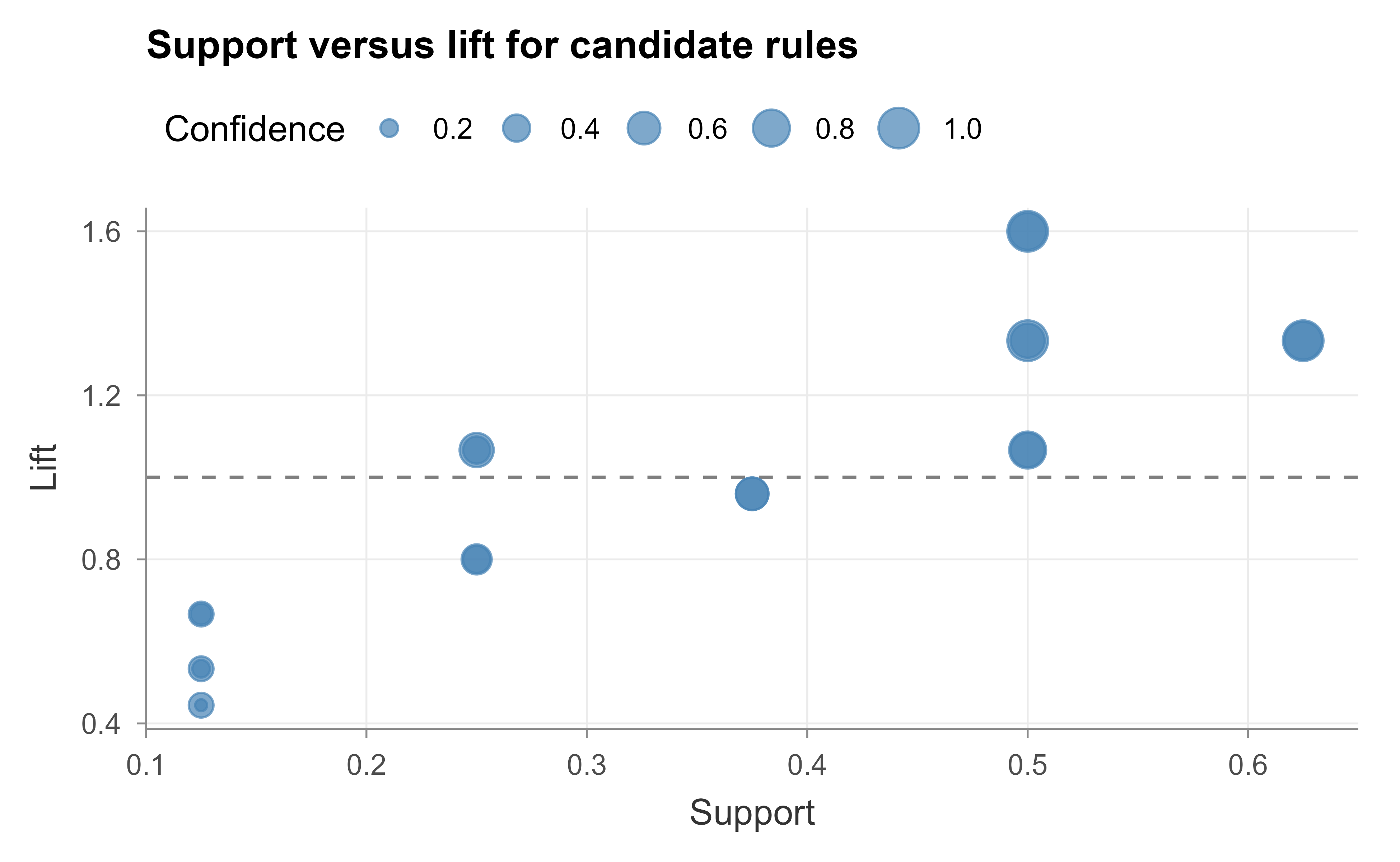
Figure 33.1 visualizes the support-versus-lift trade-off for all candidate rules of the form (single item) $\Rightarrow$ (single item), making concrete why we filter on both axes rather than confidence alone.

Show code

pairs <- expand.grid(X = items, Y = items, stringsAsFactors = FALSE)
pairs <- pairs[pairs$X != pairs$Y, ]
m <- do.call(rbind, Map(function(x, y) rule_metrics(x, y), pairs$X, pairs$Y))
df <- cbind(pairs, m)

library(ggplot2)
ggplot(df, aes(x = support, y = lift)) +
  geom_hline(yintercept = 1, linetype = "dashed", colour = "grey50") +
  geom_point(aes(size = confidence), alpha = 0.7, colour = "steelblue") +
  scale_size_continuous(range = c(1.5, 6)) +
  labs(x = "Support", y = "Lift", size = "Confidence",
       title = "Support versus lift for candidate rules") +
  theme_book()

Figure 33.1: Every single-item to single-item rule, plotted by support and lift. The dashed line at lift = 1 is the independence baseline: points above it are positive associations, points below it are negative. A rule needs both adequate support (to be general) and lift above one (to beat chance).

33.7.2 The Standard Workflow with arules

In practice nobody hand-codes Apriori. The arules package implements both Apriori and Eclat with efficient C backends, and the companion arulesViz package draws the diagnostic plots. The code below mines the Groceries data (9835 real transactions over 169 product categories), the canonical teaching dataset for this topic. It is shown for reference and not executed here.

Show code

library(arules)
library(arulesViz)

data("Groceries")          # 9835 transactions, 169 items, class "transactions"
summary(Groceries)         # density, most frequent items, basket-size distribution
itemFrequencyPlot(Groceries, topN = 15, type = "absolute")

# Mine frequent rules: at least 0.1% support and 50% confidence.
rules <- apriori(
  Groceries,
  parameter = list(supp = 0.001, conf = 0.5, target = "rules")
)

# Rank by lift and inspect the strongest, most informative rules.
rules <- sort(rules, by = "lift", decreasing = TRUE)
inspect(head(rules, 10))

# Add and view all interest measures from this chapter.
quality(rules) <- cbind(
  quality(rules),
  leverage   = interestMeasure(rules, "leverage",   Groceries),
  conviction = interestMeasure(rules, "conviction", Groceries)
)

# Remove redundant rules, then target a specific consequent.
rules <- rules[!is.redundant(rules)]
whole_milk <- subset(rules, subset = rhs %in% "whole milk" & lift > 2)
inspect(head(sort(whole_milk, by = "confidence"), 5))

# FP-growth-style fast itemset mining via Eclat, plus a scatter plot.
freq_sets <- eclat(Groceries, parameter = list(supp = 0.01, maxlen = 4))
plot(rules, method = "scatterplot", measure = c("support", "confidence"),
     shading = "lift")

The workflow generalizes to that data: set thresholds, mine rules, rank by lift, strip redundant rules, and inspect those whose consequent you care about. The apriori call here would return on the order of several hundred rules, of which only a handful survive a serious lift and redundancy filter.

33.8 Connections and Extensions

Association rule mining sits at the unsupervised end of the spectrum with clustering (Chapter 23) and dimension reduction (Chapter 27), but it has relatives across the supervised line as well. The conditional probabilities it estimates are the same objects a naive Bayes classifier (Chapter 18) manipulates, and “class association rules,” whose consequent is restricted to a class label, are a bridge to associative classification. Frequent-itemset structure also underlies certain feature-construction schemes and recommender systems, where co-occurrence counts seed collaborative filtering.

Several extensions matter in practice. Sequential pattern mining adds order and time, asking not just which items co-occur but in what sequence (the GSP and PrefixSpan algorithms). Multi-level and generalized rules exploit an item taxonomy, mining at the level of product categories before drilling into specific products, which softens the rare-item problem. Quantitative association rules handle numeric attributes by discretizing them into ranges. And statistically sound variants attach formal significance tests with multiple-comparison correction to each rule, directly addressing the spurious-pattern hazard. Across all of these, the two questions and the central principle are unchanged: find what occurs together often enough to matter, then keep only the directional patterns that beat chance, all made tractable by the anti-monotonicity of support.

Takeaways

Association rule mining searches for “if this then that” co-occurrence patterns in unlabeled transaction data. Support measures how general a pattern is and confidence how reliable, but confidence is blind to the consequent’s base rate, so always read lift (departure from independence), and consult leverage (absolute effect) and conviction (directional violation rate) alongside it. The Apriori principle, that support is anti-monotone so every superset of an infrequent set is infrequent, is what makes the otherwise $2^d$-sized search feasible; Apriori realizes it with level-wise candidate generation and FP-growth realizes the same goal with a compressed tree and no candidates. Treat every mined rule as a hypothesis generated by a massive multiple-comparison search: validate it, never confuse it with causation, and rank by lift rather than confidence.

# Association Rule Mining {#sec-association-rules} ```{r} #| include: false source("_common.R") ``` Picture the checkout logs of a grocery store. Every receipt is a small, unordered set of items: someone bought bread, butter, and jam; someone else bought beer, chips, and diapers. There is no outcome variable, no label, no "right answer" to predict. Yet hidden in these millions of baskets are regularities a manager would love to know: people who buy bread and butter tend to buy jam, and that pattern repeats far more often than chance would allow. Association rule mining is the set of techniques for surfacing exactly these "if this, then that" patterns from large collections of co-occurrences, without anyone telling the algorithm in advance what to look for. Because there is no target variable guiding the search, association rule mining belongs to unsupervised learning (@sec-intro-unsupervised), alongside cluster analysis (@sec-cluster) and dimension reduction (@sec-dimension-reduction). The difference is what we are looking for. Clustering groups *observations* (whole baskets) that resemble one another; association mining instead looks for *co-occurrence among the items themselves*, and reports its findings as human-readable rules rather than as a partition. The classic setting is market-basket analysis, but the same machinery describes which web pages are viewed together, which symptoms co-occur in patient records, and which words appear in the same document. The whole subject rests on two questions we will make precise. First, which sets of items occur together often enough to be worth our attention (frequent itemset mining)? Second, among those frequent sets, which directional rules are both reliable and genuinely informative (rule generation and evaluation)? The reason the field exists as a separate discipline, rather than being a footnote to probability, is that the first question is computationally brutal: with $d$ distinct items there are $2^d - 1$ possible itemsets, and naive enumeration is hopeless. The central algorithmic insight, the Apriori principle, is what makes the search tractable. ::: {.callout-important title="Key idea"} Association rule mining does not test a hypothesis you brought to the data. It searches an enormous space of possible patterns and reports the ones that pass thresholds you set. The thresholds (and the interest measure you choose) are the modeling decisions, and a rule with stellar confidence can still be worthless. We will see exactly why, and what to use instead. ::: ## The Market-Basket Model We begin by fixing notation. Let $I = \{i_1, i_2, \dots, i_d\}$ be the set of all $d$ available **items** (the store's catalog). A **transaction** $t$ is a subset of items, $t \subseteq I$, and the **database** is a collection of $n$ transactions $T = \{t_1, \dots, t_n\}$. An **itemset** $X$ is any subset of $I$; a $k$-itemset is one with $|X| = k$. It is convenient to view the database as an $n \times d$ binary matrix, with rows indexing transactions and columns indexing items, where entry $(j, m)$ is $1$ if transaction $t_j$ contains item $i_m$ and $0$ otherwise. This makes the connection to ordinary tabular data explicit: market-basket data is just very wide, very sparse binary data, and the quantity that holds our pattern of zeros and ones is what every measure below counts. The **support count** of an itemset $X$ is the number of transactions that contain it, $$ \sigma(X) = \bigl| \{ t_j \in T : X \subseteq t_j \} \bigr|, $$ {#eq-association-rules-supportcount} and its **support** is the fraction of transactions containing it, $$ \operatorname{supp}(X) = \frac{\sigma(X)}{n} = \widehat{\Pr}(X \subseteq t). $$ {#eq-association-rules-support} The second equality is the bridge to probability and is worth stating plainly: if we draw a transaction at random from the database, $\operatorname{supp}(X)$ is the empirical probability that it contains all of $X$. Every interest measure in this chapter is ultimately a function of such empirical probabilities. An **association rule** is an implication of the form $X \Rightarrow Y$, where $X$ and $Y$ are itemsets with $X \cap Y = \varnothing$. We call $X$ the **antecedent** (or left-hand side) and $Y$ the **consequent** (right-hand side). The rule is *not* a logical implication and *not* a causal claim; it is a statistical statement that transactions containing $X$ tend also to contain $Y$. Making "tend to" precise is the job of the next section. ## Interest Measures A rule $X \Rightarrow Y$ has two components we want to quantify: how often the pattern occurs at all, and how strongly the antecedent predicts the consequent. The first is support; the second is captured by a family of measures, each with a probabilistic reading and each with a characteristic blind spot. ### Support and Confidence The **support** of a rule is the support of the union of its two sides, $$ \operatorname{supp}(X \Rightarrow Y) = \operatorname{supp}(X \cup Y) = \widehat{\Pr}(X \cup Y), $$ {#eq-association-rules-rulesupport} the empirical probability that a transaction contains every item in both $X$ and $Y$. Support measures how *general* a rule is: a rule with tiny support describes a corner case that may be a statistical fluke and is rarely actionable. The **confidence** of a rule is the conditional empirical probability of the consequent given the antecedent, $$ \operatorname{conf}(X \Rightarrow Y) = \frac{\operatorname{supp}(X \cup Y)}{\operatorname{supp}(X)} = \widehat{\Pr}(Y \mid X). $$ {#eq-association-rules-confidence} Confidence measures how *reliable* the rule is: among transactions that contain $X$, what fraction also contain $Y$. A confidence of $0.9$ for $\{\text{bread}, \text{butter}\} \Rightarrow \{\text{jam}\}$ says that nine of every ten butter-and-bread baskets also held jam. ::: {.callout-note} Confidence is exactly the maximum-likelihood estimate of $\Pr(Y \mid X)$ in the same sense that a sample proportion estimates a probability. This is why association mining is sometimes described as estimating a large collection of conditional probabilities and keeping only the sharp ones. The naive Bayes classifier (@sec-naive-bayes) rests on the same conditional-probability primitives, differing chiefly in that it has a designated label to condition toward. ::: ### Lift, Leverage, and Conviction Confidence has a famous defect: it ignores how common the consequent is on its own. If $90\%$ of *all* baskets contain milk, then a rule "$\Rightarrow$ milk" with confidence $0.9$ tells us nothing, since we could achieve it by predicting milk for everyone. To correct for the baseline frequency of $Y$ we use **lift**, the ratio of the rule's confidence to the unconditional support of the consequent, $$ \operatorname{lift}(X \Rightarrow Y) = \frac{\operatorname{conf}(X \Rightarrow Y)}{\operatorname{supp}(Y)} = \frac{\operatorname{supp}(X \cup Y)}{\operatorname{supp}(X)\,\operatorname{supp}(Y)} = \frac{\widehat{\Pr}(X \cup Y)}{\widehat{\Pr}(X)\,\widehat{\Pr}(Y)}. $$ {#eq-association-rules-lift} The last form makes the interpretation transparent. Lift is the ratio of the joint probability to the product of the marginals, so it compares the observed co-occurrence against what we would expect if $X$ and $Y$ were statistically independent. A value $\operatorname{lift} = 1$ means $X$ and $Y$ are independent (the rule carries no information beyond base rates); $\operatorname{lift} > 1$ means they appear together more than chance predicts (a positive association); and $\operatorname{lift} < 1$ means they appear together less than chance (a negative association). Lift is symmetric in $X$ and $Y$, which is both a virtue (it is a clean dependence measure) and a limitation (it forgets the rule's direction). **Leverage** measures the same departure from independence on an additive rather than multiplicative scale, $$ \operatorname{leverage}(X \Rightarrow Y) = \operatorname{supp}(X \cup Y) - \operatorname{supp}(X)\,\operatorname{supp}(Y). $$ {#eq-association-rules-leverage} Leverage is the number of *extra* co-occurrences (as a fraction of the database) beyond the independence baseline. It is zero under independence and is bounded in $[-0.25, 0.25]$, which gives a sense of absolute effect size that lift lacks: a rule can have huge lift while leverage is negligible if both items are individually rare. **Conviction** addresses confidence's blind spot from the angle of implication failure, $$ \operatorname{conviction}(X \Rightarrow Y) = \frac{1 - \operatorname{supp}(Y)}{1 - \operatorname{conf}(X \Rightarrow Y)} = \frac{\widehat{\Pr}(X)\,\widehat{\Pr}(\lnot Y)}{\widehat{\Pr}(X \cup \lnot Y)}. $$ {#eq-association-rules-conviction} The numerator is the frequency with which $Y$ is absent overall, and the denominator is the frequency with which the rule is "violated" (that is, $X$ present but $Y$ absent), so conviction is high when the rule is rarely broken relative to how often $Y$ is missing in general. Under independence conviction equals $1$; a logically perfect rule (confidence $1$, never violated) sends conviction to $\infty$. Unlike lift, conviction is directional, distinguishing $X \Rightarrow Y$ from $Y \Rightarrow X$, which often matters in practice. | Measure | Formula | Independence value | Direction-aware | |---|---|---|---| | Support | $\widehat{\Pr}(X \cup Y)$ | (frequency) | no | | Confidence | $\widehat{\Pr}(Y \mid X)$ | $\operatorname{supp}(Y)$ | yes | | Lift | $\widehat{\Pr}(X \cup Y) / (\widehat{\Pr}(X)\widehat{\Pr}(Y))$ | $1$ | no | | Leverage | $\widehat{\Pr}(X\cup Y) - \widehat{\Pr}(X)\widehat{\Pr}(Y)$ | $0$ | no | | Conviction | $\widehat{\Pr}(X)\widehat{\Pr}(\lnot Y)/\widehat{\Pr}(X\cup\lnot Y)$ | $1$ | yes | : Interest measures for a rule $X \Rightarrow Y$, their probabilistic form, the value they take when $X$ and $Y$ are independent, and whether they distinguish the rule from its reverse. {#tbl-association-rules-measures} @tbl-association-rules-measures collects these together. No single measure dominates: confidence is interpretable but baseline-blind, lift is a clean dependence score but undirected and unstable for rare items, leverage gives absolute effect size, and conviction restores direction. Mature practice reports several and reads them together. ## The Apriori Principle and Algorithm We now confront the computational obstacle. To find all rules above given support and confidence thresholds, it suffices first to find all **frequent itemsets**, those $X$ with $\operatorname{supp}(X) \ge \operatorname{minsupp}$, and then to generate rules from them (next section). The trouble is that there are $2^d - 1$ candidate itemsets, an astronomically large number for a real catalog. We cannot count support for all of them. The Apriori principle is what saves us. ### Downward Closure: A Derivation The principle is a monotonicity statement about support, and it follows directly from the definition. ::: {.callout-tip title="Apriori principle (downward closure)"} If an itemset is frequent, then every one of its subsets is also frequent. Equivalently, if an itemset is *infrequent*, then every one of its supersets is also infrequent. ::: To prove it, let $X \subseteq Y$ be two itemsets, so $X$ is a subset of $Y$. Any transaction that contains $Y$ must, by definition of subset, contain $X$ as well. Therefore the set of transactions containing $Y$ is a subset of the set of transactions containing $X$, which gives $$ \sigma(Y) \le \sigma(X) \quad\Longrightarrow\quad \operatorname{supp}(Y) \le \operatorname{supp}(X). $$ {#eq-association-rules-antimonotone} In words, support is **anti-monotone**: enlarging an itemset can only keep its support the same or shrink it, never raise it. Now suppose $X$ is infrequent, $\operatorname{supp}(X) < \operatorname{minsupp}$. For any superset $Y \supseteq X$, @eq-association-rules-antimonotone gives $\operatorname{supp}(Y) \le \operatorname{supp}(X) < \operatorname{minsupp}$, so $Y$ is infrequent too. This is the contrapositive of the principle, and it is the engine of pruning: the moment we find an itemset to be infrequent, we may discard *all* of its supersets without ever counting their support. Whole subtrees of the search space vanish at once. ### The Apriori Algorithm The Apriori algorithm [@agrawal1994] turns the principle into a breadth-first, level-wise search. It builds frequent itemsets of size $k$ only from frequent itemsets of size $k-1$, so an itemset is even *considered* (made a candidate) only if all of its immediate subsets already qualified. Let $L_k$ denote the set of frequent $k$-itemsets and $C_k$ the set of candidate $k$-itemsets. The procedure is: 1. **Initialize.** Scan the database once to compute the support of every single item; keep those above $\operatorname{minsupp}$ as $L_1$. 2. **Candidate generation.** From $L_{k-1}$, form candidates $C_k$ by joining pairs of frequent $(k-1)$-itemsets that share their first $k-2$ items (the "join" step). 3. **Prune.** Remove from $C_k$ any candidate that has a $(k-1)$-subset not present in $L_{k-1}$. By downward closure such a candidate cannot be frequent, so we drop it before wasting a database scan on it (the "prune" step). 4. **Count.** Scan the database once to count the support of the surviving candidates in $C_k$; keep those above $\operatorname{minsupp}$ as $L_k$. 5. **Repeat** steps 2 to 4, incrementing $k$, until $L_k$ is empty. The frequent itemsets are $\bigcup_k L_k$. Each level costs one pass over the data, so a database with maximum frequent-itemset size $k_{\max}$ requires about $k_{\max}+1$ passes. The work per pass is dominated by support counting, often implemented with a hash tree so that each transaction is matched against candidates efficiently. In the worst case (a very low threshold on dense data) the candidate set can still explode, but on the sparse, threshold-pruned itemsets typical of retail data Apriori is dramatically faster than brute force. ::: {.callout-warning} Apriori's Achilles heel is candidate generation. When many itemsets clear the support threshold, $C_k$ can become enormous, and each database scan grows expensive. Repeatedly scanning a large database, once per level, is the practical bottleneck that motivated the next algorithm. ::: ## FP-Growth: Mining Without Candidate Generation FP-growth [@han2000] attacks Apriori's two costs (repeated scans and candidate explosion) by compressing the database into a tree and mining that tree directly, never generating candidates at all. The idea proceeds in two passes. The first pass counts single-item supports and discards infrequent items, then fixes an ordering of the remaining frequent items by decreasing support. The second pass reads each transaction, drops its infrequent items, sorts the rest into the fixed order, and inserts the result as a path into a prefix tree called the **FP-tree**. Transactions that share a prefix share the upper portion of their path, and a counter on each node records how many transactions pass through it. Frequent items appearing in many baskets sit near the root and are stored once rather than repeatedly, so the tree is a compressed, lossless summary of all the frequency information needed. A header table links together all nodes for a given item, so the tree can be traversed by item. Mining then works recursively and bottom-up. For each item (starting from the least frequent), the algorithm collects that item's **conditional pattern base**, the set of prefix paths leading to it, weighted by counts, and builds a smaller **conditional FP-tree** from those paths. Frequent itemsets ending in that item are read off by recursing into the conditional tree. Because the patterns are grown by extending known frequent fragments rather than by proposing and testing candidates, FP-growth performs only two database scans total and avoids candidate generation entirely. The price is memory: the FP-tree must fit in RAM, and on dense data where little prefix sharing occurs the tree can be large. In broad strokes, Apriori trades memory for repeated computation while FP-growth trades computation for memory, and the better choice depends on data density and size. ## Rule Generation and Pruning Finding frequent itemsets answers the first question; we still must turn them into rules. The key observation is that a rule's support is fixed once we choose the itemset, so support never has to be recomputed at this stage. For a frequent itemset $Z$, every rule of the form $X \Rightarrow Z \setminus X$ (for nonempty proper subsets $X \subset Z$) has the same support $\operatorname{supp}(Z)$, automatically above $\operatorname{minsupp}$. The only thing left to check is confidence. This sets up a second pruning opportunity that mirrors downward closure. Consider moving an item from the antecedent to the consequent, that is, comparing $X \Rightarrow Z \setminus X$ against a rule with a *smaller* antecedent and *larger* consequent. Because the antecedent shrinks, its support can only grow (by @eq-association-rules-antimonotone applied to the antecedent), and since $\operatorname{conf} = \operatorname{supp}(Z)/\operatorname{supp}(\text{antecedent})$ with a fixed numerator, a larger denominator means smaller confidence. Formally, confidence is anti-monotone with respect to enlarging the consequent: if a rule with consequent $Y$ fails the confidence threshold, then every rule obtained from the same itemset by moving more items into the consequent also fails. We can therefore prune low-confidence rules level by level over consequent size, exactly as Apriori prunes itemsets, generating high-confidence rules without examining every subset split. Once rules clear the confidence threshold, they are typically ranked and filtered by the additional interest measures of @tbl-association-rules-measures, most often lift, and frequently de-duplicated by removing **redundant** rules. A rule is redundant if a more general rule (one with the same or higher confidence and a subset antecedent) already exists, since the extra antecedent items add specificity without predictive gain. ## Pitfalls: Why Confidence Is Not Enough The single most important practical lesson is that high confidence does not imply a useful rule, and the reason is the baseline blindness we flagged earlier. The cleanest illustration is the classic tea-and-coffee example. ::: {.callout-important title="The high-confidence trap"} Suppose $80\%$ of all customers buy coffee, and $25\%$ buy tea. Among tea buyers, $80\%$ also buy coffee. The rule $\{\text{tea}\} \Rightarrow \{\text{coffee}\}$ has confidence $0.80$, which sounds strong. But coffee is bought by $80\%$ of *everyone*, so buying tea does not raise the chance of buying coffee at all. The lift is $0.80 / 0.80 = 1$: tea and coffee are independent, and the rule is worthless despite its high confidence. In fact, if tea buyers bought coffee at $70\%$ (below the $80\%$ base rate), the rule would still have respectable confidence yet a lift of $0.875 < 1$, signaling a *negative* association that confidence alone completely hides. ::: This is why mature practice never ranks by confidence alone. Three further hazards deserve naming. First is **multiple comparisons**: an automated search over millions of candidate rules will, purely by chance, surface some with impressive statistics on any finite database, so apparent patterns demand validation on held-out data or correction for the number of rules examined. This is the same garden-of-forking-paths concern that haunts any large unsupervised search, and it connects to the broader project of interpretable machine learning (@sec-interpretable-machine-learning), where the goal is explanations one can actually trust. Second is the **rare-item problem**: a single global $\operatorname{minsupp}$ either drowns out interesting but infrequent items (set it high) or floods the output with noise (set it low). Third, and most fundamental, **association is not causation**: a rule $X \Rightarrow Y$ describes co-occurrence in a particular population and gives no license to conclude that stocking $X$ will sell more $Y$. The famous "beer and diapers" story, whatever its provenance, is at best a correlation discovered post hoc. ## Demonstration We work through two demonstrations. The first computes support, confidence, lift, leverage, and conviction entirely in base R on a tiny set of baskets, so that every formula above is visible as code. The second shows the standard production workflow with the `arules` package on the well-known `Groceries` dataset; it is displayed but not executed here, since `arules` may not be installed. ### From Scratch in Base R We hand-build a small grocery database as a binary transaction matrix and implement @eq-association-rules-support through @eq-association-rules-conviction directly. This is the runnable, verified portion. ```{r} #| label: association-rules-scratch # A tiny transaction database: rows = baskets, cols = items, 1 = present. items <- c("bread", "butter", "jam", "milk", "beer") baskets <- rbind( c(1, 1, 1, 0, 0), # bread, butter, jam c(1, 1, 1, 1, 0), # bread, butter, jam, milk c(1, 1, 0, 1, 0), # bread, butter, milk c(1, 0, 0, 1, 0), # bread, milk c(0, 0, 0, 1, 1), # milk, beer c(1, 1, 1, 0, 0), # bread, butter, jam c(0, 0, 0, 0, 1), # beer c(1, 1, 1, 1, 1) # everything ) colnames(baskets) <- items n <- nrow(baskets) # supp(X): fraction of baskets containing every item in the set X. supp <- function(X, data = baskets) { cols <- data[, X, drop = FALSE] mean(rowSums(cols) == length(X)) } # All five interest measures for a rule X => Y. rule_metrics <- function(X, Y, data = baskets) { sXY <- supp(c(X, Y), data); sX <- supp(X, data); sY <- supp(Y, data) conf <- sXY / sX data.frame( support = sXY, confidence = conf, lift = conf / sY, leverage = sXY - sX * sY, conviction = if (conf < 1) (1 - sY) / (1 - conf) else Inf ) } # Rule 1: {bread, butter} => {jam} (expect strong, informative) # Rule 2: {beer} => {milk} (expect weak / near-independent) r1 <- rule_metrics(c("bread", "butter"), "jam") r2 <- rule_metrics("beer", "milk") out <- rbind(`{bread,butter} => {jam}` = r1, `{beer} => {milk}` = r2) round(out, 3) ``` The first rule has high confidence *and* lift above one, so bread-and-butter buyers really do buy jam more than the base rate predicts. Reading the second rule shows the pitfall in miniature: even where confidence is non-trivial, the lift reveals whether the association beats chance. We can also reproduce the Apriori downward-closure pruning by hand, confirming that no superset of an infrequent itemset survives. ```{r} #| label: association-rules-apriori # Brute-force frequent itemsets, then verify downward closure. minsupp <- 0.30 all_sets <- unlist( lapply(1:length(items), function(k) combn(items, k, simplify = FALSE)), recursive = FALSE ) supports <- vapply(all_sets, supp, numeric(1)) frequent <- all_sets[supports >= minsupp] # Downward closure: every subset of a frequent set is also frequent. freq_keys <- vapply(frequent, function(s) paste(sort(s), collapse = ","), "") closure_ok <- all(vapply(frequent, function(s) { if (length(s) == 1) return(TRUE) subs <- combn(s, length(s) - 1, simplify = FALSE) all(vapply(subs, function(z) paste(sort(z), collapse = ",") %in% freq_keys, TRUE)) }, TRUE)) cat("Number of frequent itemsets (supp >=", minsupp, "):", length(frequent), "\n") cat("Downward closure holds for all frequent itemsets:", closure_ok, "\n") ``` @fig-association-rules-lift visualizes the support-versus-lift trade-off for all candidate rules of the form (single item) $\Rightarrow$ (single item), making concrete why we filter on both axes rather than confidence alone. ```{r} #| label: fig-association-rules-lift #| fig-cap: "Every single-item to single-item rule, plotted by support and lift. The dashed line at lift = 1 is the independence baseline: points above it are positive associations, points below it are negative. A rule needs both adequate support (to be general) and lift above one (to beat chance)." pairs <- expand.grid(X = items, Y = items, stringsAsFactors = FALSE) pairs <- pairs[pairs$X != pairs$Y, ] m <- do.call(rbind, Map(function(x, y) rule_metrics(x, y), pairs$X, pairs$Y)) df <- cbind(pairs, m) library(ggplot2) ggplot(df, aes(x = support, y = lift)) + geom_hline(yintercept = 1, linetype = "dashed", colour = "grey50") + geom_point(aes(size = confidence), alpha = 0.7, colour = "steelblue") + scale_size_continuous(range = c(1.5, 6)) + labs(x = "Support", y = "Lift", size = "Confidence", title = "Support versus lift for candidate rules") + theme_book() ``` ### The Standard Workflow with arules In practice nobody hand-codes Apriori. The `arules` package implements both Apriori and Eclat with efficient C backends, and the companion `arulesViz` package draws the diagnostic plots. The code below mines the `Groceries` data (9835 real transactions over 169 product categories), the canonical teaching dataset for this topic. It is shown for reference and not executed here. ```{r} #| label: association-rules-arules #| eval: false library(arules) library(arulesViz) data("Groceries") # 9835 transactions, 169 items, class "transactions" summary(Groceries) # density, most frequent items, basket-size distribution itemFrequencyPlot(Groceries, topN = 15, type = "absolute") # Mine frequent rules: at least 0.1% support and 50% confidence. rules <- apriori( Groceries, parameter = list(supp = 0.001, conf = 0.5, target = "rules") ) # Rank by lift and inspect the strongest, most informative rules. rules <- sort(rules, by = "lift", decreasing = TRUE) inspect(head(rules, 10)) # Add and view all interest measures from this chapter. quality(rules) <- cbind( quality(rules), leverage = interestMeasure(rules, "leverage", Groceries), conviction = interestMeasure(rules, "conviction", Groceries) ) # Remove redundant rules, then target a specific consequent. rules <- rules[!is.redundant(rules)] whole_milk <- subset(rules, subset = rhs %in% "whole milk" & lift > 2) inspect(head(sort(whole_milk, by = "confidence"), 5)) # FP-growth-style fast itemset mining via Eclat, plus a scatter plot. freq_sets <- eclat(Groceries, parameter = list(supp = 0.01, maxlen = 4)) plot(rules, method = "scatterplot", measure = c("support", "confidence"), shading = "lift") ``` The workflow generalizes to that data: set thresholds, mine rules, rank by lift, strip redundant rules, and inspect those whose consequent you care about. The `apriori` call here would return on the order of several hundred rules, of which only a handful survive a serious lift and redundancy filter. ## Connections and Extensions Association rule mining sits at the unsupervised end of the spectrum with clustering (@sec-cluster) and dimension reduction (@sec-dimension-reduction), but it has relatives across the supervised line as well. The conditional probabilities it estimates are the same objects a naive Bayes classifier (@sec-naive-bayes) manipulates, and "class association rules," whose consequent is restricted to a class label, are a bridge to associative classification. Frequent-itemset structure also underlies certain feature-construction schemes and recommender systems, where co-occurrence counts seed collaborative filtering. Several extensions matter in practice. **Sequential pattern mining** adds order and time, asking not just which items co-occur but in what sequence (the GSP and PrefixSpan algorithms). **Multi-level and generalized rules** exploit an item taxonomy, mining at the level of product categories before drilling into specific products, which softens the rare-item problem. **Quantitative association rules** handle numeric attributes by discretizing them into ranges. And **statistically sound** variants attach formal significance tests with multiple-comparison correction to each rule, directly addressing the spurious-pattern hazard. Across all of these, the two questions and the central principle are unchanged: find what occurs together often enough to matter, then keep only the directional patterns that beat chance, all made tractable by the anti-monotonicity of support. ::: {.callout-important title="Takeaways"} Association rule mining searches for "if this then that" co-occurrence patterns in unlabeled transaction data. Support measures how general a pattern is and confidence how reliable, but confidence is blind to the consequent's base rate, so always read lift (departure from independence), and consult leverage (absolute effect) and conviction (directional violation rate) alongside it. The Apriori principle, that support is anti-monotone so every superset of an infrequent set is infrequent, is what makes the otherwise $2^d$-sized search feasible; Apriori realizes it with level-wise candidate generation and FP-growth realizes the same goal with a compressed tree and no candidates. Treat every mined rule as a hypothesis generated by a massive multiple-comparison search: validate it, never confuse it with causation, and rank by lift rather than confidence. :::