Imagine you have a folder of ten thousand photographs of faces and you want a computer to produce a brand new face that no one has ever seen, yet looks completely real. A classifier cannot do this. A classifier reads a photo and returns a label such as “smiling” or “not smiling”. It never has to understand what makes a face a face. To invent a new one, the computer needs a model of what faces look like in general, not just a rule for telling two kinds apart. That distinction, between a model that labels data and a model that can produce data, is the subject of this chapter.
Most of this book studies discriminative models. A discriminative model learns \(p(y \mid x)\) directly: given an input \(x\), it returns a label or a number. A generative model instead learns the data distribution itself, either the joint \(p(x, y)\) or the marginal \(p(x)\). Once you have a model of \(p(x)\), you can do more than classify. You can draw new samples that look like the training data, score how likely a point is, fill in missing parts of an input, and compress data into a compact code.
Intuition
A discriminative model learns where to draw the line between categories. A generative model learns the whole landscape the data live on, so it can walk around and produce new points anywhere on that landscape.
This chapter covers three families that dominate modern generative modeling: variational autoencoders (VAEs), generative adversarial networks (GANs), and diffusion models. For each one you will see the intuition first, then the math that makes it precise, then a sketch of the code, and finally what the result means. The three families reach the same goal, a model you can sample from, by very different routes, and the closing comparison lays out the trade-offs side by side. The runnable demonstration near the end uses base R and ggplot2 only, so every number in it reproduces without a deep learning backend.1
42.1 Generative versus Discriminative
Before meeting the three model families, it is worth pinning down precisely what “generative” means and why it is a different job from the classification and regression that occupy much of this book. The cleanest way in is to write the joint distribution two ways:
A discriminative model targets the first factor \(p(y \mid x)\) and ignores \(p(x)\). Logistic regression, random forests, and the neural network classifiers from earlier chapters all sit here. They tend to predict well because they spend all of their capacity on the boundary between classes.
A generative model targets \(p(x \mid y)\) and \(p(y)\), or just \(p(x)\) when there are no labels. Classification then comes from Bayes rule,
Naive Bayes (Chapter 18) and Gaussian discriminant analysis (Chapter 20) are classic examples. Modeling \(p(x)\) is harder than modeling a boundary, because the model has to account for everything in the data, not just the part that separates classes. So why pay that price? Classification is only one of several payoffs. A model of \(p(x)\) lets you:
sample new data, for example images, audio, or molecules,
detect outliers as points with low \(p(x)\) (Chapter 87),
impute missing features,
learn a useful low dimensional representation,
augment a small training set with synthetic examples.
Note
None of the three families below require the labels \(y\). They learn the shape of \(p(x)\) from inputs alone, which is why they are usually trained on unlabeled data, of which the world has far more than labeled data.
The three families take different routes to a model you can sample from. We start with the one closest to ideas already in this book, the autoencoder.
42.2 Variational Autoencoders
The first family stays closest to familiar territory. A variational autoencoder (VAE) is a latent variable model: it assumes each observed point \(x\) is generated from an unobserved, low dimensional code \(z\) that we never see directly. The generative story is
\[
z \sim p(z) = \mathcal{N}(0, I), \qquad x \sim p_\theta(x \mid z),
\]
so the marginal likelihood of a data point integrates over the latent variable,
Here \(z\) is the latent code, a short vector that captures the essence of \(x\) (say, a handful of numbers summarizing a face), and \(p_\theta(x \mid z)\) is the decoder, the network with parameters \(\theta\) that turns a code back into a data point.
This connects to the autoencoders chapter (Chapter 41). A plain autoencoder maps \(x\) to a code and back with no probabilistic meaning. A VAE keeps the encoder and decoder shape but makes both stochastic, which lets us sample new \(x\) by drawing \(z \sim \mathcal{N}(0, I)\) and passing it through the decoder.
Key idea
A plain autoencoder compresses and reconstructs. A VAE turns that same architecture into a generator by insisting the codes follow a known distribution, the standard normal, so you can sample a fresh code and decode it into a new, plausible \(x\).
42.2.1 The problem with the integral
There is a snag. To train the model we would like to maximize \(p_\theta(x)\), but the integral over \(z\) has no closed form for a neural network decoder, and the posterior \(p_\theta(z \mid x) = p_\theta(x \mid z)\, p(z) / p_\theta(x)\) (which codes are likely to have produced a given \(x\)) is equally hard. The VAE works around both by introducing a second network, an encoder \(q_\phi(z \mid x)\), that approximates the true posterior. The encoder outputs a mean and a variance,
Because we cannot maximize \(\log p_\theta(x)\) directly, we maximize a quantity that is guaranteed to sit just below it and is computable. Start from the log marginal likelihood and insert \(q_\phi\):
It is worth deriving the same bound a second way, by an exact identity rather than an inequality, because the algebra reveals precisely what is lost. For any \(q_\phi(z \mid x)\) with the same support as the posterior, multiply and divide inside the log and split the expectation:
where the first line uses that \(\log p_\theta(x)\) does not depend on \(z\), the second uses \(p_\theta(x) = p_\theta(x, z) / p_\theta(z \mid x)\), and the last line recognizes \(\mathbb{E}_{q_\phi}[\log p_\theta(x, z) - \log q_\phi] = \mathcal{L}\) once \(p_\theta(x, z) = p_\theta(x \mid z)\, p(z)\) is expanded. Equation Equation 42.1 is exact: the log evidence equals the ELBO plus a non negative KL term, so the ELBO is a lower bound, and the inequality is tight exactly when \(q_\phi\) equals the true posterior.
The gap between \(\log p_\theta(x)\) and the ELBO is exactly \(D_{\mathrm{KL}}(q_\phi(z \mid x)\,\|\,p_\theta(z \mid x))\), which is non negative,2 so maximizing \(\mathcal{L}\) does two good things at once: it pushes the bound up and it makes the approximate posterior close to the true one.
Read the two terms as a loss. The first term is a reconstruction term: it rewards a decoder that assigns high probability to the actual \(x\) given its code. The second term is a Kullback Leibler penalty that pulls the encoded distribution toward the prior \(\mathcal{N}(0, I)\). The KL term acts as a regularizer. Without it the encoder could place every input in its own tiny region of latent space, which would reconstruct well but leave gaps that decode to nothing. The penalty keeps the latent space packed near the prior so that random draws decode into plausible samples.
Intuition
Picture the reconstruction term as “remember the data” and the KL term as “stay tidy”. Pull only on the first and the model memorizes inputs into scattered, unusable codes. Pull only on the second and every input collapses to the same blurry average. The ELBO balances the two.
When both \(q_\phi(z \mid x)\) and \(p(z)\) are Gaussian the KL term has a closed form, so there is nothing to estimate by sampling. For a \(d\) dimensional diagonal Gaussian,
The closed form is worth deriving once, because it explains why each term has the sign it does. The KL divergence between two univariate Gaussians \(\mathcal{N}(\mu_1, \sigma_1^2)\) and \(\mathcal{N}(\mu_2, \sigma_2^2)\) is
Under \(q\) we have \(\mathbb{E}_q[(z - \mu_1)^2] = \sigma_1^2\) and \(\mathbb{E}_q[(z - \mu_2)^2] = \sigma_1^2 + (\mu_1 - \mu_2)^2\), so the expectation collapses to
Setting the prior to the standard normal, \(\mu_2 = 0\) and \(\sigma_2 = 1\), and summing over the \(d\) independent coordinates of the diagonal posterior gives Equation 42.2. The quadratic terms \(\mu_j^2\) and \(\sigma_j^2\) penalize codes that drift from the origin or spread too wide, while the \(-\log \sigma_j^2\) term forbids the variance from collapsing to zero, which would make the posterior a point mass and the latent space unusable for sampling.
Posterior collapse
A characteristic VAE failure is posterior collapse, where for some latent coordinates the encoder ignores the input and returns \(q_\phi(z_j \mid x) \approx p(z_j) = \mathcal{N}(0, 1)\), driving the KL term in Equation 42.2 to zero. The decoder then learns to reconstruct without using those coordinates, so they carry no information. This happens most often when the decoder is powerful enough to model \(x\) on its own (for example an autoregressive decoder) and early in training when the reconstruction term is weak. Standard remedies are KL annealing (warm up the KL weight from zero), free bits (clamp each coordinate’s KL at a small floor \(\lambda\) so the optimizer stops shrinking it once it is informative enough), or the \(\beta\)-VAE weighting below.
42.2.3 Amortized inference and the \(\beta\)-VAE
The encoder \(q_\phi(z \mid x)\) deserves a second look. Classical variational inference fits a separate set of variational parameters \((\mu_i, \sigma_i)\) for every data point \(x_i\), solving an optimization per example. The VAE instead trains a single network that maps any \(x\) to its \((\mu_\phi(x), \sigma_\phi(x))\), sharing parameters across the whole dataset. This is amortized inference: the cost of inference is amortized over the dataset by paying once to train the encoder, after which a new point’s approximate posterior is a single forward pass. The price is the amortization gap, the extra slack between the ELBO achieved by the shared encoder and the best ELBO a per example optimizer could reach. Together with the approximation gap from \(q_\phi\) being Gaussian rather than the true posterior, this is why the ELBO can sit well below \(\log p_\theta(x)\).
The full training objective is the ELBO averaged over the data, and the gradient with respect to \(\theta\) and \(\phi\) is estimated by drawing a minibatch and one reparameterized \(\epsilon\) per example. A widely used generalization scales the KL term by a constant \(\beta\),
With \(\beta = 1\) this is the exact ELBO. Setting \(\beta > 1\) presses the aggregated posterior harder toward the factorized prior, which tends to produce more disentangled latent coordinates at the cost of reconstruction fidelity, while \(\beta < 1\) favors sharper reconstructions and risks the scattered, gap riddled latent space the KL term is meant to prevent. The reconstruction term has its own implicit weight: with a Gaussian decoder of fixed variance \(\sigma_x^2\), the negative log likelihood is \(\|x - \hat x\|^2 / (2\sigma_x^2)\) up to a constant, so \(\sigma_x^2\) acts as an inverse weight on reconstruction relative to the KL term. This is why a plain mean squared error decoder with no explicit variance implicitly fixes a particular trade-off.
42.2.4 The reparameterization trick
To train with gradient descent we need gradients of \(\mathcal{L}\) with respect to the encoder parameters \(\phi\). The trouble is that the expectation is taken over a distribution that depends on \(\phi\), so we cannot just sample \(z\) and backpropagate through the sampling step. The reparameterization trick rewrites the sample as a deterministic function of \(\phi\) plus external noise,
where \(\odot\) is elementwise multiplication. Now the randomness lives in \(\epsilon\), which does not depend on \(\phi\), and the path from \(\phi\) to \(z\) is differentiable. The Monte Carlo estimate of the ELBO using one or a few draws of \(\epsilon\) then has a well defined gradient.
To see precisely why this matters, compare two ways of differentiating an expectation \(\mathbb{E}_{q_\phi(z)}[f(z)]\) whose distribution depends on \(\phi\). The score function or REINFORCE estimator uses the identity \(\nabla_\phi q_\phi = q_\phi\, \nabla_\phi \log q_\phi\) to write
which is unbiased and needs only \(\log q_\phi\), not a differentiable \(f\), but is notoriously high variance because \(f(z)\) multiplies the score with no cancellation. The reparameterization estimator instead pushes the parameter inside a deterministic map \(z = g_\phi(\epsilon)\) with \(\epsilon \sim p(\epsilon)\) fixed, giving
The Jacobian \(\nabla_\phi g_\phi\) couples the gradient of \(f\) directly to the parameter, so the estimator exploits the smoothness of the decoder and typically has far lower variance, often by orders of magnitude. The cost is that it requires \(f\) (here the integrand of the ELBO) to be differentiable in \(z\), which holds for continuous data and a Gaussian \(q_\phi\) but fails for discrete \(z\), where one falls back on the score function estimator or a continuous relaxation such as the Gumbel-Softmax.
Key idea
You cannot differentiate through “draw a random sample”, but you can differentiate through “scale and shift a fixed random sample”. The reparameterization trick is exactly that move, and it is what makes the VAE trainable by ordinary backpropagation.
The next block sketches a VAE in Keras. It is shown for reference and is marked eval = FALSE because it needs the Keras/TensorFlow backend, which is not available in this build.
Show code
library(keras)latent_dim<-2# Encoder outputs mean and log variance of q(z | x)encoder_in<-layer_input(shape =784)h<-encoder_in%>%layer_dense(256, activation ="relu")z_mean<-h%>%layer_dense(latent_dim)z_log_var<-h%>%layer_dense(latent_dim)# Reparameterization: z = mean + exp(log_var / 2) * epsilonsampling<-function(args){z_mean<-args[[1]]z_log_var<-args[[2]]eps<-k_random_normal(shape =k_shape(z_mean))z_mean+k_exp(0.5*z_log_var)*eps}z<-list(z_mean, z_log_var)%>%layer_lambda(sampling)# Decoder maps z back to xdecoder<-keras_model_sequential()%>%layer_dense(256, activation ="relu", input_shape =latent_dim)%>%layer_dense(784, activation ="sigmoid")x_decoded<-decoder(z)vae<-keras_model(encoder_in, x_decoded)# Loss = reconstruction + KL regularizerrecon<-784*loss_binary_crossentropy(encoder_in, x_decoded)kl<--0.5*k_sum(1+z_log_var-k_square(z_mean)-k_exp(z_log_var), axis =-1L)vae$add_loss(k_mean(recon+kl))vae%>%compile(optimizer ="adam")
42.3 Generative Adversarial Networks
The VAE works hard to keep an explicit, if approximate, handle on the likelihood. A generative adversarial network (GAN) throws that away and asks a different question: instead of “how probable is this data point?”, it asks “can anyone tell my fakes from the real thing?” Think of an art forger and a detective. The forger (the generator) paints fakes; the detective (the discriminator) tries to spot them. Each makes the other better. When the forger finally wins, the fakes are indistinguishable from genuine work.
Concretely, two networks compete. A generator \(G\) maps noise \(z \sim p(z)\) to a fake sample \(G(z)\). A discriminator \(D\) takes a sample and outputs the probability that it is real. Training is a minimax game,
The discriminator wants to push \(D(x)\) toward one on real data and toward zero on fakes. The generator wants the opposite, to make \(D(G(z))\) close to one. The \(\min_G \max_D\) notation reads literally: the inner \(\max_D\) trains the best detective it can, and the outer \(\min_G\) trains the forger to defeat that best detective.
Note
A GAN never writes down or evaluates \(p(x)\). It is an implicit generative model: it can hand you samples but cannot tell you how likely any particular point is. That is the price of skipping the likelihood.
42.3.1 The optimal discriminator
It helps to ask what the perfect detective would do, holding the forger fixed. Fix the generator, so the distribution of fakes \(p_g\) is fixed. Write the value function as a single integral over \(x\),
For each \(x\) the integrand has the form \(a \log d + b \log(1 - d)\), which is maximized at \(d = a / (a + b)\). The optimal discriminator is therefore the density ratio
The collecting of terms is short enough to show. Write \(m = \tfrac12(p_{\mathrm{data}} + p_g)\) for the mixture. Substituting \(D^* = p_{\mathrm{data}} / (2m)\) and \(1 - D^* = p_g / (2m)\) gives
using \(D_{\mathrm{JS}}(p \| q) = \tfrac12 D_{\mathrm{KL}}(p \| m) + \tfrac12 D_{\mathrm{KL}}(q \| m)\) in the last line. This is Equation 42.4. Because \(D_{\mathrm{JS}} \ge 0\) with equality iff \(p_g = p_{\mathrm{data}}\), the outer minimization over \(G\) drives \(p_g\) to the data distribution and the value to its floor \(-\log 4\).
where \(D_{\mathrm{JS}}\) is the Jensen Shannon divergence, a symmetric measure of how far two distributions are apart.3 Since the JS divergence is zero only when \(p_g = p_{\mathrm{data}}\), the generator that wins the game matches the data distribution exactly, with the value reaching its minimum of \(-\log 4\).
Key idea
Underneath the forger-versus-detective story, the GAN is secretly minimizing a divergence between the fake and real distributions. The adversarial game is just a clever, sample-only way to estimate and descend that divergence without ever computing a density.
The demonstration below evaluates \(D^*(x)\) for two Gaussians so the density ratio result is visible as a concrete curve.
42.3.2 Mode collapse and instability
The clean theory above assumes both networks are trained to optimality at each step, which never happens in practice. Two failures are common, and knowing their names is half of diagnosing a misbehaving GAN.
The first is mode collapse: the generator discovers a few outputs that reliably fool the current discriminator and produces only those, ignoring whole regions of the data. The samples look fine one at a time but lack variety, like a forger who only knows how to paint one convincing painting.
The second is training instability: the two networks chase a moving target. If the discriminator gets too strong, the term \(\log(1 - D(G(z)))\) saturates and the generator gradient vanishes, so the forger stops learning precisely when it is losing badly. A common fix is to have the generator maximize \(\log D(G(z))\) instead, which gives stronger gradients early in training. Balancing the two networks, tuning learning rates, and choosing alternative losses such as the Wasserstein objective are all standard parts of getting a GAN to converge.
The saturation is easy to make precise. Let \(u = D(G(z))\) be the discriminator’s probability that a fake is real, small early in training when fakes are obvious. The original generator loss \(\log(1 - u)\) has derivative \(-1/(1 - u)\), which is near \(-1\) when \(u \approx 0\): a tiny, nearly constant gradient exactly when the generator most needs a push. The non saturating surrogate maximizes \(\log u\), whose derivative \(1/u\) blows up as \(u \to 0\), supplying a large gradient when the fakes are poor. Both losses share the same fixed point but have opposite gradient behavior in the regime that matters early on, which is why the non saturating form is the practical default.
42.3.3 Why JS divergence is a brittle objective
The JS divergence result Equation 42.4 is elegant but also diagnoses the deeper instability. When \(p_{\mathrm{data}}\) and \(p_g\) live on low dimensional manifolds in a high dimensional space, as natural images do, their supports are almost surely disjoint or overlap on a set of measure zero early in training. On disjoint supports a perfect discriminator exists, \(D_{\mathrm{JS}}\) is pinned at its maximum \(\log 2\) regardless of how far apart the two distributions are, and its gradient with respect to the generator is zero almost everywhere. The generator receives no signal about which direction would move \(p_g\) toward \(p_{\mathrm{data}}\). This is the manifold view of why a too strong discriminator kills learning.
The Wasserstein GAN replaces JS with the earth mover (Wasserstein-1) distance, which by Kantorovich-Rubinstein duality equals
where the supremum is over all 1-Lipschitz functions \(f\). Unlike JS, \(W\) varies smoothly with the distance between \(p_g\) and \(p_{\mathrm{data}}\) even when their supports do not overlap, so it provides a usable gradient everywhere. In practice \(f\) (now called a critic, with no sigmoid and a real valued output) is constrained to be Lipschitz by weight clipping or, more reliably, a gradient penalty that pushes \(\|\nabla_x f\|\) toward one. The critic loss in Equation 42.5 also tracks sample quality, which the original GAN loss does not, so it partially answers the warning below.
Warning
Unlike the VAE loss, a GAN loss curve does not tell you much. The generator and discriminator losses can stay flat while sample quality improves or collapses. Judge a GAN by looking at its samples, not by watching the loss go down.
A minimal GAN training loop in Keras follows. It is marked eval = FALSE because it needs the Keras/TensorFlow backend.
Show code
library(keras)generator<-keras_model_sequential()%>%layer_dense(128, activation ="relu", input_shape =100)%>%layer_dense(784, activation ="tanh")discriminator<-keras_model_sequential()%>%layer_dense(128, activation ="relu", input_shape =784)%>%layer_dense(1, activation ="sigmoid")discriminator%>%compile(optimizer ="adam", loss ="binary_crossentropy")# Combined model trains the generator with the discriminator frozenfreeze_weights(discriminator)gan_in<-layer_input(shape =100)gan_out<-gan_in%>%generator()%>%discriminator()gan<-keras_model(gan_in, gan_out)gan%>%compile(optimizer ="adam", loss ="binary_crossentropy")# Each step: update D on real plus fake, then update G through the frozen D.
42.4 Diffusion Models
Here is a different idea entirely. Take a clear photo and add a tiny bit of static noise, then a little more, then more, until after many steps nothing is left but television snow. That destruction is easy and needs no learning. Now suppose you could run the tape backward, removing a little noise at each step. If you could learn that one denoising step, you could start from pure static and walk all the way back to a brand new clear photo. That is the whole idea of a diffusion model.
Diffusion models generate data by learning to reverse a gradual noising process. The idea goes back to Sohl-Dickstein et al. (2015) and was turned into a practical image generator by Ho et al. (2020). The forward process slowly destroys structure in the data by adding Gaussian noise over \(T\) steps. The reverse process, learned by a network, removes noise one step at a time, turning pure noise back into a sample.
Intuition
Noising is trivial and requires no model. The model only has to learn the reverse, and because each reverse step undoes just a sliver of noise, it is a much easier task than producing a whole image in one shot.
42.4.1 Forward noising process
Fix a variance schedule \(\beta_1, \dots, \beta_T\) with small positive values. The forward process is a Markov chain that adds a little noise at each step,
The scaling by \(\sqrt{1 - \beta_t}\) shrinks the previous value just enough that the variance stays controlled as noise accumulates, rather than growing without bound. After many steps \(x_T\) is essentially standard Gaussian noise with all structure gone.
42.4.2 Closed form for any step
Simulating the chain step by step would be slow during training. A convenient property rescues us: you can jump from the clean data \(x_0\) to any noised version \(x_t\) in a single shot, without running the intermediate steps. Let \(\alpha_t = 1 - \beta_t\) and \(\bar{\alpha}_t = \prod_{s=1}^{t} \alpha_s\). Then
As \(t\) grows, \(\bar{\alpha}_t \to 0\), so the signal \(\sqrt{\bar{\alpha}_t}\, x_0\) fades and the noise term takes over.
The closed form follows from composing two Gaussian steps. Write \(x_t = \sqrt{\alpha_t}\, x_{t-1} + \sqrt{1 - \alpha_t}\, \epsilon_{t-1}\) with independent \(\epsilon_{t-1} \sim \mathcal{N}(0, I)\). Substitute the same identity for \(x_{t-1}\):
The last two terms are independent zero mean Gaussians, so they sum to a single Gaussian whose variance is the sum of variances, \(\alpha_t(1 - \alpha_{t-1}) + (1 - \alpha_t) = 1 - \alpha_t \alpha_{t-1}\). Hence \(x_t = \sqrt{\alpha_t \alpha_{t-1}}\, x_{t-2} + \sqrt{1 - \alpha_t \alpha_{t-1}}\, \bar\epsilon\) with \(\bar\epsilon \sim \mathcal{N}(0, I)\). Iterating this merging of Gaussians all the way down to \(x_0\) replaces the product of step coefficients with \(\bar\alpha_t = \prod_{s=1}^t \alpha_s\) and leaves total variance \(1 - \bar\alpha_t\), which is exactly the stated closed form. The choice of scaling by \(\sqrt{1 - \beta_t}\) rather than any other constant is what makes the noised variance telescope to \(1 - \bar\alpha_t\) and keeps \(\mathrm{Var}(x_t)\) bounded by one when the data are standardized.
Tip
This closed form is also what makes the runnable demonstration cheap. To show data dissolving at step \(t\), we never simulate \(t\) separate noising steps. We apply the one formula above once.
The simulation later in the chapter uses exactly this closed form to push two dimensional data toward noise.
42.4.3 Reverse denoising model
To generate, we run the chain backward. The reverse step is also modeled as a Gaussian,
with the mean produced by a network. Training the reverse process can be derived as a variational bound similar to the ELBO, but Ho et al. (2020) showed a simpler reparameterization. Rather than predicting the mean directly, the network predicts the noise \(\epsilon\) that was added. Given the closed form above, a network \(\epsilon_\theta(x_t, t)\) is trained to recover that noise, and the training objective collapses to a plain regression on the noise,
42.4.4 From the variational bound to the simple loss
The simple objective is not an ad hoc choice, it is a reweighted version of a genuine ELBO. The variational bound on the negative log likelihood factors over the chain into three groups of terms,
obtained by the same multiply-and-divide trick used for the VAE, now applied to the joint over the whole trajectory \(x_{1:T}\). The term \(L_T\) has no learnable parameters (the forward process is fixed and \(x_T\) is essentially the prior \(\mathcal{N}(0, I)\)), so it is a constant. Each \(L_{t-1}\) compares the learned reverse step against the forward posterior \(q(x_{t-1} \mid x_t, x_0)\), which, crucially, is Gaussian in closed form. By Bayes rule applied to the Gaussian forward steps,
Because both distributions in \(L_{t-1}\) are Gaussian with the same (fixed) covariance, the KL reduces to a scaled squared distance between their means, \(L_{t-1} = \tfrac{1}{2\tilde\beta_t}\|\tilde\mu_t - \mu_\theta(x_t, t)\|^2 + \text{const}\). Now substitute the closed form \(x_0 = (x_t - \sqrt{1 - \bar\alpha_t}\,\epsilon)/\sqrt{\bar\alpha_t}\) into \(\tilde\mu_t\) and parameterize the network’s mean in the matching form
This is the per timestep noise prediction loss, weighted by a \(t\) dependent factor. Ho et al. (2020) found that simply dropping that factor (setting it to one) and averaging over \(t\) uniformly, which yields exactly Equation 42.6, trains better and is the form used in practice. The reweighting downweights the very small \(t\) terms, which correspond to imperceptible high frequency detail, and lets the network spend capacity on the harder, more visually important denoising at larger \(t\).
In words, the network is shown a noised point and the timestep it came from, and its only job is to guess the noise that was mixed in. Sampling then alternates a denoising step using \(\epsilon_\theta\) with a small injection of fresh noise, from \(t = T\) down to \(t = 1\).
The sampling step is the reverse parameterization Equation 42.8 made concrete. Starting from \(x_T \sim \mathcal{N}(0, I)\), each step computes
with \(z = 0\) on the final step. The injected variance is typically \(\sigma_t^2 = \tilde\beta_t\) or the simpler \(\sigma_t^2 = \beta_t\); both are consistent with the bound and give similar samples. The fresh noise \(\sigma_t z\) is essential: without it the chain would collapse to the conditional mean at every step and produce oversmoothed, low diversity samples, the diffusion analogue of the blurry VAE failure.
42.4.5 Connection to score matching
The noise prediction network is, up to scaling, an estimate of the score of the noised data, the gradient of the log density. From the closed form \(x_t = \sqrt{\bar\alpha_t}\,x_0 + \sqrt{1 - \bar\alpha_t}\,\epsilon\), the score of the marginal satisfies \(\nabla_{x_t} \log q(x_t \mid x_0) = -\epsilon / \sqrt{1 - \bar\alpha_t}\), so a network trained to predict \(\epsilon\) is equivalently learning \(\epsilon_\theta(x_t, t) \approx -\sqrt{1 - \bar\alpha_t}\, \nabla_{x_t} \log q(x_t)\). This is the bridge to the score based view of Song and Ermon, in which sampling is Langevin dynamics that follows the learned score uphill in density, and to the continuous time formulation where the forward chain is a stochastic differential equation and sampling solves its reverse SDE (or a deterministic probability flow ODE). The ODE view is the basis of fast deterministic samplers such as DDIM, which reduce the hundreds of sequential steps of Equation 42.10 to a few dozen by taking larger, non Markovian strides.
Why sampling is the bottleneck
Training cost is one network evaluation per example per step, comparable to other deep models. The expense is at generation: producing a single sample requires \(T\) sequential forward passes through \(\epsilon_\theta\) (often \(T = 1000\)), each depending on the previous, with no parallelism across steps. This is the fundamental reason diffusion sampling is orders of magnitude slower than a VAE or GAN, which need one pass, and why distillation and ODE solvers that cut the step count are an active area.
Key idea
The forbidding-looking diffusion objective is, in the end, plain regression: predict the noise with mean squared error. That stability is a big part of why diffusion models train more reliably than GANs, which have no single well-behaved loss to descend.
A sketch of the noise prediction loss in Keras follows. It is marked eval = FALSE because it depends on the Keras backend.
Show code
library(keras)# eps_model(x_t, t) predicts the noise added to reach x_t.# Training: sample x0 from data, t uniform in 1..T, epsilon ~ N(0, I),# form x_t = sqrt(abar[t]) * x0 + sqrt(1 - abar[t]) * epsilon,# then minimize mean((epsilon - eps_model(x_t, t))^2).train_step<-function(x0, abar, T){t<-sample.int(T, nrow(x0), replace =TRUE)eps<-matrix(rnorm(length(x0)), nrow =nrow(x0))a<-sqrt(abar[t])b<-sqrt(1-abar[t])x_t<-a*x0+b*eps# loss = mean((eps - eps_model(x_t, t))^2); backprop with optimizer}
42.5 Runnable Demonstration
The neural network versions above need a GPU and a deep learning backend, but two of the central mathematical facts can be checked exactly with base R and ggplot2 on a laptop. This section does two things. First it runs the forward diffusion process on a two dimensional Gaussian mixture and watches the data dissolve into noise, confirming the closed form from the diffusion section. Second it evaluates the optimal GAN discriminator for two one dimensional Gaussians and confirms the density ratio formula \(D^*(x) = p_{\mathrm{data}} /
(p_{\mathrm{data}} + p_g)\).
When to use this
Treat the demonstration as a sanity check on the theory, not as a recipe for generating images. It isolates the math, the noising schedule and the optimal discriminator, in a setting small enough to verify by eye and by number.
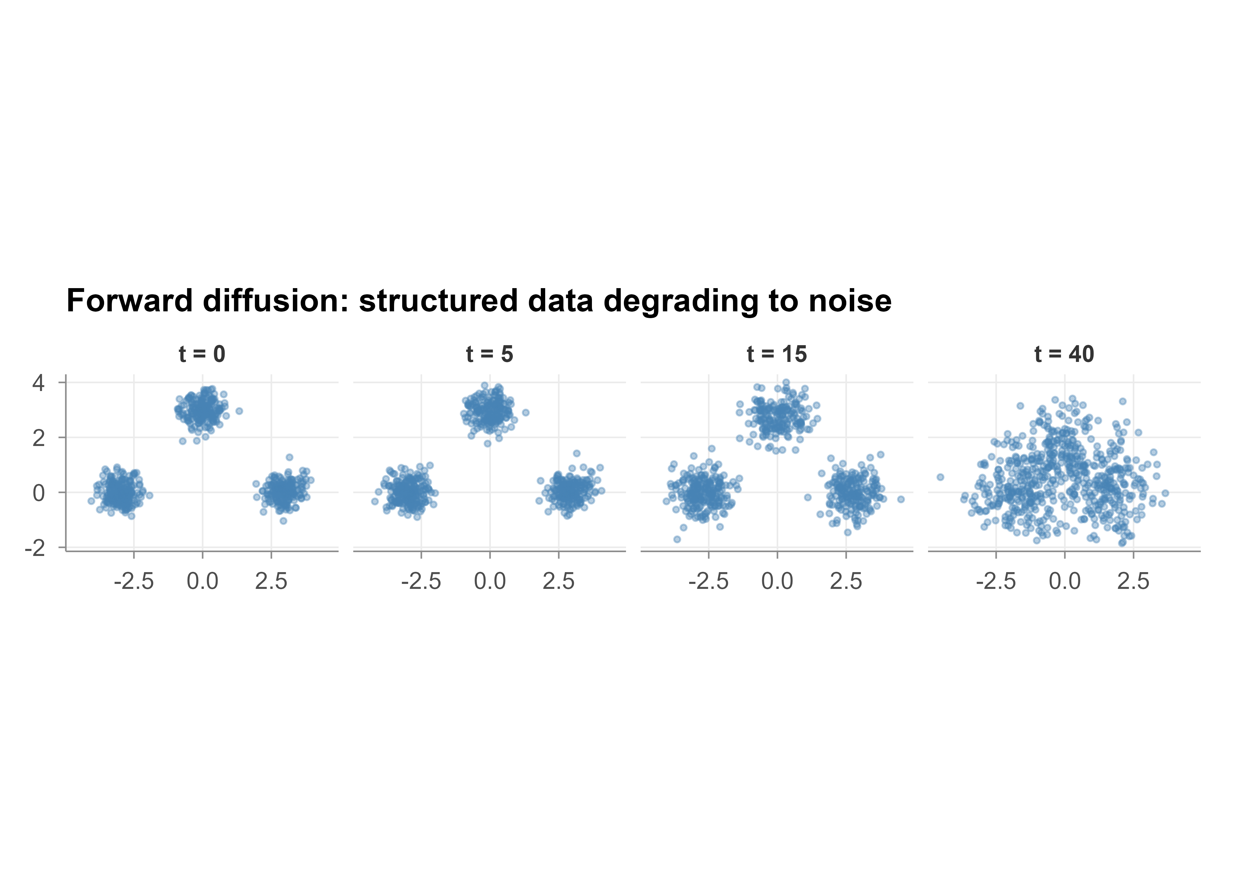
We sample a small mixture of three Gaussians, then apply the closed form \(x_t = \sqrt{\bar\alpha_t}\, x_0 + \sqrt{1 - \bar\alpha_t}\, \epsilon\) at a few timesteps. Figure 42.1 shows the result: the three clear modes at \(t = 0\) dissolve toward a single noise cloud as \(t\) increases.
Show code
# Sample a 2-D Gaussian mixture as the data distribution p(x0)n<-600centers<-matrix(c(-3, 0, 3, 0, 0, 3), ncol =2, byrow =TRUE)comp<-sample(1:3, n, replace =TRUE)x0<-centers[comp, ]+matrix(rnorm(2*n, sd =0.35), ncol =2)# Linear variance schedule and cumulative product alpha_barT_steps<-40beta<-seq(1e-4, 0.06, length.out =T_steps)alpha<-1-betaalpha_bar<-cumprod(alpha)# Apply the closed form at selected stepssteps_to_show<-c(0, 5, 15, 40)make_frame<-function(t){if(t==0){xt<-x0}else{ab<-alpha_bar[t]eps<-matrix(rnorm(2*n), ncol =2)xt<-sqrt(ab)*x0+sqrt(1-ab)*eps}data.frame(x =xt[, 1], y =xt[, 2], step =paste0("t = ", t))}frames<-do.call(rbind, lapply(steps_to_show, make_frame))frames$step<-factor(frames$step, levels =paste0("t = ", steps_to_show))ggplot(frames, aes(x, y))+geom_point(alpha =0.4, size =0.8, color ="steelblue")+facet_wrap(~step, nrow =1)+coord_equal()+labs( title ="Forward diffusion: structured data degrading to noise", x =NULL, y =NULL)
Figure 42.1: Forward diffusion applied to a two dimensional Gaussian mixture. The three modes visible at step zero degrade into standard Gaussian noise by step forty as the closed form mixes in progressively more noise.
At \(t = 0\) the three modes are clear. By \(t = 40\) the cumulative product \(\bar\alpha_t\) is near zero, so the signal is gone and the points look like standard Gaussian noise.
To quantify the loss of structure, we report two summaries per step: the total variance of the cloud, and a Kullback Leibler divergence between the marginal of the first coordinate at step \(t\) and a standard normal, estimated from histograms. Both should move toward the noise reference as \(t\) grows. Table Table 42.1 reports these summaries at selected steps.
Show code
# KL(p || q) for two discrete histograms on a common gridkl_hist<-function(samp, ref_density, breaks){p<-hist(samp, breaks =breaks, plot =FALSE)$densitymids<-head(breaks, -1)+diff(breaks)/2q<-ref_density(mids)p<-p/sum(p)q<-q/sum(q)keep<-p>0&q>0sum(p[keep]*log(p[keep]/q[keep]))}grid<-seq(-6, 6, length.out =41)ref<-function(m)dnorm(m)summ<-lapply(0:T_steps, function(t){if(t==0){xt<-x0}else{ab<-alpha_bar[t]eps<-matrix(rnorm(2*n), ncol =2)xt<-sqrt(ab)*x0+sqrt(1-ab)*eps}data.frame( step =t, total_var =round(sum(apply(xt, 2, var)), 3), kl_to_normal =round(kl_hist(xt[, 1], ref, grid), 3))})diffusion_tab<-do.call(rbind, summ)diffusion_tab<-diffusion_tab[diffusion_tab$step%in%c(0, 5, 10, 20, 30, 40), ]knitr::kable(diffusion_tab, row.names =FALSE, col.names =c("Step t", "Total variance", "KL of x1 to N(0,1)"), caption ="Structure decays as the forward process adds noise.")
Table 42.1: Structure decays as the forward process adds noise.
Step t
Total variance
KL of x1 to N(0,1)
0
8.290
2.509
5
8.172
2.423
10
7.810
2.166
20
6.642
1.402
30
5.283
0.810
40
3.857
0.358
The KL divergence to a standard normal falls steeply over the first several steps and approaches zero, confirming that the marginal becomes standard Gaussian as the chain runs.
42.5.2 Verifying the forward posterior mean
The derivation of the simple loss hinged on the forward posterior \(q(x_{t-1} \mid x_t, x_0)\) being Gaussian with mean \(\tilde\mu_t(x_t, x_0)\). We can confirm that mean numerically without any network. Fix \(x_0\) and a step \(t\), generate many pairs \((x_{t-1}, x_t)\) from the forward chain, then estimate \(\mathbb{E}[x_{t-1} \mid x_t \approx x_t^\star, x_0]\) by averaging the \(x_{t-1}\) whose \(x_t\) landed near a target value, and compare against the closed form.
Show code
t<-20x0_scalar<-2.0at<-alpha[t]abar_t<-alpha_bar[t]abar_tm1<-alpha_bar[t-1]bt<-beta[t]# Closed-form forward posterior mean tilde_mu_t at a chosen x_t = xt_starxt_star<-1.0mu_closed<-(sqrt(abar_tm1)*bt)/(1-abar_t)*x0_scalar+(sqrt(at)*(1-abar_tm1))/(1-abar_t)*xt_star# Monte Carlo: simulate the two-step forward chain from x0, bin on x_tN<-4e6xtm1<-sqrt(abar_tm1)*x0_scalar+sqrt(1-abar_tm1)*rnorm(N)xt<-sqrt(at)*xtm1+sqrt(bt)*rnorm(N)near<-abs(xt-xt_star)<0.02mu_mc<-mean(xtm1[near])knitr::kable(data.frame( quantity =c("closed-form tilde_mu_t", "Monte Carlo estimate"), value =round(c(mu_closed, mu_mc), 4)), col.names =c("Quantity", "Value"), caption ="Closed-form forward posterior mean matches the simulated conditional mean.")
Closed-form forward posterior mean matches the simulated conditional mean.
Quantity
Value
closed-form tilde_mu_t
1.0988
Monte Carlo estimate
1.0975
The two values agree to within Monte Carlo error, confirming the Gaussian posterior mean that the variational bound relies on.
42.5.3 Optimal GAN discriminator as a density ratio
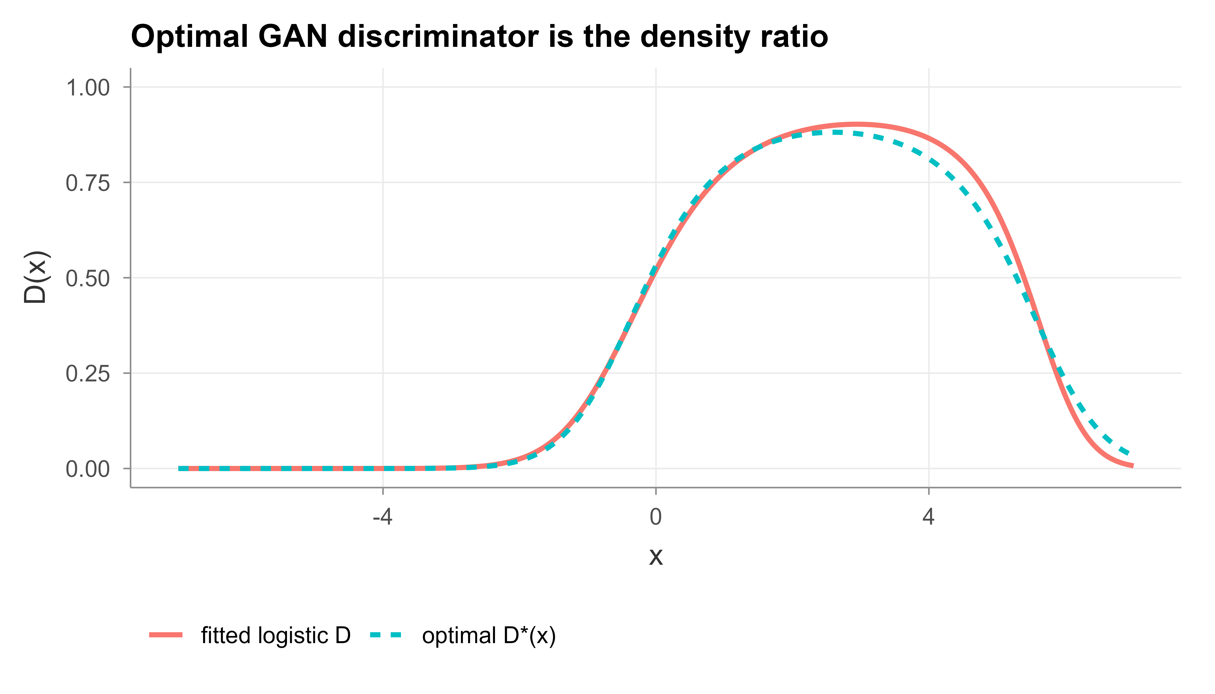
Take real data as \(\mathcal{N}(1, 1)\) and the generator distribution as \(\mathcal{N}(-1, 1.5^2)\). The theory says the best discriminator is \(D^*(x) = p_{\mathrm{data}}(x) / (p_{\mathrm{data}}(x) + p_g(x))\). We compute that curve directly and also fit a discriminator by logistic regression on real versus fake samples to check that the trained classifier recovers the same shape. Figure 42.2 overlays the closed form curve and the fitted classifier.
Show code
# True densitiesp_data<-function(x)dnorm(x, mean =1, sd =1.0)p_g<-function(x)dnorm(x, mean =-1, sd =1.5)xs<-seq(-7, 7, length.out =400)d_star<-p_data(xs)/(p_data(xs)+p_g(xs))# Empirical check: label real = 1, fake = 0, fit logistic regressionm<-4000real<-rnorm(m, mean =1, sd =1.0)fake<-rnorm(m, mean =-1, sd =1.5)df<-data.frame( x =c(real, fake), label =c(rep(1, m), rep(0, m)))fit<-glm(label~poly(x, 4), data =df, family =binomial())d_fit<-predict(fit, newdata =data.frame(x =xs), type ="response")plot_df<-rbind(data.frame(x =xs, D =d_star, source ="optimal D*(x)"),data.frame(x =xs, D =d_fit, source ="fitted logistic D"))ggplot(plot_df, aes(x, D, color =source, linetype =source))+geom_line(linewidth =1)+ylim(0, 1)+labs( title ="Optimal GAN discriminator is the density ratio", x ="x", y ="D(x)", color =NULL, linetype =NULL)+theme(legend.position ="bottom")
Figure 42.2: The optimal GAN discriminator as a density ratio. The closed form curve \(D^*(x) = p_{data}/(p_{data}+p_g)\) and a logistic regression fitted on real versus fake samples coincide, sitting near one where the data density dominates and near zero where the generator density dominates.
The closed form \(D^*\) and the fitted classifier overlap closely. Where the data density dominates, \(D^*\) is near one. Where the generator density dominates, \(D^*\) is near zero. At the crossover point the two densities are equal and \(D^* = 0.5\), which is the point a perfectly trained generator drives the whole curve toward. Table 42.2 confirms numerically that the value at the optimal discriminator equals \(-\log 4 + 2\,D_{\mathrm{JS}}\).
Show code
# Numerically relate the value at D* to Jensen-Shannon divergencemix<-function(x)0.5*(p_data(x)+p_g(x))kl_int<-function(p, q){integrate(function(x){pp<-p(x); qq<-q(x)ifelse(pp>0, pp*log(pp/qq), 0)}, -20, 20)$value}jsd<-0.5*kl_int(p_data, mix)+0.5*kl_int(p_g, mix)value_at_opt<--log(4)+2*jsdknitr::kable(data.frame( quantity =c("JS divergence", "value -log4 + 2*JSD", "-log 4"), value =round(c(jsd, value_at_opt, -log(4)), 4)), col.names =c("Quantity", "Value"), caption ="GAN value at the optimal discriminator equals -log4 + 2 times JS divergence.")
Table 42.2: GAN value at the optimal discriminator equals -log4 + 2 times JS divergence.
Quantity
Value
JS divergence
0.2532
value -log4 + 2*JSD
-0.8799
-log 4
-1.3863
When the two distributions differ, the JS divergence is positive and the generator pays a penalty above the floor of \(-\log 4\). The generator minimizes this penalty by matching \(p_{\mathrm{data}}\), at which point the JS divergence is zero and the value reaches \(-\log 4\).
42.6 Comparison
Now that each family has been seen on its own, it helps to line them up against each other. They trade off sample quality, training stability, whether they give a likelihood, and sampling speed, and no single one wins on every axis. Table Table 42.3 lays out the trade-offs side by side.
Show code
cmp<-data.frame( Property =c("Sample quality","Training stability","Likelihood","Sampling speed","Latent space"), VAE =c("moderate, often blurry","stable","lower bound (ELBO)","fast, one decoder pass","smooth and structured"), GAN =c("sharp, high quality","unstable, mode collapse","none, implicit","fast, one generator pass","usable but less regular"), Diffusion =c("very high quality","stable, simple MSE loss","lower bound, tractable","slow, many denoising steps","no compact latent code"))knitr::kable(cmp, caption ="VAE, GAN, and diffusion at a glance.")
Table 42.3: VAE, GAN, and diffusion at a glance.
Property
VAE
GAN
Diffusion
Sample quality
moderate, often blurry
sharp, high quality
very high quality
Training stability
stable
unstable, mode collapse
stable, simple MSE loss
Likelihood
lower bound (ELBO)
none, implicit
lower bound, tractable
Sampling speed
fast, one decoder pass
fast, one generator pass
slow, many denoising steps
Latent space
smooth and structured
usable but less regular
no compact latent code
In short: VAEs give a clean probabilistic latent space and stable training but softer samples; GANs give sharp samples at the cost of fragile training; and diffusion models give the best samples with stable training but pay for it at sampling time because every sample needs many sequential steps.
When to use this
Reach for a VAE when you want a smooth, interpretable latent space or a likelihood-style score (anomaly detection, representation learning). Reach for a GAN when sharp samples matter more than coverage or stability. Reach for a diffusion model when sample quality is the priority and you can afford slower generation. These trade-offs shift as the field moves, so treat the table as a snapshot rather than a verdict.
42.7 Further Reading
Kingma and Welling (2014), Auto-Encoding Variational Bayes. The original VAE paper with the ELBO and the reparameterization trick.
Goodfellow et al. (2014), Generative Adversarial Nets. Introduces the minimax game and proves the optimal discriminator and JS divergence result.
Sohl-Dickstein et al. (2015), Deep Unsupervised Learning using Nonequilibrium Thermodynamics. The first diffusion model for generative modeling.
Ho et al. (2020), Denoising Diffusion Probabilistic Models. The simplified noise prediction objective used in modern diffusion models.
The full neural network versions need a GPU and the Keras/TensorFlow stack, so those code blocks are shown for reference but not executed here. The base R demonstration captures the key mathematical facts, the forward diffusion process and the optimal GAN discriminator, that you can verify on your own machine.↩︎
The Kullback Leibler divergence \(D_{\mathrm{KL}}(q \| p)\) measures how far one distribution \(q\) is from another \(p\). It is zero when \(q = p\) and positive otherwise, which is why a lower bound that differs from the target by a KL term can never overshoot.↩︎
The Jensen Shannon divergence is a smoothed, symmetric cousin of the KL divergence: \(D_{\mathrm{JS}}(p \| q) = \tfrac12
D_{\mathrm{KL}}(p \| m) + \tfrac12 D_{\mathrm{KL}}(q \| m)\) with \(m = \tfrac12(p +
q)\). Unlike KL it is always finite and symmetric in its two arguments.↩︎
Source Code
# Generative Models {#sec-generative-models}```{r}#| include: falsesource("_common.R")```Imagine you have a folder of ten thousand photographs of faces and you want acomputer to produce a brand new face that no one has ever seen, yet lookscompletely real. A classifier cannot do this. A classifier reads a photo andreturns a label such as "smiling" or "not smiling". It never has to understandwhat makes a face a face. To invent a new one, the computer needs a model ofwhat faces look like in general, not just a rule for telling two kinds apart.That distinction, between a model that *labels* data and a model that can*produce* data, is the subject of this chapter.Most of this book studies discriminative models. A discriminative model learns$p(y \mid x)$ directly: given an input $x$, it returns a label or a number. Agenerative model instead learns the data distribution itself, either the joint$p(x, y)$ or the marginal $p(x)$. Once you have a model of $p(x)$, you can domore than classify. You can draw new samples that look like the training data,score how likely a point is, fill in missing parts of an input, and compressdata into a compact code.::: {.callout-tip title="Intuition"}A discriminative model learns where to draw the line betweencategories. A generative model learns the whole landscape the data live on, soit can walk around and produce new points anywhere on that landscape.:::This chapter covers three families that dominate modern generative modeling:variational autoencoders (VAEs), generative adversarial networks (GANs), anddiffusion models. For each one you will see the intuition first, then the maththat makes it precise, then a sketch of the code, and finally what the resultmeans. The three families reach the same goal, a model you can sample from, byvery different routes, and the closing comparison lays out the trade-offs side byside. The runnable demonstration near the end uses base R and ggplot2 only, soevery number in it reproduces without a deep learning backend.^[The full neuralnetwork versions need a GPU and the Keras/TensorFlow stack, so those code blocksare shown for reference but not executed here. The base R demonstration capturesthe key mathematical facts, the forward diffusion process and the optimal GANdiscriminator, that you can verify on your own machine.]## Generative versus DiscriminativeBefore meeting the three model families, it is worth pinning down precisely what"generative" means and why it is a different job from the classification andregression that occupy much of this book. The cleanest way in is to write thejoint distribution two ways:$$p(x, y) = p(y \mid x)\, p(x) = p(x \mid y)\, p(y).$$A discriminative model targets the first factor $p(y \mid x)$ and ignores$p(x)$. Logistic regression, random forests, and the neural network classifiersfrom earlier chapters all sit here. They tend to predict well because they spendall of their capacity on the boundary between classes.A generative model targets $p(x \mid y)$ and $p(y)$, or just $p(x)$ when thereare no labels. Classification then comes from Bayes rule,$$p(y \mid x) = \frac{p(x \mid y)\, p(y)}{\sum_{y'} p(x \mid y')\, p(y')}.$$Naive Bayes (@sec-naive-bayes) and Gaussian discriminant analysis(@sec-discriminant-analysis) are classic examples. Modeling$p(x)$ is harder than modeling a boundary, because the model has to account foreverything in the data, not just the part that separates classes. So why paythat price? Classification is only one of several payoffs. A model of $p(x)$ letsyou:- sample new data, for example images, audio, or molecules,- detect outliers as points with low $p(x)$ (@sec-anomaly-detection),- impute missing features,- learn a useful low dimensional representation,- augment a small training set with synthetic examples.::: {.callout-note}None of the three families below require the labels $y$. They learnthe shape of $p(x)$ from inputs alone, which is why they are usually trained onunlabeled data, of which the world has far more than labeled data.:::The three families take different routes to a model you can sample from. We startwith the one closest to ideas already in this book, the autoencoder.## Variational AutoencodersThe first family stays closest to familiar territory. A variational autoencoder(VAE) is a latent variable model: it assumes each observed point $x$ is generatedfrom an unobserved, low dimensional code $z$ that we never see directly. Thegenerative story is$$z \sim p(z) = \mathcal{N}(0, I), \qquad x \sim p_\theta(x \mid z),$$so the marginal likelihood of a data point integrates over the latent variable,$$p_\theta(x) = \int p_\theta(x \mid z)\, p(z)\, dz .$$Here $z$ is the *latent code*, a short vector that captures the essence of $x$(say, a handful of numbers summarizing a face), and $p_\theta(x \mid z)$ is the*decoder*, the network with parameters $\theta$ that turns a code back into adata point.This connects to the autoencoders chapter (@sec-autoencoders). Aplain autoencoder maps $x$ to a code and back with no probabilistic meaning. AVAE keeps the encoder and decoder shape but makes both stochastic, which lets ussample new $x$ by drawing $z \sim \mathcal{N}(0, I)$ and passing it through thedecoder.::: {.callout-important title="Key idea"}A plain autoencoder compresses and reconstructs. A VAE turns thatsame architecture into a generator by insisting the codes follow a knowndistribution, the standard normal, so you can sample a fresh code and decode itinto a new, plausible $x$.:::### The problem with the integralThere is a snag. To train the model we would like to maximize $p_\theta(x)$, butthe integral over $z$ has no closed form for a neural network decoder, and theposterior $p_\theta(z \mid x) = p_\theta(x \mid z)\, p(z) / p_\theta(x)$ (whichcodes are likely to have produced a given $x$) is equally hard. The VAE worksaround both by introducing a second network, an encoder $q_\phi(z \mid x)$, that*approximates* the true posterior. The encoder outputs a mean and a variance,$$q_\phi(z \mid x) = \mathcal{N}\!\big(\mu_\phi(x),\, \mathrm{diag}(\sigma_\phi^2(x))\big).$$### The evidence lower boundBecause we cannot maximize $\log p_\theta(x)$ directly, we maximize a quantitythat is guaranteed to sit just below it and is computable. Start from the logmarginal likelihood and insert $q_\phi$:$$\log p_\theta(x)= \log \int p_\theta(x \mid z)\, p(z)\, dz= \log \mathbb{E}_{q_\phi(z \mid x)}\!\left[\frac{p_\theta(x \mid z)\, p(z)}{q_\phi(z \mid x)}\right].$$Jensen inequality moves the log inside the expectation and gives a lower bound,the evidence lower bound or ELBO:$$\log p_\theta(x) \ge \mathbb{E}_{q_\phi(z \mid x)}\big[\log p_\theta(x \mid z)\big]- D_{\mathrm{KL}}\!\big(q_\phi(z \mid x)\,\|\,p(z)\big) =: \mathcal{L}(\theta, \phi; x).$$It is worth deriving the same bound a second way, by an exact identity ratherthan an inequality, because the algebra reveals precisely what is lost. For any$q_\phi(z \mid x)$ with the same support as the posterior, multiply and divideinside the log and split the expectation:$$\begin{aligned}\log p_\theta(x)&= \mathbb{E}_{q_\phi(z \mid x)}\big[\log p_\theta(x)\big] \\&= \mathbb{E}_{q_\phi}\!\left[\log \frac{p_\theta(x, z)}{p_\theta(z \mid x)}\right] \\&= \mathbb{E}_{q_\phi}\!\left[\log \frac{p_\theta(x, z)}{q_\phi(z \mid x)}\right] + \mathbb{E}_{q_\phi}\!\left[\log \frac{q_\phi(z \mid x)}{p_\theta(z \mid x)}\right] \\&= \mathcal{L}(\theta, \phi; x) + D_{\mathrm{KL}}\!\big(q_\phi(z \mid x)\,\|\,p_\theta(z \mid x)\big),\end{aligned}$$ {#eq-generative-models-elbo-decomp}where the first line uses that $\log p_\theta(x)$ does not depend on $z$, thesecond uses $p_\theta(x) = p_\theta(x, z) / p_\theta(z \mid x)$, and the last linerecognizes $\mathbb{E}_{q_\phi}[\log p_\theta(x, z) - \log q_\phi] = \mathcal{L}$once $p_\theta(x, z) = p_\theta(x \mid z)\, p(z)$ is expanded. Equation@eq-generative-models-elbo-decomp is exact: the log evidence equals the ELBOplus a non negative KL term, so the ELBO is a lower bound, and the inequality istight exactly when $q_\phi$ equals the true posterior.The gap between $\log p_\theta(x)$ and the ELBO is exactly$D_{\mathrm{KL}}(q_\phi(z \mid x)\,\|\,p_\theta(z \mid x))$, which is nonnegative,^[The Kullback Leibler divergence $D_{\mathrm{KL}}(q \| p)$ measures howfar one distribution $q$ is from another $p$. It is zero when $q = p$ andpositive otherwise, which is why a lower bound that differs from the target by aKL term can never overshoot.] so maximizing $\mathcal{L}$ does two good things atonce: it pushes the bound up and it makes the approximate posterior close to thetrue one.Read the two terms as a loss. The first term is a reconstruction term: itrewards a decoder that assigns high probability to the actual $x$ given its code.The second term is a Kullback Leibler penalty that pulls the encodeddistribution toward the prior $\mathcal{N}(0, I)$. The KL term acts as aregularizer. Without it the encoder could place every input in its own tinyregion of latent space, which would reconstruct well but leave gaps that decodeto nothing. The penalty keeps the latent space packed near the prior so thatrandom draws decode into plausible samples.::: {.callout-tip title="Intuition"}Picture the reconstruction term as "remember the data" and theKL term as "stay tidy". Pull only on the first and the model memorizes inputsinto scattered, unusable codes. Pull only on the second and every inputcollapses to the same blurry average. The ELBO balances the two.:::When both $q_\phi(z \mid x)$ and $p(z)$ are Gaussian the KL term has a closedform, so there is nothing to estimate by sampling. For a $d$ dimensional diagonal Gaussian,$$D_{\mathrm{KL}}\!\big(\mathcal{N}(\mu, \sigma^2 I)\,\|\,\mathcal{N}(0, I)\big)= \tfrac{1}{2} \sum_{j=1}^{d} \big(\mu_j^2 + \sigma_j^2 - \log \sigma_j^2 - 1\big).$$ {#eq-generative-models-gauss-kl}The closed form is worth deriving once, because it explains why each term has thesign it does. The KL divergence between two univariate Gaussians$\mathcal{N}(\mu_1, \sigma_1^2)$ and $\mathcal{N}(\mu_2, \sigma_2^2)$ is$$D_{\mathrm{KL}}= \mathbb{E}_{q}\!\left[\log \frac{q(z)}{p(z)}\right]= \mathbb{E}_q\!\left[\log\frac{\sigma_2}{\sigma_1} - \frac{(z - \mu_1)^2}{2\sigma_1^2} + \frac{(z - \mu_2)^2}{2\sigma_2^2}\right].$$Under $q$ we have $\mathbb{E}_q[(z - \mu_1)^2] = \sigma_1^2$ and$\mathbb{E}_q[(z - \mu_2)^2] = \sigma_1^2 + (\mu_1 - \mu_2)^2$, so the expectationcollapses to$$D_{\mathrm{KL}} = \log\frac{\sigma_2}{\sigma_1} + \frac{\sigma_1^2 + (\mu_1 - \mu_2)^2}{2\sigma_2^2} - \frac12 .$$Setting the prior to the standard normal, $\mu_2 = 0$ and $\sigma_2 = 1$, andsumming over the $d$ independent coordinates of the diagonal posterior gives@eq-generative-models-gauss-kl. The quadratic terms $\mu_j^2$ and $\sigma_j^2$penalize codes that drift from the origin or spread too wide, while the$-\log \sigma_j^2$ term forbids the variance from collapsing to zero, which wouldmake the posterior a point mass and the latent space unusable for sampling.::: {.callout-warning title="Posterior collapse"}A characteristic VAE failure is posterior collapse, where for some latentcoordinates the encoder ignores the input and returns$q_\phi(z_j \mid x) \approx p(z_j) = \mathcal{N}(0, 1)$, driving the KL term in@eq-generative-models-gauss-kl to zero. The decoder then learns to reconstructwithout using those coordinates, so they carry no information. This happens mostoften when the decoder is powerful enough to model $x$ on its own (for example anautoregressive decoder) and early in training when the reconstruction term isweak. Standard remedies are KL annealing (warm up the KL weight from zero), freebits (clamp each coordinate's KL at a small floor $\lambda$ so the optimizer stopsshrinking it once it is informative enough), or the $\beta$-VAE weighting below.:::### Amortized inference and the $\beta$-VAEThe encoder $q_\phi(z \mid x)$ deserves a second look. Classical variationalinference fits a separate set of variational parameters $(\mu_i, \sigma_i)$ forevery data point $x_i$, solving an optimization per example. The VAE insteadtrains a single network that maps any $x$ to its $(\mu_\phi(x), \sigma_\phi(x))$,sharing parameters across the whole dataset. This is amortized inference: the costof inference is amortized over the dataset by paying once to train the encoder,after which a new point's approximate posterior is a single forward pass. Theprice is the amortization gap, the extra slack between the ELBO achieved by theshared encoder and the best ELBO a per example optimizer could reach. Togetherwith the approximation gap from $q_\phi$ being Gaussian rather than the trueposterior, this is why the ELBO can sit well below $\log p_\theta(x)$.The full training objective is the ELBO averaged over the data, and the gradientwith respect to $\theta$ and $\phi$ is estimated by drawing a minibatch and onereparameterized $\epsilon$ per example. A widely used generalization scales the KLterm by a constant $\beta$,$$\mathcal{L}_\beta(\theta, \phi; x)= \mathbb{E}_{q_\phi(z \mid x)}\big[\log p_\theta(x \mid z)\big]- \beta\, D_{\mathrm{KL}}\!\big(q_\phi(z \mid x)\,\|\,p(z)\big).$$ {#eq-generative-models-beta-vae}With $\beta = 1$ this is the exact ELBO. Setting $\beta > 1$ presses theaggregated posterior harder toward the factorized prior, which tends to producemore disentangled latent coordinates at the cost of reconstruction fidelity, while$\beta < 1$ favors sharper reconstructions and risks the scattered, gap riddledlatent space the KL term is meant to prevent. The reconstruction term has its ownimplicit weight: with a Gaussian decoder of fixed variance $\sigma_x^2$, thenegative log likelihood is $\|x - \hat x\|^2 / (2\sigma_x^2)$ up to a constant, so$\sigma_x^2$ acts as an inverse weight on reconstruction relative to the KL term.This is why a plain mean squared error decoder with no explicit varianceimplicitly fixes a particular trade-off.### The reparameterization trickTo train with gradient descent we need gradients of $\mathcal{L}$ with respectto the encoder parameters $\phi$. The trouble is that the expectation is takenover a distribution that depends on $\phi$, so we cannot just sample $z$ andbackpropagate through the sampling step. The reparameterization trick rewritesthe sample as a deterministic function of $\phi$ plus external noise,$$z = \mu_\phi(x) + \sigma_\phi(x) \odot \epsilon, \qquad \epsilon \sim \mathcal{N}(0, I),$$where $\odot$ is elementwise multiplication. Now the randomness lives in$\epsilon$, which does not depend on $\phi$, and the path from $\phi$ to $z$ isdifferentiable. The Monte Carlo estimate of the ELBO using one or a few draws of$\epsilon$ then has a well defined gradient.To see precisely why this matters, compare two ways of differentiating anexpectation $\mathbb{E}_{q_\phi(z)}[f(z)]$ whose distribution depends on $\phi$.The score function or REINFORCE estimator uses the identity$\nabla_\phi q_\phi = q_\phi\, \nabla_\phi \log q_\phi$ to write$$\nabla_\phi \mathbb{E}_{q_\phi}[f(z)]= \mathbb{E}_{q_\phi}\!\big[f(z)\, \nabla_\phi \log q_\phi(z)\big],$$which is unbiased and needs only $\log q_\phi$, not a differentiable $f$, but isnotoriously high variance because $f(z)$ multiplies the score with nocancellation. The reparameterization estimator instead pushes the parameterinside a deterministic map $z = g_\phi(\epsilon)$ with $\epsilon \sim p(\epsilon)$fixed, giving$$\nabla_\phi \mathbb{E}_{q_\phi}[f(z)]= \mathbb{E}_{p(\epsilon)}\!\big[\nabla_\phi f(g_\phi(\epsilon))\big]= \mathbb{E}_{p(\epsilon)}\!\big[f'(z)\, \nabla_\phi g_\phi(\epsilon)\big].$$The Jacobian $\nabla_\phi g_\phi$ couples the gradient of $f$ directly to theparameter, so the estimator exploits the smoothness of the decoder and typicallyhas far lower variance, often by orders of magnitude. The cost is that it requires$f$ (here the integrand of the ELBO) to be differentiable in $z$, which holds forcontinuous data and a Gaussian $q_\phi$ but fails for discrete $z$, where onefalls back on the score function estimator or a continuous relaxation such as theGumbel-Softmax.::: {.callout-important title="Key idea"}You cannot differentiate through "draw a random sample", but youcan differentiate through "scale and shift a fixed random sample". Thereparameterization trick is exactly that move, and it is what makes the VAEtrainable by ordinary backpropagation.:::The next block sketches a VAE in Keras. It is shown for reference and is marked`eval = FALSE` because it needs the Keras/TensorFlow backend, which is notavailable in this build.```{r vae-keras, eval = FALSE}library(keras)latent_dim <-2# Encoder outputs mean and log variance of q(z | x)encoder_in <-layer_input(shape =784)h <- encoder_in %>%layer_dense(256, activation ="relu")z_mean <- h %>%layer_dense(latent_dim)z_log_var <- h %>%layer_dense(latent_dim)# Reparameterization: z = mean + exp(log_var / 2) * epsilonsampling <-function(args) { z_mean <- args[[1]] z_log_var <- args[[2]] eps <-k_random_normal(shape =k_shape(z_mean)) z_mean +k_exp(0.5* z_log_var) * eps}z <-list(z_mean, z_log_var) %>%layer_lambda(sampling)# Decoder maps z back to xdecoder <-keras_model_sequential() %>%layer_dense(256, activation ="relu", input_shape = latent_dim) %>%layer_dense(784, activation ="sigmoid")x_decoded <-decoder(z)vae <-keras_model(encoder_in, x_decoded)# Loss = reconstruction + KL regularizerrecon <-784*loss_binary_crossentropy(encoder_in, x_decoded)kl <--0.5*k_sum(1+ z_log_var -k_square(z_mean) -k_exp(z_log_var), axis =-1L)vae$add_loss(k_mean(recon + kl))vae %>%compile(optimizer ="adam")```## Generative Adversarial NetworksThe VAE works hard to keep an explicit, if approximate, handle on thelikelihood. A generative adversarial network (GAN) throws that away and asks adifferent question: instead of "how probable is this data point?", it asks "cananyone tell my fakes from the real thing?" Think of an art forger and adetective. The forger (the generator) paints fakes; the detective (thediscriminator) tries to spot them. Each makes the other better. When the forgerfinally wins, the fakes are indistinguishable from genuine work.Concretely, two networks compete. A generator $G$ maps noise $z \sim p(z)$ to afake sample $G(z)$. A discriminator $D$ takes a sample and outputs theprobability that it is real. Training is a minimax game,$$\min_G \max_D \;\mathbb{E}_{x \sim p_{\mathrm{data}}}\big[\log D(x)\big]+ \mathbb{E}_{z \sim p_z}\big[\log\big(1 - D(G(z))\big)\big].$$The discriminator wants to push $D(x)$ toward one on real data and toward zeroon fakes. The generator wants the opposite, to make $D(G(z))$ close to one. The$\min_G \max_D$ notation reads literally: the inner $\max_D$ trains the bestdetective it can, and the outer $\min_G$ trains the forger to defeat that bestdetective.::: {.callout-note}A GAN never writes down or evaluates $p(x)$. It is an *implicit*generative model: it can hand you samples but cannot tell you how likely anyparticular point is. That is the price of skipping the likelihood.:::### The optimal discriminatorIt helps to ask what the perfect detective would do, holding the forger fixed.Fix the generator, so the distribution of fakes $p_g$ is fixed. Write the valuefunction as a single integral over $x$,$$V(D) = \int_x \Big( p_{\mathrm{data}}(x) \log D(x) + p_g(x) \log\big(1 - D(x)\big) \Big)\, dx .$$For each $x$ the integrand has the form $a \log d + b \log(1 - d)$, which ismaximized at $d = a / (a + b)$. The optimal discriminator is therefore thedensity ratio$$D^*(x) = \frac{p_{\mathrm{data}}(x)}{p_{\mathrm{data}}(x) + p_g(x)} .$$Substitute $D^*$ back into the value function. After collecting terms it becomes$$V(G, D^*) = -\log 4 + 2\, D_{\mathrm{JS}}\!\big(p_{\mathrm{data}} \,\|\, p_g\big),$$ {#eq-generative-models-gan-js}The collecting of terms is short enough to show. Write $m = \tfrac12(p_{\mathrm{data}} + p_g)$ for the mixture. Substituting $D^* = p_{\mathrm{data}} / (2m)$ and$1 - D^* = p_g / (2m)$ gives$$\begin{aligned}V(G, D^*)&= \mathbb{E}_{p_{\mathrm{data}}}\!\left[\log \frac{p_{\mathrm{data}}}{2m}\right] + \mathbb{E}_{p_g}\!\left[\log \frac{p_g}{2m}\right]\\&= \mathbb{E}_{p_{\mathrm{data}}}\!\left[\log \frac{p_{\mathrm{data}}}{m}\right] + \mathbb{E}_{p_g}\!\left[\log \frac{p_g}{m}\right] - 2\log 2 \\&= D_{\mathrm{KL}}(p_{\mathrm{data}} \,\|\, m) + D_{\mathrm{KL}}(p_g \,\|\, m) - 2\log 2 \\&= 2\, D_{\mathrm{JS}}(p_{\mathrm{data}} \,\|\, p_g) - \log 4,\end{aligned}$$using $D_{\mathrm{JS}}(p \| q) = \tfrac12 D_{\mathrm{KL}}(p \| m) + \tfrac12 D_{\mathrm{KL}}(q \| m)$ in the last line. This is@eq-generative-models-gan-js. Because $D_{\mathrm{JS}} \ge 0$ with equalityiff $p_g = p_{\mathrm{data}}$, the outer minimization over $G$ drives $p_g$ to thedata distribution and the value to its floor $-\log 4$.where $D_{\mathrm{JS}}$ is the Jensen Shannon divergence, a symmetric measure ofhow far two distributions are apart.^[The Jensen Shannon divergence is a smoothed,symmetric cousin of the KL divergence: $D_{\mathrm{JS}}(p \| q) = \tfrac12D_{\mathrm{KL}}(p \| m) + \tfrac12 D_{\mathrm{KL}}(q \| m)$ with $m = \tfrac12(p +q)$. Unlike KL it is always finite and symmetric in its two arguments.] Since theJS divergence is zero only when $p_g = p_{\mathrm{data}}$, the generator thatwins the game matches the data distribution exactly, with the value reaching itsminimum of $-\log 4$.::: {.callout-important title="Key idea"}Underneath the forger-versus-detective story, the GAN issecretly minimizing a divergence between the fake and real distributions. Theadversarial game is just a clever, sample-only way to estimate and descend thatdivergence without ever computing a density.:::The demonstration below evaluates $D^*(x)$ for two Gaussians so the density ratioresult is visible as a concrete curve.### Mode collapse and instabilityThe clean theory above assumes both networks are trained to optimality at eachstep, which never happens in practice. Two failures are common, and knowing theirnames is half of diagnosing a misbehaving GAN.The first is *mode collapse*: the generator discovers a few outputs that reliablyfool the current discriminator and produces only those, ignoring whole regions ofthe data. The samples look fine one at a time but lack variety, like a forger whoonly knows how to paint one convincing painting.The second is *training instability*: the two networks chase a moving target. Ifthe discriminator gets too strong, the term $\log(1 - D(G(z)))$ saturates and thegenerator gradient vanishes, so the forger stops learning precisely when it islosing badly. A common fix is to have the generator maximize $\log D(G(z))$instead, which gives stronger gradients early in training. Balancing the twonetworks, tuning learning rates, and choosing alternative losses such as theWasserstein objective are all standard parts of getting a GAN to converge.The saturation is easy to make precise. Let $u = D(G(z))$ be the discriminator'sprobability that a fake is real, small early in training when fakes are obvious.The original generator loss $\log(1 - u)$ has derivative $-1/(1 - u)$, which isnear $-1$ when $u \approx 0$: a tiny, nearly constant gradient exactly when thegenerator most needs a push. The non saturating surrogate maximizes $\log u$,whose derivative $1/u$ blows up as $u \to 0$, supplying a large gradient when thefakes are poor. Both losses share the same fixed point but have opposite gradientbehavior in the regime that matters early on, which is why the non saturating formis the practical default.### Why JS divergence is a brittle objectiveThe JS divergence result @eq-generative-models-gan-js is elegant but alsodiagnoses the deeper instability. When $p_{\mathrm{data}}$ and $p_g$ live onlow dimensional manifolds in a high dimensional space, as natural images do, theirsupports are almost surely disjoint or overlap on a set of measure zero early intraining. On disjoint supports a perfect discriminator exists, $D_{\mathrm{JS}}$is pinned at its maximum $\log 2$ regardless of how far apart the twodistributions are, and its gradient with respect to the generator is zero almosteverywhere. The generator receives no signal about which direction would move$p_g$ toward $p_{\mathrm{data}}$. This is the manifold view of why a too strongdiscriminator kills learning.The Wasserstein GAN replaces JS with the earth mover (Wasserstein-1) distance,which by Kantorovich-Rubinstein duality equals$$W(p_{\mathrm{data}}, p_g)= \sup_{\|f\|_L \le 1} \;\mathbb{E}_{p_{\mathrm{data}}}[f(x)] - \mathbb{E}_{p_g}[f(x)],$$ {#eq-generative-models-wgan}where the supremum is over all 1-Lipschitz functions $f$. Unlike JS, $W$ variessmoothly with the distance between $p_g$ and $p_{\mathrm{data}}$ even when theirsupports do not overlap, so it provides a usable gradient everywhere. In practice$f$ (now called a critic, with no sigmoid and a real valued output) is constrainedto be Lipschitz by weight clipping or, more reliably, a gradient penalty thatpushes $\|\nabla_x f\|$ toward one. The critic loss in@eq-generative-models-wgan also tracks sample quality, which the original GANloss does not, so it partially answers the warning below.::: {.callout-warning}Unlike the VAE loss, a GAN loss curve does not tell you much. Thegenerator and discriminator losses can stay flat while sample quality improvesor collapses. Judge a GAN by looking at its samples, not by watching the lossgo down.:::A minimal GAN training loop in Keras follows. It is marked `eval = FALSE` becauseit needs the Keras/TensorFlow backend.```{r gan-keras, eval = FALSE}library(keras)generator <-keras_model_sequential() %>%layer_dense(128, activation ="relu", input_shape =100) %>%layer_dense(784, activation ="tanh")discriminator <-keras_model_sequential() %>%layer_dense(128, activation ="relu", input_shape =784) %>%layer_dense(1, activation ="sigmoid")discriminator %>%compile(optimizer ="adam", loss ="binary_crossentropy")# Combined model trains the generator with the discriminator frozenfreeze_weights(discriminator)gan_in <-layer_input(shape =100)gan_out <- gan_in %>%generator() %>%discriminator()gan <-keras_model(gan_in, gan_out)gan %>%compile(optimizer ="adam", loss ="binary_crossentropy")# Each step: update D on real plus fake, then update G through the frozen D.```## Diffusion ModelsHere is a different idea entirely. Take a clear photo and add a tiny bit ofstatic noise, then a little more, then more, until after many steps nothing isleft but television snow. That destruction is easy and needs no learning. Nowsuppose you could run the tape backward, removing a little noise at each step. Ifyou could learn that one denoising step, you could start from pure static andwalk all the way back to a brand new clear photo. That is the whole idea of adiffusion model.Diffusion models generate data by learning to reverse a gradual noising process.The idea goes back to Sohl-Dickstein et al. (2015) and was turned into apractical image generator by Ho et al. (2020). The forward process slowlydestroys structure in the data by adding Gaussian noise over $T$ steps. Thereverse process, learned by a network, removes noise one step at a time, turningpure noise back into a sample.::: {.callout-tip title="Intuition"}Noising is trivial and requires no model. The model only has tolearn the *reverse*, and because each reverse step undoes just a sliver ofnoise, it is a much easier task than producing a whole image in one shot.:::### Forward noising processFix a variance schedule $\beta_1, \dots, \beta_T$ with small positive values.The forward process is a Markov chain that adds a little noise at each step,$$q(x_t \mid x_{t-1}) = \mathcal{N}\!\big(\sqrt{1 - \beta_t}\, x_{t-1},\; \beta_t I\big).$$The scaling by $\sqrt{1 - \beta_t}$ shrinks the previous value just enough thatthe variance stays controlled as noise accumulates, rather than growing withoutbound. After many steps $x_T$ is essentially standard Gaussian noise with allstructure gone.### Closed form for any stepSimulating the chain step by step would be slow during training. A convenientproperty rescues us: you can jump from the clean data $x_0$ to any noised version$x_t$ in a single shot, without running the intermediate steps. Let$\alpha_t = 1 - \beta_t$ and$\bar{\alpha}_t = \prod_{s=1}^{t} \alpha_s$. Then$$q(x_t \mid x_0) = \mathcal{N}\!\big(\sqrt{\bar{\alpha}_t}\, x_0,\; (1 - \bar{\alpha}_t) I\big),$$which can be written with an explicit noise variable,$$x_t = \sqrt{\bar{\alpha}_t}\, x_0 + \sqrt{1 - \bar{\alpha}_t}\, \epsilon, \qquad \epsilon \sim \mathcal{N}(0, I).$$As $t$ grows, $\bar{\alpha}_t \to 0$, so the signal $\sqrt{\bar{\alpha}_t}\, x_0$fades and the noise term takes over.The closed form follows from composing two Gaussian steps. Write$x_t = \sqrt{\alpha_t}\, x_{t-1} + \sqrt{1 - \alpha_t}\, \epsilon_{t-1}$ withindependent $\epsilon_{t-1} \sim \mathcal{N}(0, I)$. Substitute the same identityfor $x_{t-1}$:$$x_t = \sqrt{\alpha_t \alpha_{t-1}}\, x_{t-2} + \sqrt{\alpha_t (1 - \alpha_{t-1})}\, \epsilon_{t-2} + \sqrt{1 - \alpha_t}\, \epsilon_{t-1}.$$The last two terms are independent zero mean Gaussians, so they sum to a singleGaussian whose variance is the sum of variances,$\alpha_t(1 - \alpha_{t-1}) + (1 - \alpha_t) = 1 - \alpha_t \alpha_{t-1}$. Hence$x_t = \sqrt{\alpha_t \alpha_{t-1}}\, x_{t-2} + \sqrt{1 - \alpha_t \alpha_{t-1}}\, \bar\epsilon$with $\bar\epsilon \sim \mathcal{N}(0, I)$. Iterating this merging of Gaussians allthe way down to $x_0$ replaces the product of step coefficients with$\bar\alpha_t = \prod_{s=1}^t \alpha_s$ and leaves total variance$1 - \bar\alpha_t$, which is exactly the stated closed form. The choice of scalingby $\sqrt{1 - \beta_t}$ rather than any other constant is what makes the noisedvariance telescope to $1 - \bar\alpha_t$ and keeps $\mathrm{Var}(x_t)$ bounded byone when the data are standardized.::: {.callout-tip}This closed form is also what makes the runnable demonstration cheap.To show data dissolving at step $t$, we never simulate $t$ separate noisingsteps. We apply the one formula above once.:::The simulation later in the chapter uses exactly this closed form to push twodimensional data toward noise.### Reverse denoising modelTo generate, we run the chain backward. The reverse step is also modeled as aGaussian,$$p_\theta(x_{t-1} \mid x_t) = \mathcal{N}\!\big(\mu_\theta(x_t, t),\; \Sigma_\theta(x_t, t)\big),$$with the mean produced by a network. Training the reverse process can be derivedas a variational bound similar to the ELBO, but Ho et al. (2020) showed asimpler reparameterization. Rather than predicting the mean directly, the networkpredicts the noise $\epsilon$ that was added. Given the closed form above, anetwork $\epsilon_\theta(x_t, t)$ is trained to recover that noise, and thetraining objective collapses to a plain regression on the noise,$$\mathcal{L}_{\mathrm{simple}}(\theta) = \mathbb{E}_{x_0, \epsilon, t}\Big[\big\| \epsilon - \epsilon_\theta\big(\sqrt{\bar{\alpha}_t}\, x_0 + \sqrt{1 - \bar{\alpha}_t}\, \epsilon,\; t\big)\big\|^2\Big].$$ {#eq-generative-models-simple-loss}### From the variational bound to the simple lossThe simple objective is not an ad hoc choice, it is a reweighted version of agenuine ELBO. The variational bound on the negative log likelihood factors overthe chain into three groups of terms,$$-\log p_\theta(x_0) \le \mathbb{E}_q\Big[\underbrace{D_{\mathrm{KL}}(q(x_T \mid x_0) \,\|\, p(x_T))}_{L_T}+ \sum_{t > 1} \underbrace{D_{\mathrm{KL}}(q(x_{t-1} \mid x_t, x_0) \,\|\, p_\theta(x_{t-1} \mid x_t))}_{L_{t-1}}\underbrace{- \log p_\theta(x_0 \mid x_1)}_{L_0}\Big],$$ {#eq-generative-models-diff-elbo}obtained by the same multiply-and-divide trick used for the VAE, now applied tothe joint over the whole trajectory $x_{1:T}$. The term $L_T$ has no learnableparameters (the forward process is fixed and $x_T$ is essentially the prior$\mathcal{N}(0, I)$), so it is a constant. Each $L_{t-1}$ compares the learnedreverse step against the forward posterior $q(x_{t-1} \mid x_t, x_0)$, which,crucially, is Gaussian in closed form. By Bayes rule applied to the Gaussianforward steps,$$q(x_{t-1} \mid x_t, x_0) = \mathcal{N}\!\big(\tilde\mu_t(x_t, x_0),\; \tilde\beta_t I\big),\qquad\tilde\beta_t = \frac{1 - \bar\alpha_{t-1}}{1 - \bar\alpha_t}\,\beta_t,$$with posterior mean$$\tilde\mu_t(x_t, x_0)= \frac{\sqrt{\bar\alpha_{t-1}}\,\beta_t}{1 - \bar\alpha_t}\, x_0 + \frac{\sqrt{\alpha_t}\,(1 - \bar\alpha_{t-1})}{1 - \bar\alpha_t}\, x_t .$$Because both distributions in $L_{t-1}$ are Gaussian with the same (fixed)covariance, the KL reduces to a scaled squared distance between their means,$L_{t-1} = \tfrac{1}{2\tilde\beta_t}\|\tilde\mu_t - \mu_\theta(x_t, t)\|^2 + \text{const}$.Now substitute the closed form $x_0 = (x_t - \sqrt{1 - \bar\alpha_t}\,\epsilon)/\sqrt{\bar\alpha_t}$into $\tilde\mu_t$ and parameterize the network's mean in the matching form$$\mu_\theta(x_t, t)= \frac{1}{\sqrt{\alpha_t}}\Big(x_t - \frac{\beta_t}{\sqrt{1 - \bar\alpha_t}}\, \epsilon_\theta(x_t, t)\Big).$$ {#eq-generative-models-mu-eps}The two means then differ only through $\epsilon - \epsilon_\theta$, and thesquared difference becomes$$L_{t-1} = \frac{\beta_t^2}{2\tilde\beta_t\,\alpha_t (1 - \bar\alpha_t)}\big\|\epsilon - \epsilon_\theta(x_t, t)\big\|^2 + \text{const}.$$ {#eq-generative-models-Lt-weighted}This is the per timestep noise prediction loss, weighted by a $t$ dependentfactor. Ho et al. (2020) found that simply dropping that factor (setting it toone) and averaging over $t$ uniformly, which yields exactly@eq-generative-models-simple-loss, trains better and is the form used inpractice. The reweighting downweights the very small $t$ terms, which correspondto imperceptible high frequency detail, and lets the network spend capacity on theharder, more visually important denoising at larger $t$.In words, the network is shown a noised point and the timestep it came from, andits only job is to guess the noise that was mixed in. Sampling then alternates adenoising step using $\epsilon_\theta$ with a small injection of fresh noise,from $t = T$ down to $t = 1$.The sampling step is the reverse parameterization @eq-generative-models-mu-epsmade concrete. Starting from $x_T \sim \mathcal{N}(0, I)$, each step computes$$x_{t-1} = \frac{1}{\sqrt{\alpha_t}}\Big(x_t - \frac{\beta_t}{\sqrt{1 - \bar\alpha_t}}\, \epsilon_\theta(x_t, t)\Big) + \sigma_t\, z, \qquad z \sim \mathcal{N}(0, I),$$ {#eq-generative-models-sampler}with $z = 0$ on the final step. The injected variance is typically$\sigma_t^2 = \tilde\beta_t$ or the simpler $\sigma_t^2 = \beta_t$; both areconsistent with the bound and give similar samples. The fresh noise $\sigma_t z$is essential: without it the chain would collapse to the conditional mean at everystep and produce oversmoothed, low diversity samples, the diffusion analogue ofthe blurry VAE failure.### Connection to score matchingThe noise prediction network is, up to scaling, an estimate of the score of thenoised data, the gradient of the log density. From the closed form$x_t = \sqrt{\bar\alpha_t}\,x_0 + \sqrt{1 - \bar\alpha_t}\,\epsilon$, the score ofthe marginal satisfies$\nabla_{x_t} \log q(x_t \mid x_0) = -\epsilon / \sqrt{1 - \bar\alpha_t}$, so anetwork trained to predict $\epsilon$ is equivalently learning$\epsilon_\theta(x_t, t) \approx -\sqrt{1 - \bar\alpha_t}\, \nabla_{x_t} \log q(x_t)$.This is the bridge to the score based view of Song and Ermon, in which sampling isLangevin dynamics that follows the learned score uphill in density, and to thecontinuous time formulation where the forward chain is a stochastic differentialequation and sampling solves its reverse SDE (or a deterministic probability flowODE). The ODE view is the basis of fast deterministic samplers such as DDIM, whichreduce the hundreds of sequential steps of @eq-generative-models-sampler to afew dozen by taking larger, non Markovian strides.::: {.callout-note title="Why sampling is the bottleneck"}Training cost is one network evaluation per example per step, comparable to otherdeep models. The expense is at generation: producing a single sample requires $T$sequential forward passes through $\epsilon_\theta$ (often $T = 1000$), eachdepending on the previous, with no parallelism across steps. This is thefundamental reason diffusion sampling is orders of magnitude slower than a VAE orGAN, which need one pass, and why distillation and ODE solvers that cut the stepcount are an active area.:::::: {.callout-important title="Key idea"}The forbidding-looking diffusion objective is, in the end, plainregression: predict the noise with mean squared error. That stability is a bigpart of why diffusion models train more reliably than GANs, which have nosingle well-behaved loss to descend.:::A sketch of the noise prediction loss in Keras follows. It is marked`eval = FALSE` because it depends on the Keras backend.```{r diffusion-keras, eval = FALSE}library(keras)# eps_model(x_t, t) predicts the noise added to reach x_t.# Training: sample x0 from data, t uniform in 1..T, epsilon ~ N(0, I),# form x_t = sqrt(abar[t]) * x0 + sqrt(1 - abar[t]) * epsilon,# then minimize mean((epsilon - eps_model(x_t, t))^2).train_step <-function(x0, abar, T) { t <-sample.int(T, nrow(x0), replace =TRUE) eps <-matrix(rnorm(length(x0)), nrow =nrow(x0)) a <-sqrt(abar[t]) b <-sqrt(1- abar[t]) x_t <- a * x0 + b * eps# loss = mean((eps - eps_model(x_t, t))^2); backprop with optimizer}```## Runnable DemonstrationThe neural network versions above need a GPU and a deep learning backend, buttwo of the central mathematical facts can be checked exactly with base R andggplot2 on a laptop. This section does two things. First it runs the forwarddiffusion process on a two dimensional Gaussian mixture and watches the datadissolve into noise, confirming the closed form from the diffusion section.Second it evaluates the optimal GAN discriminator for two one dimensionalGaussians and confirms the density ratio formula $D^*(x) = p_{\mathrm{data}} /(p_{\mathrm{data}} + p_g)$.::: {.callout-tip title="When to use this"}Treat the demonstration as a sanity check on the theory,not as a recipe for generating images. It isolates the math, the noisingschedule and the optimal discriminator, in a setting small enough to verify byeye and by number.:::```{r gm-setup}library(ggplot2)set.seed(1)```### Forward diffusion on a 2-D mixtureWe sample a small mixture of three Gaussians, then apply the closed form$x_t = \sqrt{\bar\alpha_t}\, x_0 + \sqrt{1 - \bar\alpha_t}\, \epsilon$ at a fewtimesteps. @fig-generative-models-diffusion-forward shows theresult: the three clear modes at $t = 0$ dissolve toward a single noise cloud as$t$ increases.```{r fig-generative-models-diffusion-forward, fig.width = 7, fig.height = 5, fig.cap = "Forward diffusion applied to a two dimensional Gaussian mixture. The three modes visible at step zero degrade into standard Gaussian noise by step forty as the closed form mixes in progressively more noise."}# Sample a 2-D Gaussian mixture as the data distribution p(x0)n <-600centers <-matrix(c(-3, 0, 3, 0, 0, 3), ncol =2, byrow =TRUE)comp <-sample(1:3, n, replace =TRUE)x0 <- centers[comp, ] +matrix(rnorm(2* n, sd =0.35), ncol =2)# Linear variance schedule and cumulative product alpha_barT_steps <-40beta <-seq(1e-4, 0.06, length.out = T_steps)alpha <-1- betaalpha_bar <-cumprod(alpha)# Apply the closed form at selected stepssteps_to_show <-c(0, 5, 15, 40)make_frame <-function(t) {if (t ==0) { xt <- x0 } else { ab <- alpha_bar[t] eps <-matrix(rnorm(2* n), ncol =2) xt <-sqrt(ab) * x0 +sqrt(1- ab) * eps }data.frame(x = xt[, 1], y = xt[, 2], step =paste0("t = ", t))}frames <-do.call(rbind, lapply(steps_to_show, make_frame))frames$step <-factor(frames$step, levels =paste0("t = ", steps_to_show))ggplot(frames, aes(x, y)) +geom_point(alpha =0.4, size =0.8, color ="steelblue") +facet_wrap(~step, nrow =1) +coord_equal() +labs(title ="Forward diffusion: structured data degrading to noise",x =NULL, y =NULL )```At $t = 0$ the three modes are clear. By $t = 40$ the cumulative product$\bar\alpha_t$ is near zero, so the signal is gone and the points look likestandard Gaussian noise.To quantify the loss of structure, we report two summaries per step: the totalvariance of the cloud, and a Kullback Leibler divergence between the marginal ofthe first coordinate at step $t$ and a standard normal, estimated fromhistograms. Both should move toward the noise reference as $t$ grows. Table@tbl-generative-models-diffusion-decay reports these summaries at selectedsteps.```{r tbl-generative-models-diffusion-decay}# KL(p || q) for two discrete histograms on a common gridkl_hist <-function(samp, ref_density, breaks) { p <-hist(samp, breaks = breaks, plot =FALSE)$density mids <-head(breaks, -1) +diff(breaks) /2 q <-ref_density(mids) p <- p /sum(p) q <- q /sum(q) keep <- p >0& q >0sum(p[keep] *log(p[keep] / q[keep]))}grid <-seq(-6, 6, length.out =41)ref <-function(m) dnorm(m)summ <-lapply(0:T_steps, function(t) {if (t ==0) { xt <- x0 } else { ab <- alpha_bar[t] eps <-matrix(rnorm(2* n), ncol =2) xt <-sqrt(ab) * x0 +sqrt(1- ab) * eps }data.frame(step = t,total_var =round(sum(apply(xt, 2, var)), 3),kl_to_normal =round(kl_hist(xt[, 1], ref, grid), 3) )})diffusion_tab <-do.call(rbind, summ)diffusion_tab <- diffusion_tab[diffusion_tab$step %in%c(0, 5, 10, 20, 30, 40), ]knitr::kable( diffusion_tab,row.names =FALSE,col.names =c("Step t", "Total variance", "KL of x1 to N(0,1)"),caption ="Structure decays as the forward process adds noise.")```The KL divergence to a standard normal falls steeply over the first severalsteps and approaches zero, confirming that the marginal becomes standardGaussian as the chain runs.### Verifying the forward posterior meanThe derivation of the simple loss hinged on the forward posterior$q(x_{t-1} \mid x_t, x_0)$ being Gaussian with mean $\tilde\mu_t(x_t, x_0)$. We canconfirm that mean numerically without any network. Fix $x_0$ and a step $t$,generate many pairs $(x_{t-1}, x_t)$ from the forward chain, then estimate$\mathbb{E}[x_{t-1} \mid x_t \approx x_t^\star, x_0]$ by averaging the $x_{t-1}$whose $x_t$ landed near a target value, and compare against the closed form.```{r gm-posterior-mean}t <-20x0_scalar <-2.0at <- alpha[t]abar_t <- alpha_bar[t]abar_tm1 <- alpha_bar[t -1]bt <- beta[t]# Closed-form forward posterior mean tilde_mu_t at a chosen x_t = xt_starxt_star <-1.0mu_closed <- (sqrt(abar_tm1) * bt) / (1- abar_t) * x0_scalar + (sqrt(at) * (1- abar_tm1)) / (1- abar_t) * xt_star# Monte Carlo: simulate the two-step forward chain from x0, bin on x_tN <-4e6xtm1 <-sqrt(abar_tm1) * x0_scalar +sqrt(1- abar_tm1) *rnorm(N)xt <-sqrt(at) * xtm1 +sqrt(bt) *rnorm(N)near <-abs(xt - xt_star) <0.02mu_mc <-mean(xtm1[near])knitr::kable(data.frame(quantity =c("closed-form tilde_mu_t", "Monte Carlo estimate"),value =round(c(mu_closed, mu_mc), 4) ),col.names =c("Quantity", "Value"),caption ="Closed-form forward posterior mean matches the simulated conditional mean.")```The two values agree to within Monte Carlo error, confirming the Gaussianposterior mean that the variational bound relies on.### Optimal GAN discriminator as a density ratioTake real data as $\mathcal{N}(1, 1)$ and the generator distribution as$\mathcal{N}(-1, 1.5^2)$. The theory says the best discriminator is$D^*(x) = p_{\mathrm{data}}(x) / (p_{\mathrm{data}}(x) + p_g(x))$. We computethat curve directly and also fit a discriminator by logistic regression on realversus fake samples to check that the trained classifier recovers the sameshape. @fig-generative-models-gan-discriminator overlays theclosed form curve and the fitted classifier.```{r fig-generative-models-gan-discriminator, fig.width = 7, fig.height = 4, fig.cap = "The optimal GAN discriminator as a density ratio. The closed form curve $D^*(x) = p_{data}/(p_{data}+p_g)$ and a logistic regression fitted on real versus fake samples coincide, sitting near one where the data density dominates and near zero where the generator density dominates."}# True densitiesp_data <-function(x) dnorm(x, mean =1, sd =1.0)p_g <-function(x) dnorm(x, mean =-1, sd =1.5)xs <-seq(-7, 7, length.out =400)d_star <-p_data(xs) / (p_data(xs) +p_g(xs))# Empirical check: label real = 1, fake = 0, fit logistic regressionm <-4000real <-rnorm(m, mean =1, sd =1.0)fake <-rnorm(m, mean =-1, sd =1.5)df <-data.frame(x =c(real, fake),label =c(rep(1, m), rep(0, m)))fit <-glm(label ~poly(x, 4), data = df, family =binomial())d_fit <-predict(fit, newdata =data.frame(x = xs), type ="response")plot_df <-rbind(data.frame(x = xs, D = d_star, source ="optimal D*(x)"),data.frame(x = xs, D = d_fit, source ="fitted logistic D"))ggplot(plot_df, aes(x, D, color = source, linetype = source)) +geom_line(linewidth =1) +ylim(0, 1) +labs(title ="Optimal GAN discriminator is the density ratio",x ="x", y ="D(x)", color =NULL, linetype =NULL ) +theme(legend.position ="bottom")```The closed form $D^*$ and the fitted classifier overlap closely. Where the datadensity dominates, $D^*$ is near one. Where the generator density dominates,$D^*$ is near zero. At the crossover point the two densities are equal and$D^* = 0.5$, which is the point a perfectly trained generator drives the wholecurve toward. @tbl-generative-models-gan-jsd confirms numericallythat the value at the optimal discriminator equals $-\log 4 + 2\,D_{\mathrm{JS}}$.```{r tbl-generative-models-gan-jsd}# Numerically relate the value at D* to Jensen-Shannon divergencemix <-function(x) 0.5* (p_data(x) +p_g(x))kl_int <-function(p, q) {integrate(function(x) { pp <-p(x); qq <-q(x)ifelse(pp >0, pp *log(pp / qq), 0) }, -20, 20)$value}jsd <-0.5*kl_int(p_data, mix) +0.5*kl_int(p_g, mix)value_at_opt <--log(4) +2* jsdknitr::kable(data.frame(quantity =c("JS divergence", "value -log4 + 2*JSD", "-log 4"),value =round(c(jsd, value_at_opt, -log(4)), 4) ),col.names =c("Quantity", "Value"),caption ="GAN value at the optimal discriminator equals -log4 + 2 times JS divergence.")```When the two distributions differ, the JS divergence is positive and thegenerator pays a penalty above the floor of $-\log 4$. The generator minimizesthis penalty by matching $p_{\mathrm{data}}$, at which point the JS divergence iszero and the value reaches $-\log 4$.## ComparisonNow that each family has been seen on its own, it helps to line them up againsteach other. They trade off sample quality, training stability, whether they givea likelihood, and sampling speed, and no single one wins on every axis. Table@tbl-generative-models-comparison lays out the trade-offs side by side.```{r tbl-generative-models-comparison}cmp <-data.frame(Property =c("Sample quality","Training stability","Likelihood","Sampling speed","Latent space" ),VAE =c("moderate, often blurry","stable","lower bound (ELBO)","fast, one decoder pass","smooth and structured" ),GAN =c("sharp, high quality","unstable, mode collapse","none, implicit","fast, one generator pass","usable but less regular" ),Diffusion =c("very high quality","stable, simple MSE loss","lower bound, tractable","slow, many denoising steps","no compact latent code" ))knitr::kable(cmp, caption ="VAE, GAN, and diffusion at a glance.")```In short: VAEs give a clean probabilistic latent space and stable training butsofter samples; GANs give sharp samples at the cost of fragile training; anddiffusion models give the best samples with stable training but pay for it atsampling time because every sample needs many sequential steps.::: {.callout-tip title="When to use this"}Reach for a VAE when you want a smooth, interpretablelatent space or a likelihood-style score (anomaly detection, representationlearning). Reach for a GAN when sharp samples matter more than coverage orstability. Reach for a diffusion model when sample quality is the priority andyou can afford slower generation. These trade-offs shift as the field moves, sotreat the table as a snapshot rather than a verdict.:::## Further Reading- Kingma and Welling (2014), Auto-Encoding Variational Bayes. The original VAE paper with the ELBO and the reparameterization trick.- Goodfellow et al. (2014), Generative Adversarial Nets. Introduces the minimax game and proves the optimal discriminator and JS divergence result.- Sohl-Dickstein et al. (2015), Deep Unsupervised Learning using Nonequilibrium Thermodynamics. The first diffusion model for generative modeling.- Ho et al. (2020), Denoising Diffusion Probabilistic Models. The simplified noise prediction objective used in modern diffusion models.