Suppose you want a system to drive a car, fold a shirt, or write a polite reply, and you have something better than a reward function: you have an expert who already knows how to do the task. Watching a skilled driver is far more informative than handing a robot a steering wheel and a scalar reward, then waiting for it to crash a few thousand times before it stumbles onto good behavior. Imitation learning is the family of methods that turns recorded expert behavior into a policy, and it is often the fastest path from “I have demonstrations” to “I have a working agent.”
The reinforcement learning chapters (Chapter 64) assume you could write down a reward function and let an agent discover good behavior through trial and error. That assumption breaks in two common situations. First, the reward is genuinely hard to specify: what numeric reward captures “drive like a careful human”? Second, trial and error is expensive or dangerous: you cannot let a self driving prototype explore by colliding with pedestrians. In both cases you usually do have examples of an expert doing the task well. Imitation learning and inverse reinforcement learning (IRL) are the two main ways to exploit those examples.
Intuition
Reinforcement learning answers “what should I do to maximize this reward?” Imitation learning answers a different question: “what would the expert do here?” You replace the reward signal with demonstrations and try to reproduce the behavior that produced them.
The two approaches in this chapter differ in what they try to copy. Behavioral cloning copies the expert’s actions directly: it treats the demonstrations as a labeled dataset and fits a classifier or regressor from states to actions. Inverse reinforcement learning copies the expert’s intent: it assumes the expert is optimizing some unknown reward function and tries to recover that reward, after which standard RL produces a policy. Cloning is simple and supervised; IRL is harder but generalizes better because a reward is a more portable description of a task than a lookup table of moves.
By the end of the chapter you will understand behavioral cloning and why it suffers from compounding errors, the DAgger algorithm that fixes the compounding problem by querying the expert on the learner’s own mistakes, the inverse RL problem and its built in ambiguity, the apprenticeship learning formulation based on feature expectations, and how all of this relates to ordinary RL. A fully runnable base R demonstration clones an expert policy on a small gridworld and measures how far the imitator falls short of the expert, exposing the compounding error problem in numbers you can reproduce.
60.1 Where imitation learning fits
The setup is a Markov decision process (MDP) \((\mathcal{S}, \mathcal{A}, P, R, \gamma)\) exactly as in the reinforcement learning chapters, with one change: the reward \(R\) is unknown or unused. The notation throughout is: \(\mathcal{S}\) is the set of states, \(\mathcal{A}\) the set of actions, \(P(s' \mid s, a)\) the transition probability of landing in state \(s'\) after action \(a\) in state \(s\), \(\gamma \in [0,1)\) a discount factor, and \(\pi(a \mid s)\) a policy mapping states to a distribution over actions.
Instead of a reward, you are given a dataset of demonstrations produced by an expert policy \(\pi_E\):
a collection of state action pairs sampled from trajectories the expert generated. The goal is to recover a policy \(\hat\pi\) that behaves like \(\pi_E\).
When to use this
Reach for imitation learning when you have demonstrations of good behavior and either the reward is hard to specify or exploration is costly or unsafe. If you can write a clean reward and exploration is cheap, plain RL is simpler. If you have demonstrations but also want to keep improving past the expert, combine imitation as a warm start with RL fine tuning.
A quick map of the three methods covered here, before the details:
Behavioral cloning: supervised learning from \((s, a)\) pairs. Cheapest, but errors compound on states the expert never visited.
DAgger (dataset aggregation): iterative behavioral cloning that collects new data on states the learner actually reaches, then asks the expert to label them. Fixes compounding errors at the cost of repeated expert access.
Inverse RL and apprenticeship learning: recover a reward (or match feature expectations) rather than copy actions. More work, better generalization, and the output is a reusable reward.
60.2 Behavioral cloning
Behavioral cloning is the most direct idea imaginable: treat the demonstrations as a supervised dataset, with the state \(s\) as the input and the expert action \(a\) as the label, and fit a model. If actions are discrete you fit a classifier; if continuous, a regressor. The cloned policy is
where \(\ell\) is a supervised loss, for example cross entropy for discrete actions or squared error for continuous ones. That is the entire method. Any classifier you already know (logistic regression, a tree, a neural network, k nearest neighbors) is a valid policy class.
Key idea
Behavioral cloning reduces sequential decision making to a single supervised learning problem. Every tool, intuition, and diagnostic you have for classification transfers directly. This is why it is almost always the first thing to try.
The catch is subtle and important. Supervised learning assumes the training and test inputs come from the same distribution. In a sequential task that assumption fails, because the states the learner visits depend on the actions the learner takes. If the cloned policy makes a small mistake, it nudges the system into a state slightly different from anything the expert demonstrated. The classifier was never trained there, so it makes a larger mistake, which pushes the system even further off the demonstrated distribution. Errors feed on themselves.
60.2.1 The compounding error problem
Make this precise. Let the learner \(\hat\pi\) disagree with the expert with probability at most \(\epsilon\) on states drawn from the expert’s own visitation distribution:
where \(d_{\pi_E}\) is the distribution of states the expert visits and \(\mathbf{1}\{\cdot\}\) is the indicator function. This is exactly the test error of the classifier. The trouble is that once the learner makes one mistake, the subsequent states are no longer drawn from \(d_{\pi_E}\) but from \(d_{\hat\pi}\), the learner’s own (worse) visitation distribution.
A classic result of Ross and Bagnell (2010) bounds the cost of this drift. If the per step error is \(\epsilon\) and the task lasts \(T\) steps, the expected extra cost of the cloned policy relative to the expert grows like
where \(J(\pi)\) is the total expected cost over a horizon of \(T\) steps. The quadratic \(T^2\) is the signature of compounding error. Contrast this with the linear \(O(T\epsilon)\) you would get if the state distribution did not shift. Over a long horizon, even a tiny supervised error can blow up.
60.2.1.1 Deriving the quadratic bound
It is worth seeing where the \(T^2\) comes from, because the derivation pinpoints exactly which step fails and motivates the DAgger fix. Work with costs (so smaller is better) and a finite horizon \(T\). Let \(c(s,a) \in [0,1]\) be a per step cost, let \(d_\pi^t\) denote the distribution of states visited at time \(t\) under policy \(\pi\), and define the total cost
The argument has two parts: bound how fast the learner’s state distribution drifts from the expert’s, then turn that drift into a cost gap.
Step one, distribution drift. Couple the two trajectories: run the expert and the learner from the same start with shared randomness, and let \(p_t\) be the probability that they have made at least one disagreeing action by time \(t\). As long as no disagreement has occurred, the two systems occupy identical states, so the chance of a fresh disagreement at step \(t\) is at most \(\epsilon\) by Equation 60.2. Hence \(p_t \le p_{t-1} + \epsilon\), and with \(p_0 = 0\) we get \(p_t \le t\epsilon\). The total variation distance between the two state distributions at time \(t\) is bounded by this coupling failure probability,
Step two, cost gap. Decompose the learner’s cost at each step by comparing it to the expert on the expert’s distribution, then paying for the distribution shift. Since costs lie in \([0,1]\),
On the expert’s states the learner matches the expert except on an \(\epsilon\) fraction where the cost can differ by at most \(1\), so \(\mathbb{E}_{s \sim d_{\pi_E}^t}[ c(s, \hat\pi(s)) ] \le \mathbb{E}_{s \sim d_{\pi_E}^t}[ c(s, \pi_E(s)) ] + \epsilon\). Combining with Equation 60.3,
which is Equation 60.1. The quadratic is now transparent: one factor of \(T\) is the horizon (you pay the per step error \(T\) times), and the second factor is the drift, because the drift itself accumulates linearly in \(t\) (Equation 60.3). The fatal step is the appeal to Equation 60.2, an error guarantee under \(d_{\pi_E}\), when the learner is actually evaluated under \(d_{\hat\pi}\). Any method that instead controls the error under the learner’s own distribution removes the second factor of \(T\), which is precisely what DAgger does.
Warning
The \(T^2\) blow up is not a pessimistic worst case curiosity; it is what you actually observe. A behavioral cloning agent can score 99 percent action accuracy on a held out demonstration set and still fail the task badly, because the 1 percent of mistakes land it in unfamiliar states where its accuracy is far worse. Action accuracy on expert data is a misleading proxy for task performance.
Intuition
Think of walking a tightrope by copying a video of an acrobat. Each frame you imitate almost perfectly. But the tiny errors push you slightly off balance into poses the acrobat never struck, and the video has no advice for those poses. The further you drift, the less the demonstrations help, and you fall. The expert’s data covers only the narrow ridge of states the expert visited.
60.2.2 Practical remedies short of new algorithms
Several cheap fixes reduce, though do not eliminate, the compounding problem:
Collect more demonstrations, especially recoveries: deliberately have the expert demonstrate getting back on track from off distribution states (in driving datasets, this is recorded by perturbing the car and recording the human’s correction).
Add noise to the expert during data collection so the demonstrations naturally cover states near the ideal path, giving the classifier examples of recovery.
Regularize and use a policy class that degrades gracefully, so off distribution predictions are reasonable rather than wild.
Predict action sequences or use history, which can smooth out single step errors.
The principled fix, however, is to change what data you train on, which is what DAgger does.
60.3 DAgger: dataset aggregation
DAgger (Ross, Gordon, and Bagnell, 2011) attacks the distribution mismatch at its root. The problem is that the learner is trained on the expert’s states but tested on its own states. DAgger closes that gap by training on the learner’s own states, with labels supplied by the expert.
The algorithm is iterative. Start with a behavioral cloning policy. Then repeat: roll out the current learner to collect the states it actually visits, ask the expert what it would have done in each of those states, add these freshly labeled pairs to the dataset, and refit the policy on the aggregated dataset. Each round, the training distribution moves closer to the distribution the learner induces, so the classifier is trained exactly where it will be tested.
A common refinement mixes the expert and learner during rollouts so that early iterations, when the learner is poor, do not wander uselessly far. Let \(\beta_i\) be the probability of using the expert action at iteration \(i\), with \(\beta_i \to 0\). The rollout policy is
A typical schedule is \(\beta_i = p^{i}\) for some \(p < 1\), or simply \(\beta_1 = 1\) (pure expert on the first pass, which recovers ordinary behavioral cloning) and \(\beta_i = 0\) thereafter.
The payoff is a better bound. Under DAgger the performance gap becomes linear in the horizon,
removing one factor of \(T\) compared with plain cloning. The intuition is that the learner is never tested on states it was not trained on, so a single mistake no longer cascades unboundedly.
60.3.1 Why DAgger earns the linear bound
The improvement is not magic, and seeing the mechanism clarifies both what DAgger guarantees and what it assumes. The key change is the distribution under which the supervised error is controlled. Let \(\bar d = \frac1T \sum_{t=1}^T d_{\hat\pi}^t\) be the learner’s own time averaged state distribution, the distribution DAgger actually trains on once \(\beta_i \to 0\). Suppose the aggregated classifier achieves
which is exactly the held out error of the final model measured on rollouts of the learner, the quantity DAgger drives down by aggregation. Now decompose the cost gap one step at a time. Write the per step disadvantage of taking the learner’s action versus the expert’s action and following the expert afterward; because the learner and expert states already coincide in this accounting (both costs are evaluated under \(d_{\hat\pi}^t\)), there is no second distribution shift term to pay. Each disagreement, occurring on at most an \(\epsilon\) fraction of states by Equation 60.5, costs at most \(1\) (or a problem dependent constant \(u\), the maximum extra cost of a single wrong action). Summing the \(T\) steps,
which is Equation 60.4. Compared with the cloning derivation, the missing term is the \(\sum_t 2t\epsilon\) drift penalty: it vanishes because Equation 60.5 already measures error on \(d_{\hat\pi}\), so no coupling argument is needed and the second factor of \(T\) never appears.
Two caveats make this honest. First, DAgger is an online learning procedure, and Equation 60.5 is achievable only in an average sense: the no regret analysis of Ross, Gordon, and Bagnell (2011) shows the best policy in the aggregated sequence attains error \(\epsilon + O(1/N)\) after \(N\) iterations, where the \(O(1/N)\) is the average regret of the online learner. Second, the bound assumes the expert can be queried on the off distribution states the learner visits, which is the practical price for the better rate, as the callout below notes.
Note
DAgger’s cost is repeated access to the expert. It assumes you can query the expert for the correct action on arbitrary states the learner visits, including awkward ones. That is reasonable when the expert is a human labeler or a slow but available planner, and unreasonable when the expert is a one time recorded dataset with no way to ask follow up questions. The right method depends on whether your expert is queryable or only logged.
60.4 Inverse reinforcement learning
Behavioral cloning and DAgger copy actions. Inverse reinforcement learning copies intent. The premise is that the expert is (approximately) optimal for some reward function \(R\) that you do not know, and that recovering \(R\) is more useful than recovering the actions, because a reward generalizes to new states, new dynamics, and even new agents in a way a memorized action map cannot.
Formally, given demonstrations from an expert assumed optimal under an unknown reward \(R^\star\), find a reward \(\hat R\) such that the optimal policy for \(\hat R\) matches the expert. The reward is usually modeled as a linear combination of state features \(\phi(s) \in \mathbb{R}^k\):
\[
R(s) = w^\top \phi(s),
\]
where \(w \in \mathbb{R}^k\) is the weight vector to be estimated and \(\phi(s)\) is a known feature map (for example, indicators for terrain type, distance to a goal, proximity to hazards).
60.4.1 The ambiguity problem
IRL is fundamentally ill posed. Many reward functions make the same behavior optimal, and some make every behavior optimal. The reward \(R(s) = 0\) everywhere makes any policy optimal, so it trivially explains any demonstration. Scaling a reward by a positive constant, or adding a constant, does not change the optimal policy either. So the raw question “which reward did the expert optimize?” has no unique answer.
Key idea
IRL does not have a single correct reward, so every IRL method needs an extra principle to pick one reward among the many that explain the data. The choice of that principle is what distinguishes the major algorithms: maximum margin (Abbeel and Ng, 2004), maximum entropy (Ziebart et al., 2008), and adversarial matching (Ho and Ermon, 2016).
60.4.2 Apprenticeship learning via feature matching
Abbeel and Ng (2004) sidestep the ambiguity with a clever observation. If the reward is linear, \(R(s) = w^\top \phi(s)\), then the expected discounted return of a policy depends only on its expected discounted feature counts, called feature expectations:
where pulling the constant \(w\) out of the expectation is the only algebraic move and it relies entirely on the reward being linear in \(\phi\). The key consequence: if a learner’s feature expectations match the expert’s, \(\mu(\hat\pi) = \mu(\pi_E)\), then the learner achieves the same value as the expert for every reward in the linear class, whatever the true \(w\) turns out to be. Concretely, for any \(\|w\|_2 \le 1\),
by Cauchy to Schwarz, so matching feature expectations to within \(\varepsilon\) bounds the value gap by \(\varepsilon\) under the worst case reward in the class. You do not need to identify \(w\) at all; you only need to match feature expectations. Note also that \(\mu(\pi_E)\) is estimated from the \(m\) demonstrated trajectories by the empirical average \(\hat\mu_E = \frac1m \sum_{i=1}^m \sum_t \gamma^t \phi(s_t^{(i)})\), whose feature counts are bounded in \([0, \frac{1}{1-\gamma}]\) per coordinate, so a Hoeffding argument gives estimation error \(\|\hat\mu_E - \mu(\pi_E)\|_\infty = O\big( \frac{1}{1-\gamma} \sqrt{\log(k/\delta)/m} \big)\) with probability \(1-\delta\); this is the sample complexity of the expert side.
Apprenticeship learning turns this into an iterative game. At each round you find the reward weights that most favor the expert over the current learner (the maximum margin step), then run RL to compute the best policy for that reward, and repeat until the learner’s feature expectations are within \(\varepsilon\) of the expert’s:
which seeks the reward direction along which the expert most outperforms every previously found policy \(\pi_j\). This is the same structure as a support vector machine (Chapter 19), and it gives the method its “maximum margin” name.
60.4.2.1 Convergence of the projection algorithm
Abbeel and Ng also give a simpler variant, the projection algorithm, whose convergence is easy to state and proves the procedure terminates. It maintains an estimate \(\bar\mu_j\) of the expert’s feature expectation, initialized at \(\bar\mu_0 = \mu(\pi_0)\) for an arbitrary first policy. At iteration \(j\) it sets the reward direction to \(w_{j} = \mu(\pi_E) - \bar\mu_{j-1}\), computes the RL optimal policy \(\pi_j\) for that reward, obtaining \(\mu(\pi_j)\), and then orthogonally projects \(\mu(\pi_E)\) onto the line through \(\bar\mu_{j-1}\) and \(\mu(\pi_j)\) to update \(\bar\mu_j\). Because each step is an orthogonal projection toward \(\mu(\pi_E)\) within the convex hull of the discovered \(\mu(\pi_j)\), the distance contracts geometrically and one can show
iterations the feature expectations are within \(\varepsilon\), each iteration costing one full RL solve. The output is a mixture policy over the \(\{\pi_j\}\) (randomize once at the start over which \(\pi_j\) to follow for the whole episode); this stochastic mixture, not any single \(\pi_j\), is what attains \(\mu(\hat\pi) \approx \mu(\pi_E)\). This is a notable subtlety: feature matching guarantees the value of a mixture of deterministic policies, which is generally not realizable by any single deterministic policy.
Warning
Feature matching guarantees only that \(\hat\pi\) matches the expert’s value under the assumed linear reward class. If the true reward is not linear in \(\phi\), matching \(\mu\) does not match behavior, and the recovered policy can differ markedly from the expert while sharing feature counts. This is the apprenticeship analogue of model misspecification, and it is why the choice of \(\phi\) dominates the method’s success.
60.4.3 Maximum entropy IRL and modern variants
Maximum entropy IRL (Ziebart et al., 2008) resolves the ambiguity differently and more robustly. Among all trajectory distributions that match the expert’s feature expectations, it picks the one with maximum entropy, which is the least committed distribution consistent with the evidence. This yields a probabilistic model in which trajectories are exponentially more likely as their return increases:
where \(\phi(\tau) = \sum_t \gamma^t \phi(s_t)\) is the trajectory feature count. The weights \(w\) are then fit by maximum likelihood on the demonstrated trajectories, which handles suboptimal or noisy experts gracefully because it assigns nonzero probability to imperfect behavior.
60.4.3.1 Deriving the exponential form
The exponential model in Equation 60.6 is not an assumption; it is the unique solution of the maximum entropy program, and deriving it shows where \(w\) enters. The principle is: among all distributions \(p\) over trajectories that reproduce the empirically observed feature expectations \(\tilde\mu = \mathbb{E}_{\tilde p}[\phi(\tau)]\), choose the one of maximum (differential) entropy. That is the constrained problem
Absorbing the constant into a normalizer \(Z(w) = \sum_\tau \exp(w^\top \phi(\tau))\) enforced by \(\sum_\tau p(\tau) = 1\) gives exactly Equation 60.6, \(p(\tau) = \frac{1}{Z(w)}\exp(w^\top \phi(\tau))\). The Lagrange multipliers \(w\) on the feature constraints are precisely the reward weights, so the maximum entropy distribution and the linear reward fall out of the same variational problem. (With stochastic dynamics one conditions on \(P(s'\mid s,a)\) and the clean form holds in the deterministic case; Ziebart et al. give the dynamics aware correction.)
60.4.3.2 The maximum likelihood gradient
Fitting \(w\) by maximum likelihood on the \(m\) demonstrated trajectories means maximizing \(\mathcal{L}(w) = \frac1m \sum_{i=1}^m \log p(\tau_i) = \frac1m\sum_i w^\top \phi(\tau_i) - \log Z(w)\). The gradient of the log normalizer is the model’s expected feature count, since
This is the defining result of MaxEnt IRL: the likelihood gradient is the difference between the expert’s empirical feature expectations and the feature expectations of the current maximum entropy policy. Gradient ascent therefore drives \(\mu(\pi_w) \to \hat\mu_E\), recovering feature matching as the stationary condition \(\nabla_w\mathcal{L} = 0\), but now derived from a probabilistic likelihood rather than imposed by a margin. Computing \(\mu(\pi_w)\) requires the expected state visitation under the current soft optimal policy, obtained by a forward backward dynamic program over the MDP (the soft value iteration that replaces the hard \(\max\) with a log sum exp), which is the per iteration cost of the method.
The gradient identity Equation 60.7 is easy to confirm numerically on a small trajectory set: the analytic gradient \(\hat\mu_E - \mu(\pi_w)\) should match a finite difference of the log likelihood.
Show code
set.seed(1)# A tiny universe of candidate trajectories, each with a 2-dim feature count.Phi<-matrix(c(2, 0, 1, 1, 0, 2, 1, 0, 0, 1), ncol =2, byrow =TRUE)demo<-c(1, 1, 2)# observed (expert) trajectory indicesmu_hat<-colMeans(Phi[demo, , drop =FALSE])# empirical expert feature countloglik<-function(w){# MaxEnt log-likelihood at weights ws<-Phi%*%wmean(Phi[demo, , drop =FALSE]%*%w)-(max(s)+log(sum(exp(s-max(s)))))}grad_analytic<-function(w){# mu_hat - E_{p_w}[phi]p<-exp(Phi%*%w-max(Phi%*%w)); p<-p/sum(p)as.numeric(mu_hat-t(Phi)%*%p)}w0<-c(0.3, -0.2); eps<-1e-6grad_num<-c((loglik(w0+c(eps, 0))-loglik(w0-c(eps, 0)))/(2*eps),(loglik(w0+c(0, eps))-loglik(w0-c(0, eps)))/(2*eps))cat("analytic:", round(grad_analytic(w0), 6), "\n")#> analytic: 0.608905 -0.232818cat("numeric :", round(grad_num, 6), "\n")#> numeric : 0.608905 -0.232818cat("max abs difference:", max(abs(grad_analytic(w0)-grad_num)), "\n")#> max abs difference: 4.167111e-11
The analytic and numerical gradients agree to within rounding, confirming that the likelihood gradient is exactly the feature expectation mismatch.
Two threads grew from this. Adversarial imitation, exemplified by generative adversarial imitation learning (GAIL, Ho and Ermon, 2016), trains a discriminator to tell expert trajectories from learner trajectories and uses it as a reward signal, connecting IRL to generative adversarial networks (Chapter 42) and skipping the explicit reward recovery. Deep maximum entropy IRL replaces the linear \(w^\top \phi\) with a neural network reward. Both push the same idea to high dimensional problems.
60.5 Comparing the approaches
Table 60.1 lays out the four methods side by side: what each one outputs, what it assumes about access to the expert and the environment, how it handles the distribution shift problem, and when it is a sensible default.
Table 60.1: Comparison of imitation learning and inverse reinforcement learning methods across what they output, their assumptions, how they handle distribution shift, and when each is a reasonable default.
Property
Behavioral cloning
DAgger
Apprenticeship / max margin IRL
MaxEnt / adversarial IRL
What it learns
Policy (state to action map)
Policy, refined iteratively
Reward weights, then a policy
Reward (or implicit reward), then a policy
Expert access
Logged data only
Interactive queries each round
Logged data, but needs RL solves
Logged data, plus RL or rollouts
Needs environment model or simulator
No
Yes (to roll out the learner)
Yes (RL inner loop)
Yes (RL or sampling inner loop)
Distribution shift
Compounding, \(O(T^2\epsilon)\)
Mitigated, \(O(T\epsilon)\)
Addressed via feature matching
Addressed via distribution matching
Handles suboptimal experts
Poorly
Poorly
Poorly
Well (probabilistic)
Generalizes to new dynamics
No
No
Yes (reward transfers)
Yes (reward transfers)
Cost and complexity
Lowest
Low to medium
High
High
Good default for
First attempt, abundant data
Queryable expert, drift is the problem
Want a reusable reward, linear features
Noisy experts, high dimensional tasks
60.6 Relation to reinforcement learning
It helps to see imitation and IRL as two ends of a pipeline that has RL in the middle. Ordinary RL maps a reward to a policy. IRL runs that map backward, from demonstrations to a reward. Apprenticeship learning and adversarial imitation then close the loop, alternating IRL (infer a reward) with RL (optimize it). Behavioral cloning short circuits the whole pipeline by skipping the reward and the dynamics entirely, learning the policy directly with supervised learning.
A useful way to remember the relationships:
RL: reward \(\to\) policy (forward).
IRL: demonstrations \(\to\) reward (inverse), then RL to get a policy.
Behavioral cloning: demonstrations \(\to\) policy (supervised, no reward, no dynamics).
Apprenticeship / GAIL: alternate IRL and RL until the learner matches the expert.
In modern practice these blend. The reinforcement learning from human feedback (RLHF) used to align large language models (Chapter 40) is essentially IRL followed by RL: a reward model is fit to human preference comparisons (a form of recovering the reward behind expert judgments), then a policy is optimized against that learned reward. Behavioral cloning, under the name supervised fine tuning, is the warm start that precedes it.
Intuition
If you only need the agent to act in the same environment it was trained in, copying actions (behavioral cloning) may be enough. If you need it to act well in a new environment, or to keep improving, recover the reward (IRL), because intent transfers where a memorized action map does not.
60.7 Runnable demo: behavioral cloning on a gridworld
To make the compounding error problem concrete, the rest of the chapter builds a small gridworld, computes an optimal expert policy by value iteration, generates expert demonstrations, clones the policy with a simple classifier, and measures how the imitator’s success rate degrades relative to the expert. Everything is base R so that every moving part is visible.
The world is a \(5 \times 5\) grid. The agent starts in the top left corner and must reach a goal in the bottom right. One cell is a trap. The agent can move up, down, left, or right; bumping into a wall keeps it in place. Reaching the goal gives a large reward, the trap gives a large penalty, and every step costs a little to encourage short paths.
60.7.1 Building the environment and the expert
First the environment and an exact optimal policy via value iteration. Because the dynamics are known here, the expert is genuinely optimal, which makes it a clean teacher for the cloning experiment.
Show code
set.seed(42)# Gridworld geometrygrid_n<-5n_states<-grid_n*grid_nactions<-c("up", "down", "left", "right")n_act<-length(actions)start_state<-1# top-left (row 1, col 1)goal_state<-n_states# bottom-right (row 5, col 5)trap_state<-13# a cell in the middle (row 3, col 3)# Map a state id to (row, col) and backto_rc<-function(s)c(row =((s-1)%/%grid_n)+1, col =((s-1)%%grid_n)+1)to_s<-function(r, c)(r-1)*grid_n+c# Deterministic transition: returns the next state idstep_env<-function(s, a){rc<-to_rc(s); r<-rc["row"]; c<-rc["col"]if(a=="up")r<-max(1, r-1)if(a=="down")r<-min(grid_n, r+1)if(a=="left")c<-max(1, c-1)if(a=="right")c<-min(grid_n, c+1)as.integer(to_s(r, c))}# Reward for landing in a statereward_of<-function(s){if(s==goal_state)return(10)if(s==trap_state)return(-10)-0.1# small step cost}is_terminal<-function(s)s==goal_state||s==trap_state# Value iteration to get the optimal expert policygamma<-0.95V<-rep(0, n_states)for(iterin1:500){V_new<-Vfor(sin1:n_states){if(is_terminal(s)){V_new[s]<-reward_of(s); next}q<-sapply(actions, function(a){s2<-step_env(s, a)reward_of(s2)+gamma*V[s2]})V_new[s]<-max(q)}if(max(abs(V_new-V))<1e-8){V<-V_new; break}V<-V_new}# Greedy expert policy: best action index per stateexpert_policy<-integer(n_states)for(sin1:n_states){q<-sapply(actions, function(a){s2<-step_env(s, a); reward_of(s2)+gamma*V[s2]})expert_policy[s]<-which.max(q)}cat("Expert policy (action index per cell, row-major):\n")#> Expert policy (action index per cell, row-major):print(matrix(expert_policy, nrow =grid_n, byrow =TRUE))#> [,1] [,2] [,3] [,4] [,5]#> [1,] 2 2 2 2 2#> [2,] 2 2 4 2 2#> [3,] 2 2 2 2 2#> [4,] 2 2 2 2 2#> [5,] 4 4 4 4 2
60.7.2 Generating demonstrations
The expert rolls out from the start to produce state action pairs. To keep the cloning problem interesting (and to mirror how real demonstration data fails to cover the whole space), the expert is mostly greedy but occasionally explores, so the demonstrations cover a realistic but incomplete slice of the state space.
Show code
# Roll out a policy (given as action indices per state) from the start.# epsilon adds exploration so demonstrations are not a single fixed path.rollout<-function(policy, epsilon=0, max_steps=50){s<-start_statestates<-integer(0); acts<-integer(0)for(tin1:max_steps){if(is_terminal(s))breaka_idx<-if(runif(1)<epsilon)sample.int(n_act, 1)elsepolicy[s]states<-c(states, s); acts<-c(acts, a_idx)s<-step_env(s, actions[a_idx])}list(states =states, acts =acts, final =s)}# Collect demonstrations from many epsilon-soft expert episodesn_demo_eps<-40demo_states<-integer(0); demo_acts<-integer(0)for(ein1:n_demo_eps){ro<-rollout(expert_policy, epsilon =0.15)demo_states<-c(demo_states, ro$states)demo_acts<-c(demo_acts, ro$acts)}cat("Collected", length(demo_states), "state-action pairs from",n_demo_eps, "episodes.\n")#> Collected 393 state-action pairs from 40 episodes.cat("Distinct states visited in demonstrations:",length(unique(demo_states)), "of", n_states, "\n")#> Distinct states visited in demonstrations: 14 of 25
60.7.3 Cloning the policy with a classifier
The cloned policy is a classifier from state features to the action index. The state features are the one hot encoded row and column, so the classifier has something to generalize from rather than memorizing raw state ids. Base R multinomial logistic regression via repeated binomial fits keeps the demo dependency free; each action gets a one versus rest logistic model, and prediction picks the action with the highest score.
Show code
# Feature map: one-hot row and column for a state -> length 2*grid_n vectorfeatures<-function(s){rc<-to_rc(s)f_row<-as.numeric(seq_len(grid_n)==rc["row"])f_col<-as.numeric(seq_len(grid_n)==rc["col"])c(f_row, f_col)}# Build the supervised training matrix from demonstrationsX<-t(sapply(demo_states, features))colnames(X)<-c(paste0("r", 1:grid_n), paste0("c", 1:grid_n))y<-demo_acts# One-vs-rest logistic regression, one model per action present in datapresent_acts<-sort(unique(y))models<-list()for(ainpresent_acts){yb<-as.integer(y==a)df<-data.frame(yb =yb, X)models[[as.character(a)]]<-suppressWarnings(glm(yb~., data =df, family =binomial()))}# Cloned policy: predict best action for every state in the gridclone_action<-function(s){xf<-as.data.frame(t(features(s)))colnames(xf)<-colnames(X)scores<-sapply(present_acts, function(a)suppressWarnings(predict(models[[as.character(a)]], xf, type ="link")))present_acts[which.max(scores)]}clone_policy<-sapply(1:n_states, clone_action)# Action-matching accuracy on the demonstrated states (the misleading metric)train_pred<-sapply(demo_states, clone_action)bc_action_acc<-mean(train_pred==demo_acts)cat(sprintf("Behavioral cloning action accuracy on demo states: %.1f%%\n",100*bc_action_acc))#> Behavioral cloning action accuracy on demo states: 86.3%
60.7.4 Measuring task performance, not action accuracy
Action accuracy on the demonstrated states is the misleading metric warned about earlier. The honest test is task performance: run each policy from the start and check whether it reaches the goal, and with what return. To expose compounding error, we also evaluate from every non terminal start cell, including cells the demonstrations rarely or never covered.
Show code
# Run a deterministic policy from a given start; return success and return.evaluate_from<-function(policy, start, max_steps=50){s<-start; total<-0; disc<-1for(tin1:max_steps){if(is_terminal(s))breaks2<-step_env(s, actions[policy[s]])total<-total+disc*reward_of(s2)disc<-disc*gammas<-s2}list(success =(s==goal_state), ret =total)}# Evaluate both policies from every non-terminal cellcells<-setdiff(1:n_states, c(goal_state, trap_state))expert_succ<-mean(sapply(cells, function(s)evaluate_from(expert_policy, s)$success))clone_succ<-mean(sapply(cells, function(s)evaluate_from(clone_policy, s)$success))expert_ret<-mean(sapply(cells, function(s)evaluate_from(expert_policy, s)$ret))clone_ret<-mean(sapply(cells, function(s)evaluate_from(clone_policy, s)$ret))results<-data.frame( Policy =c("Expert (optimal)", "Behavioral cloning"), SuccessRate =c(expert_succ, clone_succ), MeanReturn =c(expert_ret, clone_ret))print(results)#> Policy SuccessRate MeanReturn#> 1 Expert (optimal) 1.0000000 8.245594#> 2 Behavioral cloning 0.9130435 6.738662
Table 60.2 reports the success rate (fraction of start cells from which the policy reaches the goal) and the mean discounted return for the expert and the clone. The clone matches the expert on its action labels yet reaches the goal from fewer starting cells, because once it steps off the demonstrated path it has no reliable guidance, which is the compounding error problem made numeric.
Show code
knitr::kable(results, digits =3, col.names =c("Policy", "Success rate", "Mean discounted return"), caption ="Expert versus behavioral-cloning performance, averaged over every non-terminal start cell. The clone has high action accuracy on demonstrated states but a lower task success rate, the signature of compounding error on states the expert rarely visited.")
Table 60.2: Expert versus behavioral-cloning performance, averaged over every non-terminal start cell. The clone has high action accuracy on demonstrated states but a lower task success rate, the signature of compounding error on states the expert rarely visited.
Policy
Success rate
Mean discounted return
Expert (optimal)
1.000
8.246
Behavioral cloning
0.913
6.739
60.7.5 Visualizing where the clone diverges
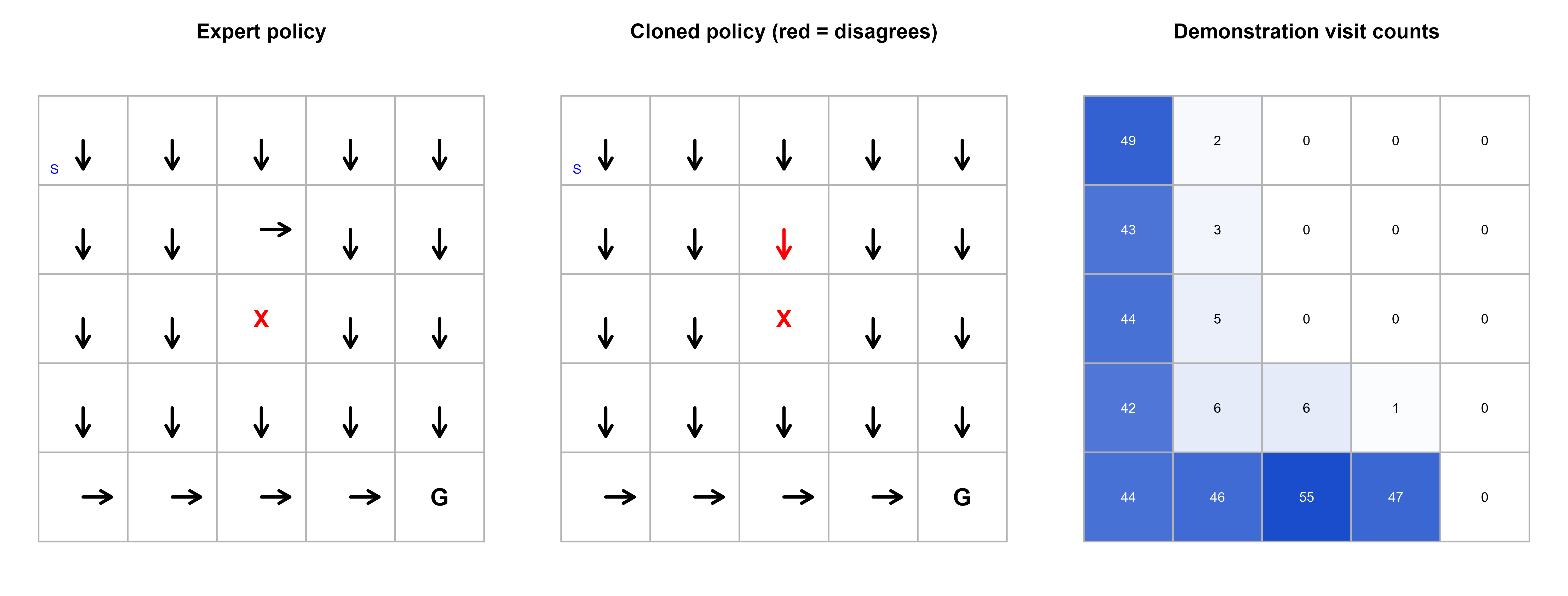
The final exhibit shows the two policies as grids of arrows and marks the cells where the clone disagrees with the expert. The disagreements concentrate away from the expert’s well traveled route, exactly where the demonstration data is thin.
Figure 60.1 shows the expert policy, the cloned policy, and the per cell visitation counts from the demonstrations. Cells the expert visits often are cloned correctly; sparsely visited cells are where the clone’s arrows diverge, which is the visual form of the distribution shift argument.
Show code
# Arrow directions for plottingarrow_dx<-c(up =0, down =0, left =-1, right =1)arrow_dy<-c(up =1, down =-1, left =0, right =0)# Demonstration visitation counts per statevisit_counts<-tabulate(demo_states, nbins =n_states)draw_policy<-function(policy, title, compare=NULL){plot(NA, xlim =c(0.5, grid_n+0.5), ylim =c(0.5, grid_n+0.5), xlab ="", ylab ="", axes =FALSE, main =title, asp =1)for(sin1:n_states){rc<-to_rc(s)x<-rc["col"]; y<-grid_n-rc["row"]+1rect(x-0.5, y-0.5, x+0.5, y+0.5, border ="grey70")if(s==goal_state){text(x, y, "G", cex =1.4, font =2); next}if(s==trap_state){text(x, y, "X", cex =1.4, font =2, col ="red"); next}a<-actions[policy[s]]col<-if(!is.null(compare)&&policy[s]!=compare[s])"red"else"black"arrows(x, y, x+0.32*arrow_dx[a], y+0.32*arrow_dy[a], length =0.08, lwd =2, col =col)if(s==start_state)text(x-0.32, y-0.32, "S", cex =0.8, col ="blue")}}draw_heat<-function(counts, title){plot(NA, xlim =c(0.5, grid_n+0.5), ylim =c(0.5, grid_n+0.5), xlab ="", ylab ="", axes =FALSE, main =title, asp =1)mx<-max(counts)for(sin1:n_states){rc<-to_rc(s)x<-rc["col"]; y<-grid_n-rc["row"]+1shade<-if(mx>0)counts[s]/mxelse0rect(x-0.5, y-0.5, x+0.5, y+0.5, col =rgb(0.1, 0.3, 0.8, alpha =shade), border ="grey70")text(x, y, counts[s], cex =0.8, col =if(shade>0.5)"white"else"black")}}par(mfrow =c(1, 3), mar =c(1, 1, 3, 1))draw_policy(expert_policy, "Expert policy")draw_policy(clone_policy, "Cloned policy (red = disagrees)", compare =expert_policy)draw_heat(visit_counts, "Demonstration visit counts")
Figure 60.1: Left and center: expert and cloned policies as arrows on the 5x5 grid (G = goal, X = trap, S = start), with red arrows marking cells where the clone disagrees with the expert. Right: how often each cell appears in the demonstrations. Disagreements cluster in rarely demonstrated cells, illustrating compounding error.
Note
The exact numbers depend on the random seed, the exploration rate during data collection, and the classifier. The qualitative lesson is robust and is the point of the demo: a clone with high action accuracy still loses task performance, and the losses concentrate exactly where the demonstrations are sparse. Try lowering n_demo_eps to make the data sparser and watch the clone’s success rate fall further; raise it and the gap shrinks.
60.8 Practical guidance and pitfalls
A few hard won lessons for applying these methods.
Measure task performance, not action accuracy. The single most common mistake is to validate a cloned policy by its classification accuracy on held out demonstrations. As the demo shows, that number can be excellent while the policy fails the task. Always evaluate by rolling out the policy and scoring the actual objective.
Demonstrations must cover recovery, not just success. Experts naturally demonstrate the easy, on path states and almost never the awkward off path ones. Deliberately collect recovery data (perturb the system and record the expert’s correction) or use DAgger so the learner’s own mistakes get labeled.
Prefer DAgger when the expert is queryable. If you can ask the expert for the right action on new states (a human labeler, a slow planner, or a privileged simulator), DAgger’s linear error bound is a large practical improvement over cloning’s quadratic one.
Watch out for non Markov experts and hidden state. Humans act on information not in the recorded state (mirrors, intent, what they saw a second ago). If the state given to the learner omits what the expert used, no method can recover the mapping, and the clone will look erratic. Enrich the state or add history.
IRL needs a good feature map (or a flexible reward model). Linear IRL is only as good as \(\phi(s)\). If the features cannot express the true reward, feature matching converges to the wrong behavior. Deep reward models relax this but demand far more data and care.
Causal confusion is a real failure mode. A clone can latch onto a feature that correlates with the expert action in the data but is not its cause (the classic example: an indicator light that turns on because the expert braked, which the clone then uses to decide to brake). More expert data does not fix it; interventions or DAgger style on policy data do.
Use imitation as a warm start, then fine tune with RL. In practice the strongest pipeline clones first to get a competent initial policy cheaply, then improves it with RL against a real or learned reward, which is exactly the supervised fine tuning then RLHF recipe used for aligning language models.
Warning
A cloned policy is only ever as good as its demonstrations and cannot exceed the expert. If the expert is mediocre, the clone is mediocre. To surpass the expert you need a reward signal, through IRL plus RL or through RL fine tuning, because only a reward tells the agent that some unseen behavior is better than what the expert showed.
60.9 Further reading
Ng and Russell (2000), “Algorithms for Inverse Reinforcement Learning,” the paper that framed the IRL problem and its ambiguity.
Abbeel and Ng (2004), “Apprenticeship Learning via Inverse Reinforcement Learning,” which introduced feature expectation matching and the maximum margin formulation.
Ratliff, Bagnell, and Zinkevich (2006), “Maximum Margin Planning,” a structured prediction view of imitation.
Ziebart, Maas, Bagnell, and Dey (2008), “Maximum Entropy Inverse Reinforcement Learning,” the probabilistic formulation that handles suboptimal experts.
Ross and Bagnell (2010), “Efficient Reductions for Imitation Learning,” which established the compounding error bound for behavioral cloning.
Ross, Gordon, and Bagnell (2011), “A Reduction of Imitation Learning and Structured Prediction to No-Regret Online Learning,” the DAgger paper.
Ho and Ermon (2016), “Generative Adversarial Imitation Learning,” which connected IRL to adversarial training and scaled it to high dimensional control.
Osa, Pajarinen, Neumann, Bagnell, Abbeel, and Peters (2018), “An Algorithmic Perspective on Imitation Learning,” a thorough survey of the field.
Sutton and Barto (2018), “Reinforcement Learning: An Introduction” (2nd ed.), for the MDP and RL background this chapter assumes.
Source Code
# Imitation Learning and Inverse Reinforcement Learning {#sec-imitation-inverse-rl}```{r}#| include: falsesource("_common.R")```Suppose you want a system to drive a car, fold a shirt, or write a polite reply, and you have something better than a reward function: you have an expert who already knows how to do the task. Watching a skilled driver is far more informative than handing a robot a steering wheel and a scalar reward, then waiting for it to crash a few thousand times before it stumbles onto good behavior. Imitation learning is the family of methods that turns recorded expert behavior into a policy, and it is often the fastest path from "I have demonstrations" to "I have a working agent."The reinforcement learning chapters (@sec-rl-foundations) assume you could write down a reward function and let an agent discover good behavior through trial and error. That assumption breaks in two common situations. First, the reward is genuinely hard to specify: what numeric reward captures "drive like a careful human"? Second, trial and error is expensive or dangerous: you cannot let a self driving prototype explore by colliding with pedestrians. In both cases you usually do have examples of an expert doing the task well. Imitation learning and inverse reinforcement learning (IRL) are the two main ways to exploit those examples.::: {.callout-tip title="Intuition"}Reinforcement learning answers "what should I do to maximize this reward?" Imitation learning answers a different question: "what would the expert do here?" You replace the reward signal with demonstrations and try to reproduce the behavior that produced them.:::The two approaches in this chapter differ in what they try to copy. Behavioral cloning copies the expert's actions directly: it treats the demonstrations as a labeled dataset and fits a classifier or regressor from states to actions. Inverse reinforcement learning copies the expert's intent: it assumes the expert is optimizing some unknown reward function and tries to recover that reward, after which standard RL produces a policy. Cloning is simple and supervised; IRL is harder but generalizes better because a reward is a more portable description of a task than a lookup table of moves.By the end of the chapter you will understand behavioral cloning and why it suffers from compounding errors, the DAgger algorithm that fixes the compounding problem by querying the expert on the learner's own mistakes, the inverse RL problem and its built in ambiguity, the apprenticeship learning formulation based on feature expectations, and how all of this relates to ordinary RL. A fully runnable base R demonstration clones an expert policy on a small gridworld and measures how far the imitator falls short of the expert, exposing the compounding error problem in numbers you can reproduce.## Where imitation learning fitsThe setup is a Markov decision process (MDP) $(\mathcal{S}, \mathcal{A}, P, R, \gamma)$ exactly as in the reinforcement learning chapters, with one change: the reward $R$ is unknown or unused. The notation throughout is: $\mathcal{S}$ is the set of states, $\mathcal{A}$ the set of actions, $P(s' \mid s, a)$ the transition probability of landing in state $s'$ after action $a$ in state $s$, $\gamma \in [0,1)$ a discount factor, and $\pi(a \mid s)$ a policy mapping states to a distribution over actions.Instead of a reward, you are given a dataset of demonstrations produced by an expert policy $\pi_E$:$$\mathcal{D} = \{ (s_1, a_1), (s_2, a_2), \dots, (s_N, a_N) \},$$a collection of state action pairs sampled from trajectories the expert generated. The goal is to recover a policy $\hat\pi$ that behaves like $\pi_E$.::: {.callout-tip title="When to use this"}Reach for imitation learning when you have demonstrations of good behavior and either the reward is hard to specify or exploration is costly or unsafe. If you can write a clean reward and exploration is cheap, plain RL is simpler. If you have demonstrations but also want to keep improving past the expert, combine imitation as a warm start with RL fine tuning.:::A quick map of the three methods covered here, before the details:- Behavioral cloning: supervised learning from $(s, a)$ pairs. Cheapest, but errors compound on states the expert never visited.- DAgger (dataset aggregation): iterative behavioral cloning that collects new data on states the learner actually reaches, then asks the expert to label them. Fixes compounding errors at the cost of repeated expert access.- Inverse RL and apprenticeship learning: recover a reward (or match feature expectations) rather than copy actions. More work, better generalization, and the output is a reusable reward.## Behavioral cloningBehavioral cloning is the most direct idea imaginable: treat the demonstrations as a supervised dataset, with the state $s$ as the input and the expert action $a$ as the label, and fit a model. If actions are discrete you fit a classifier; if continuous, a regressor. The cloned policy is$$\hat\pi = \arg\min_{\pi} \; \frac{1}{N} \sum_{i=1}^{N} \ell\big(\pi(s_i), a_i\big),$$where $\ell$ is a supervised loss, for example cross entropy for discrete actions or squared error for continuous ones. That is the entire method. Any classifier you already know (logistic regression, a tree, a neural network, k nearest neighbors) is a valid policy class.::: {.callout-important title="Key idea"}Behavioral cloning reduces sequential decision making to a single supervised learning problem. Every tool, intuition, and diagnostic you have for classification transfers directly. This is why it is almost always the first thing to try.:::The catch is subtle and important. Supervised learning assumes the training and test inputs come from the same distribution. In a sequential task that assumption fails, because the states the learner visits depend on the actions the learner takes. If the cloned policy makes a small mistake, it nudges the system into a state slightly different from anything the expert demonstrated. The classifier was never trained there, so it makes a larger mistake, which pushes the system even further off the demonstrated distribution. Errors feed on themselves.### The compounding error problemMake this precise. Let the learner $\hat\pi$ disagree with the expert with probability at most $\epsilon$ on states drawn from the expert's own visitation distribution:$$\mathbb{E}_{s \sim d_{\pi_E}} \big[ \mathbf{1}\{ \hat\pi(s) \neq \pi_E(s) \} \big] \le \epsilon,$$where $d_{\pi_E}$ is the distribution of states the expert visits and $\mathbf{1}\{\cdot\}$ is the indicator function. This is exactly the test error of the classifier. The trouble is that once the learner makes one mistake, the subsequent states are no longer drawn from $d_{\pi_E}$ but from $d_{\hat\pi}$, the learner's own (worse) visitation distribution.A classic result of Ross and Bagnell (2010) bounds the cost of this drift. If the per step error is $\epsilon$ and the task lasts $T$ steps, the expected extra cost of the cloned policy relative to the expert grows like$$J(\hat\pi) - J(\pi_E) \; \le \; O\big(T^2 \epsilon\big),$$ {#eq-imitation-inverse-rl-bc-bound}where $J(\pi)$ is the total expected cost over a horizon of $T$ steps. The quadratic $T^2$ is the signature of compounding error. Contrast this with the linear $O(T\epsilon)$ you would get if the state distribution did not shift. Over a long horizon, even a tiny supervised error can blow up.#### Deriving the quadratic bound {#sec-imitation-inverse-rl-bc-derivation}It is worth seeing where the $T^2$ comes from, because the derivation pinpoints exactly which step fails and motivates the DAgger fix. Work with costs (so smaller is better) and a finite horizon $T$. Let $c(s,a) \in [0,1]$ be a per step cost, let $d_\pi^t$ denote the distribution of states visited at time $t$ under policy $\pi$, and define the total cost$$J(\pi) = \sum_{t=1}^{T} \mathbb{E}_{s \sim d_\pi^t}\big[\, c(s, \pi(s)) \,\big].$$Assume the supervised step controls the per step disagreement under the expert's own visitation distribution: at every $t$,$$\mathbb{E}_{s \sim d_{\pi_E}^t}\big[\, \mathbf{1}\{\hat\pi(s) \neq \pi_E(s)\} \,\big] \le \epsilon.$$ {#eq-imitation-inverse-rl-bc-assumption}The argument has two parts: bound how fast the learner's state distribution drifts from the expert's, then turn that drift into a cost gap.Step one, distribution drift. Couple the two trajectories: run the expert and the learner from the same start with shared randomness, and let $p_t$ be the probability that they have made at least one disagreeing action by time $t$. As long as no disagreement has occurred, the two systems occupy identical states, so the chance of a fresh disagreement at step $t$ is at most $\epsilon$ by @eq-imitation-inverse-rl-bc-assumption. Hence $p_t \le p_{t-1} + \epsilon$, and with $p_0 = 0$ we get $p_t \le t\epsilon$. The total variation distance between the two state distributions at time $t$ is bounded by this coupling failure probability,$$\big\| d_{\hat\pi}^t - d_{\pi_E}^t \big\|_1 \le 2\, p_t \le 2 t \epsilon .$$ {#eq-imitation-inverse-rl-bc-tv}Step two, cost gap. Decompose the learner's cost at each step by comparing it to the expert on the expert's distribution, then paying for the distribution shift. Since costs lie in $[0,1]$,$$\mathbb{E}_{s \sim d_{\hat\pi}^t}\big[ c(s, \hat\pi(s)) \big]\;\le\; \underbrace{\mathbb{E}_{s \sim d_{\pi_E}^t}\big[ c(s, \hat\pi(s)) \big]}_{\text{learner on expert states}}\;+\; \big\| d_{\hat\pi}^t - d_{\pi_E}^t \big\|_1 .$$On the expert's states the learner matches the expert except on an $\epsilon$ fraction where the cost can differ by at most $1$, so $\mathbb{E}_{s \sim d_{\pi_E}^t}[ c(s, \hat\pi(s)) ] \le \mathbb{E}_{s \sim d_{\pi_E}^t}[ c(s, \pi_E(s)) ] + \epsilon$. Combining with @eq-imitation-inverse-rl-bc-tv,$$\mathbb{E}_{s \sim d_{\hat\pi}^t}\big[ c(s, \hat\pi(s)) \big]\;\le\; \mathbb{E}_{s \sim d_{\pi_E}^t}\big[ c(s, \pi_E(s)) \big] + \epsilon + 2 t \epsilon .$$Summing over $t = 1, \dots, T$ and cancelling the matched expert cost gives$$J(\hat\pi) - J(\pi_E) \;\le\; \sum_{t=1}^{T} \big( \epsilon + 2 t \epsilon \big)\;=\; T\epsilon + 2\epsilon \tfrac{T(T+1)}{2} \;=\; O\big(T^2 \epsilon\big),$$which is @eq-imitation-inverse-rl-bc-bound. The quadratic is now transparent: one factor of $T$ is the horizon (you pay the per step error $T$ times), and the second factor is the drift, because the drift itself accumulates linearly in $t$ (@eq-imitation-inverse-rl-bc-tv). The fatal step is the appeal to @eq-imitation-inverse-rl-bc-assumption, an error guarantee under $d_{\pi_E}$, when the learner is actually evaluated under $d_{\hat\pi}$. Any method that instead controls the error under the learner's own distribution removes the second factor of $T$, which is precisely what DAgger does.::: {.callout-warning}The $T^2$ blow up is not a pessimistic worst case curiosity; it is what you actually observe. A behavioral cloning agent can score 99 percent action accuracy on a held out demonstration set and still fail the task badly, because the 1 percent of mistakes land it in unfamiliar states where its accuracy is far worse. Action accuracy on expert data is a misleading proxy for task performance.:::::: {.callout-tip title="Intuition"}Think of walking a tightrope by copying a video of an acrobat. Each frame you imitate almost perfectly. But the tiny errors push you slightly off balance into poses the acrobat never struck, and the video has no advice for those poses. The further you drift, the less the demonstrations help, and you fall. The expert's data covers only the narrow ridge of states the expert visited.:::### Practical remedies short of new algorithmsSeveral cheap fixes reduce, though do not eliminate, the compounding problem:- Collect more demonstrations, especially recoveries: deliberately have the expert demonstrate getting back on track from off distribution states (in driving datasets, this is recorded by perturbing the car and recording the human's correction).- Add noise to the expert during data collection so the demonstrations naturally cover states near the ideal path, giving the classifier examples of recovery.- Regularize and use a policy class that degrades gracefully, so off distribution predictions are reasonable rather than wild.- Predict action sequences or use history, which can smooth out single step errors.The principled fix, however, is to change what data you train on, which is what DAgger does.## DAgger: dataset aggregationDAgger (Ross, Gordon, and Bagnell, 2011) attacks the distribution mismatch at its root. The problem is that the learner is trained on the expert's states but tested on its own states. DAgger closes that gap by training on the learner's own states, with labels supplied by the expert.The algorithm is iterative. Start with a behavioral cloning policy. Then repeat: roll out the current learner to collect the states it actually visits, ask the expert what it would have done in each of those states, add these freshly labeled pairs to the dataset, and refit the policy on the aggregated dataset. Each round, the training distribution moves closer to the distribution the learner induces, so the classifier is trained exactly where it will be tested.A common refinement mixes the expert and learner during rollouts so that early iterations, when the learner is poor, do not wander uselessly far. Let $\beta_i$ be the probability of using the expert action at iteration $i$, with $\beta_i \to 0$. The rollout policy is$$\pi_i = \beta_i\, \pi_E + (1 - \beta_i)\, \hat\pi_i .$$A typical schedule is $\beta_i = p^{i}$ for some $p < 1$, or simply $\beta_1 = 1$ (pure expert on the first pass, which recovers ordinary behavioral cloning) and $\beta_i = 0$ thereafter.The payoff is a better bound. Under DAgger the performance gap becomes linear in the horizon,$$J(\hat\pi) - J(\pi_E) \; \le \; O(T \epsilon),$$ {#eq-imitation-inverse-rl-dagger-bound}removing one factor of $T$ compared with plain cloning. The intuition is that the learner is never tested on states it was not trained on, so a single mistake no longer cascades unboundedly.### Why DAgger earns the linear boundThe improvement is not magic, and seeing the mechanism clarifies both what DAgger guarantees and what it assumes. The key change is the distribution under which the supervised error is controlled. Let $\bar d = \frac1T \sum_{t=1}^T d_{\hat\pi}^t$ be the learner's own time averaged state distribution, the distribution DAgger actually trains on once $\beta_i \to 0$. Suppose the aggregated classifier achieves$$\mathbb{E}_{s \sim \bar d}\big[\, \mathbf{1}\{\hat\pi(s) \neq \pi_E(s)\} \,\big] \le \epsilon ,$$ {#eq-imitation-inverse-rl-dagger-assumption}which is exactly the held out error of the final model measured on rollouts of the learner, the quantity DAgger drives down by aggregation. Now decompose the cost gap one step at a time. Write the per step disadvantage of taking the learner's action versus the expert's action and following the expert afterward; because the learner and expert states already coincide in this accounting (both costs are evaluated under $d_{\hat\pi}^t$), there is no second distribution shift term to pay. Each disagreement, occurring on at most an $\epsilon$ fraction of states by @eq-imitation-inverse-rl-dagger-assumption, costs at most $1$ (or a problem dependent constant $u$, the maximum extra cost of a single wrong action). Summing the $T$ steps,$$J(\hat\pi) - J(\pi_E) \;\le\; \sum_{t=1}^{T} u \cdot \mathbb{E}_{s \sim d_{\hat\pi}^t}\big[ \mathbf{1}\{\hat\pi(s) \neq \pi_E(s)\} \big] \;\le\; u\, T \epsilon \;=\; O(T\epsilon),$$which is @eq-imitation-inverse-rl-dagger-bound. Compared with the cloning derivation, the missing term is the $\sum_t 2t\epsilon$ drift penalty: it vanishes because @eq-imitation-inverse-rl-dagger-assumption already measures error on $d_{\hat\pi}$, so no coupling argument is needed and the second factor of $T$ never appears.Two caveats make this honest. First, DAgger is an online learning procedure, and @eq-imitation-inverse-rl-dagger-assumption is achievable only in an average sense: the no regret analysis of Ross, Gordon, and Bagnell (2011) shows the best policy in the aggregated sequence attains error $\epsilon + O(1/N)$ after $N$ iterations, where the $O(1/N)$ is the average regret of the online learner. Second, the bound assumes the expert can be queried on the off distribution states the learner visits, which is the practical price for the better rate, as the callout below notes.::: {.callout-note}DAgger's cost is repeated access to the expert. It assumes you can query the expert for the correct action on arbitrary states the learner visits, including awkward ones. That is reasonable when the expert is a human labeler or a slow but available planner, and unreasonable when the expert is a one time recorded dataset with no way to ask follow up questions. The right method depends on whether your expert is queryable or only logged.:::## Inverse reinforcement learningBehavioral cloning and DAgger copy actions. Inverse reinforcement learning copies intent. The premise is that the expert is (approximately) optimal for some reward function $R$ that you do not know, and that recovering $R$ is more useful than recovering the actions, because a reward generalizes to new states, new dynamics, and even new agents in a way a memorized action map cannot.Formally, given demonstrations from an expert assumed optimal under an unknown reward $R^\star$, find a reward $\hat R$ such that the optimal policy for $\hat R$ matches the expert. The reward is usually modeled as a linear combination of state features $\phi(s) \in \mathbb{R}^k$:$$R(s) = w^\top \phi(s),$$where $w \in \mathbb{R}^k$ is the weight vector to be estimated and $\phi(s)$ is a known feature map (for example, indicators for terrain type, distance to a goal, proximity to hazards).### The ambiguity problemIRL is fundamentally ill posed. Many reward functions make the same behavior optimal, and some make every behavior optimal. The reward $R(s) = 0$ everywhere makes any policy optimal, so it trivially explains any demonstration. Scaling a reward by a positive constant, or adding a constant, does not change the optimal policy either. So the raw question "which reward did the expert optimize?" has no unique answer.::: {.callout-important title="Key idea"}IRL does not have a single correct reward, so every IRL method needs an extra principle to pick one reward among the many that explain the data. The choice of that principle is what distinguishes the major algorithms: maximum margin (Abbeel and Ng, 2004), maximum entropy (Ziebart et al., 2008), and adversarial matching (Ho and Ermon, 2016).:::### Apprenticeship learning via feature matchingAbbeel and Ng (2004) sidestep the ambiguity with a clever observation. If the reward is linear, $R(s) = w^\top \phi(s)$, then the expected discounted return of a policy depends only on its expected discounted feature counts, called feature expectations:$$\mu(\pi) = \mathbb{E}\!\left[ \sum_{t=0}^{\infty} \gamma^t \, \phi(s_t) \;\Big|\; \pi \right] \in \mathbb{R}^k .$$The value of a policy is then simply $J(\pi) = w^\top \mu(\pi)$. To see this, expand the value definition and use linearity of expectation,$$J(\pi) = \mathbb{E}\!\left[ \sum_{t=0}^\infty \gamma^t R(s_t) \,\Big|\, \pi \right]= \mathbb{E}\!\left[ \sum_{t=0}^\infty \gamma^t\, w^\top \phi(s_t) \,\Big|\, \pi \right]= w^\top \, \mathbb{E}\!\left[ \sum_{t=0}^\infty \gamma^t \phi(s_t) \,\Big|\, \pi \right]= w^\top \mu(\pi),$$where pulling the constant $w$ out of the expectation is the only algebraic move and it relies entirely on the reward being linear in $\phi$. The key consequence: if a learner's feature expectations match the expert's, $\mu(\hat\pi) = \mu(\pi_E)$, then the learner achieves the same value as the expert for every reward in the linear class, whatever the true $w$ turns out to be. Concretely, for any $\|w\|_2 \le 1$,$$\big| J(\hat\pi) - J(\pi_E) \big| = \big| w^\top (\mu(\hat\pi) - \mu(\pi_E)) \big|\le \|w\|_2 \, \|\mu(\hat\pi) - \mu(\pi_E)\|_2 \le \varepsilon ,$$by Cauchy to Schwarz, so matching feature expectations to within $\varepsilon$ bounds the value gap by $\varepsilon$ under the worst case reward in the class. You do not need to identify $w$ at all; you only need to match feature expectations. Note also that $\mu(\pi_E)$ is estimated from the $m$ demonstrated trajectories by the empirical average $\hat\mu_E = \frac1m \sum_{i=1}^m \sum_t \gamma^t \phi(s_t^{(i)})$, whose feature counts are bounded in $[0, \frac{1}{1-\gamma}]$ per coordinate, so a Hoeffding argument gives estimation error $\|\hat\mu_E - \mu(\pi_E)\|_\infty = O\big( \frac{1}{1-\gamma} \sqrt{\log(k/\delta)/m} \big)$ with probability $1-\delta$; this is the sample complexity of the expert side.Apprenticeship learning turns this into an iterative game. At each round you find the reward weights that most favor the expert over the current learner (the maximum margin step), then run RL to compute the best policy for that reward, and repeat until the learner's feature expectations are within $\varepsilon$ of the expert's:$$\| \mu(\hat\pi) - \mu(\pi_E) \|_2 \le \varepsilon .$$The maximum margin subproblem is$$\max_{w:\, \|w\|_2 \le 1} \; \min_{j} \; w^\top \big( \mu(\pi_E) - \mu(\pi_j) \big),$$which seeks the reward direction along which the expert most outperforms every previously found policy $\pi_j$. This is the same structure as a support vector machine (@sec-svm), and it gives the method its "maximum margin" name.#### Convergence of the projection algorithmAbbeel and Ng also give a simpler variant, the projection algorithm, whose convergence is easy to state and proves the procedure terminates. It maintains an estimate $\bar\mu_j$ of the expert's feature expectation, initialized at $\bar\mu_0 = \mu(\pi_0)$ for an arbitrary first policy. At iteration $j$ it sets the reward direction to $w_{j} = \mu(\pi_E) - \bar\mu_{j-1}$, computes the RL optimal policy $\pi_j$ for that reward, obtaining $\mu(\pi_j)$, and then orthogonally projects $\mu(\pi_E)$ onto the line through $\bar\mu_{j-1}$ and $\mu(\pi_j)$ to update $\bar\mu_j$. Because each step is an orthogonal projection toward $\mu(\pi_E)$ within the convex hull of the discovered $\mu(\pi_j)$, the distance contracts geometrically and one can show$$\big\| \mu(\pi_E) - \bar\mu_j \big\|_2 \;\le\; \frac{k_{\max}}{(1-\gamma)\sqrt{j}} ,$$where $k_{\max} = \max_s \|\phi(s)\|_2$ bounds the feature norm. Hence after$$j = O\!\left( \frac{k_{\max}^2}{(1-\gamma)^2\, \varepsilon^2} \right)$$iterations the feature expectations are within $\varepsilon$, each iteration costing one full RL solve. The output is a mixture policy over the $\{\pi_j\}$ (randomize once at the start over which $\pi_j$ to follow for the whole episode); this stochastic mixture, not any single $\pi_j$, is what attains $\mu(\hat\pi) \approx \mu(\pi_E)$. This is a notable subtlety: feature matching guarantees the value of a mixture of deterministic policies, which is generally not realizable by any single deterministic policy.::: {.callout-warning}Feature matching guarantees only that $\hat\pi$ matches the expert's value under the assumed linear reward class. If the true reward is not linear in $\phi$, matching $\mu$ does not match behavior, and the recovered policy can differ markedly from the expert while sharing feature counts. This is the apprenticeship analogue of model misspecification, and it is why the choice of $\phi$ dominates the method's success.:::### Maximum entropy IRL and modern variantsMaximum entropy IRL (Ziebart et al., 2008) resolves the ambiguity differently and more robustly. Among all trajectory distributions that match the expert's feature expectations, it picks the one with maximum entropy, which is the least committed distribution consistent with the evidence. This yields a probabilistic model in which trajectories are exponentially more likely as their return increases:$$p(\tau) \; \propto \; \exp\!\big( w^\top \phi(\tau) \big),$$ {#eq-imitation-inverse-rl-maxent-form}where $\phi(\tau) = \sum_t \gamma^t \phi(s_t)$ is the trajectory feature count. The weights $w$ are then fit by maximum likelihood on the demonstrated trajectories, which handles suboptimal or noisy experts gracefully because it assigns nonzero probability to imperfect behavior.#### Deriving the exponential formThe exponential model in @eq-imitation-inverse-rl-maxent-form is not an assumption; it is the unique solution of the maximum entropy program, and deriving it shows where $w$ enters. The principle is: among all distributions $p$ over trajectories that reproduce the empirically observed feature expectations $\tilde\mu = \mathbb{E}_{\tilde p}[\phi(\tau)]$, choose the one of maximum (differential) entropy. That is the constrained problem$$\max_{p} \; -\sum_\tau p(\tau) \log p(\tau)\quad \text{s.t.} \quad \sum_\tau p(\tau)\,\phi(\tau) = \tilde\mu, \;\; \sum_\tau p(\tau) = 1 .$$Form the Lagrangian with multipliers $w \in \mathbb{R}^k$ for the feature constraints and $\lambda$ for normalization,$$\mathcal{L} = -\sum_\tau p(\tau)\log p(\tau) + w^\top\!\Big(\sum_\tau p(\tau)\phi(\tau) - \tilde\mu\Big) + \lambda\Big(\sum_\tau p(\tau) - 1\Big).$$Differentiate with respect to a single $p(\tau)$ and set to zero,$$\frac{\partial \mathcal{L}}{\partial p(\tau)} = -\log p(\tau) - 1 + w^\top \phi(\tau) + \lambda = 0\;\;\Longrightarrow\;\;p(\tau) = \exp\!\big( w^\top \phi(\tau) + \lambda - 1 \big).$$Absorbing the constant into a normalizer $Z(w) = \sum_\tau \exp(w^\top \phi(\tau))$ enforced by $\sum_\tau p(\tau) = 1$ gives exactly @eq-imitation-inverse-rl-maxent-form, $p(\tau) = \frac{1}{Z(w)}\exp(w^\top \phi(\tau))$. The Lagrange multipliers $w$ on the feature constraints are precisely the reward weights, so the maximum entropy distribution and the linear reward fall out of the same variational problem. (With stochastic dynamics one conditions on $P(s'\mid s,a)$ and the clean form holds in the deterministic case; Ziebart et al. give the dynamics aware correction.)#### The maximum likelihood gradientFitting $w$ by maximum likelihood on the $m$ demonstrated trajectories means maximizing $\mathcal{L}(w) = \frac1m \sum_{i=1}^m \log p(\tau_i) = \frac1m\sum_i w^\top \phi(\tau_i) - \log Z(w)$. The gradient of the log normalizer is the model's expected feature count, since$$\nabla_w \log Z(w) = \frac{1}{Z(w)} \sum_\tau \exp(w^\top\phi(\tau))\,\phi(\tau) = \mathbb{E}_{\tau \sim p_w}[\phi(\tau)] = \mu(\pi_w),$$a standard exponential family identity (the log partition function generates the moments). Therefore$$\nabla_w \mathcal{L}(w) = \underbrace{\tfrac1m\textstyle\sum_i \phi(\tau_i)}_{\hat\mu_E} - \underbrace{\mu(\pi_w)}_{\text{model's feature count}} = \hat\mu_E - \mu(\pi_w).$$ {#eq-imitation-inverse-rl-maxent-grad}This is the defining result of MaxEnt IRL: the likelihood gradient is the difference between the expert's empirical feature expectations and the feature expectations of the current maximum entropy policy. Gradient ascent therefore drives $\mu(\pi_w) \to \hat\mu_E$, recovering feature matching as the stationary condition $\nabla_w\mathcal{L} = 0$, but now derived from a probabilistic likelihood rather than imposed by a margin. Computing $\mu(\pi_w)$ requires the expected state visitation under the current soft optimal policy, obtained by a forward backward dynamic program over the MDP (the soft value iteration that replaces the hard $\max$ with a log sum exp), which is the per iteration cost of the method.The gradient identity @eq-imitation-inverse-rl-maxent-grad is easy to confirm numerically on a small trajectory set: the analytic gradient $\hat\mu_E - \mu(\pi_w)$ should match a finite difference of the log likelihood.```{r imitation-inverse-rl-maxent-check}set.seed(1)# A tiny universe of candidate trajectories, each with a 2-dim feature count.Phi <-matrix(c(2, 0, 1, 1, 0, 2, 1, 0, 0, 1), ncol =2, byrow =TRUE)demo <-c(1, 1, 2) # observed (expert) trajectory indicesmu_hat <-colMeans(Phi[demo, , drop =FALSE]) # empirical expert feature countloglik <-function(w) { # MaxEnt log-likelihood at weights w s <- Phi %*% wmean(Phi[demo, , drop =FALSE] %*% w) - (max(s) +log(sum(exp(s -max(s)))))}grad_analytic <-function(w) { # mu_hat - E_{p_w}[phi] p <-exp(Phi %*% w -max(Phi %*% w)); p <- p /sum(p)as.numeric(mu_hat -t(Phi) %*% p)}w0 <-c(0.3, -0.2); eps <-1e-6grad_num <-c((loglik(w0 +c(eps, 0)) -loglik(w0 -c(eps, 0))) / (2* eps), (loglik(w0 +c(0, eps)) -loglik(w0 -c(0, eps))) / (2* eps))cat("analytic:", round(grad_analytic(w0), 6), "\n")cat("numeric :", round(grad_num, 6), "\n")cat("max abs difference:", max(abs(grad_analytic(w0) - grad_num)), "\n")```The analytic and numerical gradients agree to within rounding, confirming that the likelihood gradient is exactly the feature expectation mismatch.Two threads grew from this. Adversarial imitation, exemplified by generative adversarial imitation learning (GAIL, Ho and Ermon, 2016), trains a discriminator to tell expert trajectories from learner trajectories and uses it as a reward signal, connecting IRL to generative adversarial networks (@sec-generative-models) and skipping the explicit reward recovery. Deep maximum entropy IRL replaces the linear $w^\top \phi$ with a neural network reward. Both push the same idea to high dimensional problems.## Comparing the approaches@tbl-imitation-inverse-rl-methods lays out the four methods side by side: what each one outputs, what it assumes about access to the expert and the environment, how it handles the distribution shift problem, and when it is a sensible default.| Property | Behavioral cloning | DAgger | Apprenticeship / max margin IRL | MaxEnt / adversarial IRL ||---|---|---|---|---|| What it learns | Policy (state to action map) | Policy, refined iteratively | Reward weights, then a policy | Reward (or implicit reward), then a policy || Expert access | Logged data only | Interactive queries each round | Logged data, but needs RL solves | Logged data, plus RL or rollouts || Needs environment model or simulator | No | Yes (to roll out the learner) | Yes (RL inner loop) | Yes (RL or sampling inner loop) || Distribution shift | Compounding, $O(T^2\epsilon)$ | Mitigated, $O(T\epsilon)$ | Addressed via feature matching | Addressed via distribution matching || Handles suboptimal experts | Poorly | Poorly | Poorly | Well (probabilistic) || Generalizes to new dynamics | No | No | Yes (reward transfers) | Yes (reward transfers) || Cost and complexity | Lowest | Low to medium | High | High || Good default for | First attempt, abundant data | Queryable expert, drift is the problem | Want a reusable reward, linear features | Noisy experts, high dimensional tasks |: Comparison of imitation learning and inverse reinforcement learning methods across what they output, their assumptions, how they handle distribution shift, and when each is a reasonable default. {#tbl-imitation-inverse-rl-methods}## Relation to reinforcement learningIt helps to see imitation and IRL as two ends of a pipeline that has RL in the middle. Ordinary RL maps a reward to a policy. IRL runs that map backward, from demonstrations to a reward. Apprenticeship learning and adversarial imitation then close the loop, alternating IRL (infer a reward) with RL (optimize it). Behavioral cloning short circuits the whole pipeline by skipping the reward and the dynamics entirely, learning the policy directly with supervised learning.A useful way to remember the relationships:- RL: reward $\to$ policy (forward).- IRL: demonstrations $\to$ reward (inverse), then RL to get a policy.- Behavioral cloning: demonstrations $\to$ policy (supervised, no reward, no dynamics).- Apprenticeship / GAIL: alternate IRL and RL until the learner matches the expert.In modern practice these blend. The reinforcement learning from human feedback (RLHF) used to align large language models (@sec-llms) is essentially IRL followed by RL: a reward model is fit to human preference comparisons (a form of recovering the reward behind expert judgments), then a policy is optimized against that learned reward. Behavioral cloning, under the name supervised fine tuning, is the warm start that precedes it.::: {.callout-tip title="Intuition"}If you only need the agent to act in the same environment it was trained in, copying actions (behavioral cloning) may be enough. If you need it to act well in a new environment, or to keep improving, recover the reward (IRL), because intent transfers where a memorized action map does not.:::## Runnable demo: behavioral cloning on a gridworldTo make the compounding error problem concrete, the rest of the chapter builds a small gridworld, computes an optimal expert policy by value iteration, generates expert demonstrations, clones the policy with a simple classifier, and measures how the imitator's success rate degrades relative to the expert. Everything is base R so that every moving part is visible.The world is a $5 \times 5$ grid. The agent starts in the top left corner and must reach a goal in the bottom right. One cell is a trap. The agent can move up, down, left, or right; bumping into a wall keeps it in place. Reaching the goal gives a large reward, the trap gives a large penalty, and every step costs a little to encourage short paths.### Building the environment and the expertFirst the environment and an exact optimal policy via value iteration. Because the dynamics are known here, the expert is genuinely optimal, which makes it a clean teacher for the cloning experiment.```{r imitation-inverse-rl-setup}set.seed(42)# Gridworld geometrygrid_n <-5n_states <- grid_n * grid_nactions <-c("up", "down", "left", "right")n_act <-length(actions)start_state <-1# top-left (row 1, col 1)goal_state <- n_states # bottom-right (row 5, col 5)trap_state <-13# a cell in the middle (row 3, col 3)# Map a state id to (row, col) and backto_rc <-function(s) c(row = ((s -1) %/% grid_n) +1,col = ((s -1) %% grid_n) +1)to_s <-function(r, c) (r -1) * grid_n + c# Deterministic transition: returns the next state idstep_env <-function(s, a) { rc <-to_rc(s); r <- rc["row"]; c <- rc["col"]if (a =="up") r <-max(1, r -1)if (a =="down") r <-min(grid_n, r +1)if (a =="left") c <-max(1, c -1)if (a =="right") c <-min(grid_n, c +1)as.integer(to_s(r, c))}# Reward for landing in a statereward_of <-function(s) {if (s == goal_state) return(10)if (s == trap_state) return(-10)-0.1# small step cost}is_terminal <-function(s) s == goal_state || s == trap_state# Value iteration to get the optimal expert policygamma <-0.95V <-rep(0, n_states)for (iter in1:500) { V_new <- Vfor (s in1:n_states) {if (is_terminal(s)) { V_new[s] <-reward_of(s); next } q <-sapply(actions, function(a) { s2 <-step_env(s, a)reward_of(s2) + gamma * V[s2] }) V_new[s] <-max(q) }if (max(abs(V_new - V)) <1e-8) { V <- V_new; break } V <- V_new}# Greedy expert policy: best action index per stateexpert_policy <-integer(n_states)for (s in1:n_states) { q <-sapply(actions, function(a) { s2 <-step_env(s, a); reward_of(s2) + gamma * V[s2] }) expert_policy[s] <-which.max(q)}cat("Expert policy (action index per cell, row-major):\n")print(matrix(expert_policy, nrow = grid_n, byrow =TRUE))```### Generating demonstrationsThe expert rolls out from the start to produce state action pairs. To keep the cloning problem interesting (and to mirror how real demonstration data fails to cover the whole space), the expert is mostly greedy but occasionally explores, so the demonstrations cover a realistic but incomplete slice of the state space.```{r imitation-inverse-rl-demos}# Roll out a policy (given as action indices per state) from the start.# epsilon adds exploration so demonstrations are not a single fixed path.rollout <-function(policy, epsilon =0, max_steps =50) { s <- start_state states <-integer(0); acts <-integer(0)for (t in1:max_steps) {if (is_terminal(s)) break a_idx <-if (runif(1) < epsilon) sample.int(n_act, 1) else policy[s] states <-c(states, s); acts <-c(acts, a_idx) s <-step_env(s, actions[a_idx]) }list(states = states, acts = acts, final = s)}# Collect demonstrations from many epsilon-soft expert episodesn_demo_eps <-40demo_states <-integer(0); demo_acts <-integer(0)for (e in1:n_demo_eps) { ro <-rollout(expert_policy, epsilon =0.15) demo_states <-c(demo_states, ro$states) demo_acts <-c(demo_acts, ro$acts)}cat("Collected", length(demo_states), "state-action pairs from", n_demo_eps, "episodes.\n")cat("Distinct states visited in demonstrations:",length(unique(demo_states)), "of", n_states, "\n")```### Cloning the policy with a classifierThe cloned policy is a classifier from state features to the action index. The state features are the one hot encoded row and column, so the classifier has something to generalize from rather than memorizing raw state ids. Base R multinomial logistic regression via repeated binomial fits keeps the demo dependency free; each action gets a one versus rest logistic model, and prediction picks the action with the highest score.```{r imitation-inverse-rl-clone}# Feature map: one-hot row and column for a state -> length 2*grid_n vectorfeatures <-function(s) { rc <-to_rc(s) f_row <-as.numeric(seq_len(grid_n) == rc["row"]) f_col <-as.numeric(seq_len(grid_n) == rc["col"])c(f_row, f_col)}# Build the supervised training matrix from demonstrationsX <-t(sapply(demo_states, features))colnames(X) <-c(paste0("r", 1:grid_n), paste0("c", 1:grid_n))y <- demo_acts# One-vs-rest logistic regression, one model per action present in datapresent_acts <-sort(unique(y))models <-list()for (a in present_acts) { yb <-as.integer(y == a) df <-data.frame(yb = yb, X) models[[as.character(a)]] <-suppressWarnings(glm(yb ~ ., data = df, family =binomial()))}# Cloned policy: predict best action for every state in the gridclone_action <-function(s) { xf <-as.data.frame(t(features(s)))colnames(xf) <-colnames(X) scores <-sapply(present_acts, function(a)suppressWarnings(predict(models[[as.character(a)]], xf, type ="link"))) present_acts[which.max(scores)]}clone_policy <-sapply(1:n_states, clone_action)# Action-matching accuracy on the demonstrated states (the misleading metric)train_pred <-sapply(demo_states, clone_action)bc_action_acc <-mean(train_pred == demo_acts)cat(sprintf("Behavioral cloning action accuracy on demo states: %.1f%%\n",100* bc_action_acc))```### Measuring task performance, not action accuracyAction accuracy on the demonstrated states is the misleading metric warned about earlier. The honest test is task performance: run each policy from the start and check whether it reaches the goal, and with what return. To expose compounding error, we also evaluate from every non terminal start cell, including cells the demonstrations rarely or never covered.```{r imitation-inverse-rl-eval}# Run a deterministic policy from a given start; return success and return.evaluate_from <-function(policy, start, max_steps =50) { s <- start; total <-0; disc <-1for (t in1:max_steps) {if (is_terminal(s)) break s2 <-step_env(s, actions[policy[s]]) total <- total + disc *reward_of(s2) disc <- disc * gamma s <- s2 }list(success = (s == goal_state), ret = total)}# Evaluate both policies from every non-terminal cellcells <-setdiff(1:n_states, c(goal_state, trap_state))expert_succ <-mean(sapply(cells, function(s) evaluate_from(expert_policy, s)$success))clone_succ <-mean(sapply(cells, function(s) evaluate_from(clone_policy, s)$success))expert_ret <-mean(sapply(cells, function(s) evaluate_from(expert_policy, s)$ret))clone_ret <-mean(sapply(cells, function(s) evaluate_from(clone_policy, s)$ret))results <-data.frame(Policy =c("Expert (optimal)", "Behavioral cloning"),SuccessRate =c(expert_succ, clone_succ),MeanReturn =c(expert_ret, clone_ret))print(results)```@tbl-imitation-inverse-rl-results reports the success rate (fraction of start cells from which the policy reaches the goal) and the mean discounted return for the expert and the clone. The clone matches the expert on its action labels yet reaches the goal from fewer starting cells, because once it steps off the demonstrated path it has no reliable guidance, which is the compounding error problem made numeric.```{r tbl-imitation-inverse-rl-results}knitr::kable( results,digits =3,col.names =c("Policy", "Success rate", "Mean discounted return"),caption ="Expert versus behavioral-cloning performance, averaged over every non-terminal start cell. The clone has high action accuracy on demonstrated states but a lower task success rate, the signature of compounding error on states the expert rarely visited.")```### Visualizing where the clone divergesThe final exhibit shows the two policies as grids of arrows and marks the cells where the clone disagrees with the expert. The disagreements concentrate away from the expert's well traveled route, exactly where the demonstration data is thin.@fig-imitation-inverse-rl-policy-map shows the expert policy, the cloned policy, and the per cell visitation counts from the demonstrations. Cells the expert visits often are cloned correctly; sparsely visited cells are where the clone's arrows diverge, which is the visual form of the distribution shift argument.```{r fig-imitation-inverse-rl-policy-map, fig.cap="Left and center: expert and cloned policies as arrows on the 5x5 grid (G = goal, X = trap, S = start), with red arrows marking cells where the clone disagrees with the expert. Right: how often each cell appears in the demonstrations. Disagreements cluster in rarely demonstrated cells, illustrating compounding error.", fig.width=10, fig.height=3.8}# Arrow directions for plottingarrow_dx <-c(up =0, down =0, left =-1, right =1)arrow_dy <-c(up =1, down =-1, left =0, right =0)# Demonstration visitation counts per statevisit_counts <-tabulate(demo_states, nbins = n_states)draw_policy <-function(policy, title, compare =NULL) {plot(NA, xlim =c(0.5, grid_n +0.5), ylim =c(0.5, grid_n +0.5),xlab ="", ylab ="", axes =FALSE, main = title, asp =1)for (s in1:n_states) { rc <-to_rc(s) x <- rc["col"]; y <- grid_n - rc["row"] +1rect(x -0.5, y -0.5, x +0.5, y +0.5, border ="grey70")if (s == goal_state) { text(x, y, "G", cex =1.4, font =2); next }if (s == trap_state) { text(x, y, "X", cex =1.4, font =2, col ="red"); next } a <- actions[policy[s]] col <-if (!is.null(compare) && policy[s] != compare[s]) "red"else"black"arrows(x, y, x +0.32* arrow_dx[a], y +0.32* arrow_dy[a],length =0.08, lwd =2, col = col)if (s == start_state) text(x -0.32, y -0.32, "S", cex =0.8, col ="blue") }}draw_heat <-function(counts, title) {plot(NA, xlim =c(0.5, grid_n +0.5), ylim =c(0.5, grid_n +0.5),xlab ="", ylab ="", axes =FALSE, main = title, asp =1) mx <-max(counts)for (s in1:n_states) { rc <-to_rc(s) x <- rc["col"]; y <- grid_n - rc["row"] +1 shade <-if (mx >0) counts[s] / mx else0rect(x -0.5, y -0.5, x +0.5, y +0.5,col =rgb(0.1, 0.3, 0.8, alpha = shade), border ="grey70")text(x, y, counts[s], cex =0.8,col =if (shade >0.5) "white"else"black") }}par(mfrow =c(1, 3), mar =c(1, 1, 3, 1))draw_policy(expert_policy, "Expert policy")draw_policy(clone_policy, "Cloned policy (red = disagrees)", compare = expert_policy)draw_heat(visit_counts, "Demonstration visit counts")```::: {.callout-note}The exact numbers depend on the random seed, the exploration rate during data collection, and the classifier. The qualitative lesson is robust and is the point of the demo: a clone with high action accuracy still loses task performance, and the losses concentrate exactly where the demonstrations are sparse. Try lowering `n_demo_eps` to make the data sparser and watch the clone's success rate fall further; raise it and the gap shrinks.:::## Practical guidance and pitfallsA few hard won lessons for applying these methods.- Measure task performance, not action accuracy. The single most common mistake is to validate a cloned policy by its classification accuracy on held out demonstrations. As the demo shows, that number can be excellent while the policy fails the task. Always evaluate by rolling out the policy and scoring the actual objective.- Demonstrations must cover recovery, not just success. Experts naturally demonstrate the easy, on path states and almost never the awkward off path ones. Deliberately collect recovery data (perturb the system and record the expert's correction) or use DAgger so the learner's own mistakes get labeled.- Prefer DAgger when the expert is queryable. If you can ask the expert for the right action on new states (a human labeler, a slow planner, or a privileged simulator), DAgger's linear error bound is a large practical improvement over cloning's quadratic one.- Watch out for non Markov experts and hidden state. Humans act on information not in the recorded state (mirrors, intent, what they saw a second ago). If the state given to the learner omits what the expert used, no method can recover the mapping, and the clone will look erratic. Enrich the state or add history.- IRL needs a good feature map (or a flexible reward model). Linear IRL is only as good as $\phi(s)$. If the features cannot express the true reward, feature matching converges to the wrong behavior. Deep reward models relax this but demand far more data and care.- Causal confusion is a real failure mode. A clone can latch onto a feature that correlates with the expert action in the data but is not its cause (the classic example: an indicator light that turns on because the expert braked, which the clone then uses to decide to brake). More expert data does not fix it; interventions or DAgger style on policy data do.- Use imitation as a warm start, then fine tune with RL. In practice the strongest pipeline clones first to get a competent initial policy cheaply, then improves it with RL against a real or learned reward, which is exactly the supervised fine tuning then RLHF recipe used for aligning language models.::: {.callout-warning}A cloned policy is only ever as good as its demonstrations and cannot exceed the expert. If the expert is mediocre, the clone is mediocre. To surpass the expert you need a reward signal, through IRL plus RL or through RL fine tuning, because only a reward tells the agent that some unseen behavior is better than what the expert showed.:::## Further reading- Ng and Russell (2000), "Algorithms for Inverse Reinforcement Learning," the paper that framed the IRL problem and its ambiguity.- Abbeel and Ng (2004), "Apprenticeship Learning via Inverse Reinforcement Learning," which introduced feature expectation matching and the maximum margin formulation.- Ratliff, Bagnell, and Zinkevich (2006), "Maximum Margin Planning," a structured prediction view of imitation.- Ziebart, Maas, Bagnell, and Dey (2008), "Maximum Entropy Inverse Reinforcement Learning," the probabilistic formulation that handles suboptimal experts.- Ross and Bagnell (2010), "Efficient Reductions for Imitation Learning," which established the compounding error bound for behavioral cloning.- Ross, Gordon, and Bagnell (2011), "A Reduction of Imitation Learning and Structured Prediction to No-Regret Online Learning," the DAgger paper.- Ho and Ermon (2016), "Generative Adversarial Imitation Learning," which connected IRL to adversarial training and scaled it to high dimensional control.- Osa, Pajarinen, Neumann, Bagnell, Abbeel, and Peters (2018), "An Algorithmic Perspective on Imitation Learning," a thorough survey of the field.- Sutton and Barto (2018), "Reinforcement Learning: An Introduction" (2nd ed.), for the MDP and RL background this chapter assumes.