Many data sets are made of counts and intensities that simply cannot be negative. A document is a tally of how many times each word appears. A digitized face is a grid of pixel brightnesses. A piece of music is a spectrogram of non-negative energies across frequency and time. When we summarize such data with classical tools like principal components analysis (Chapter 27), the building blocks we recover are free to take negative values, and a “negative amount of the word budget” or a “negative brightness” is hard to reason about. Non-negative matrix factorization (NMF) responds to this by insisting that every quantity in the decomposition stay non-negative, and that single constraint changes the character of the answer in a useful way: the parts it discovers tend to be interpretable pieces that add up to the whole.
The guiding intuition is additive composition. If a face is built only by adding (never subtracting) a handful of localized features (an eye region here, a nose region there, a hairline), then a good summary should express each face as a non-negative blend of those features. NMF looks for exactly such a representation. It approximates a non-negative data matrix as the product of two smaller non-negative matrices: a dictionary of parts and a set of non-negative weights saying how much of each part each observation uses. Because nothing can cancel anything else out, the parts are pushed toward being sparse and localized rather than holistic. This is the sense in which NMF yields a “parts-based” representation, and it is the property that made the method famous.
Key idea
NMF factors a non-negative matrix \(\mathbf{V}\) as \(\mathbf{V} \approx \mathbf{W}\mathbf{H}\) with \(\mathbf{W} \ge 0\) and \(\mathbf{H} \ge 0\). The non-negativity forbids cancellation, so the recovered factors behave like additive parts rather than the signed, holistic directions of PCA.
29.1 The model and why parts emerge
Let \(\mathbf{V}\) be an \(n \times p\) matrix with all entries \(V_{ij} \ge 0\). Read the rows as observations (documents, faces, audio frames) and the columns as features (words, pixels, frequency bins). NMF seeks a rank-\(r\) approximation
with \(r\) chosen much smaller than \(\min(n,p)\). Each row of \(\mathbf{H}\) is a basis vector (a “part” or, in text, a “topic”) living in the original \(p\)-dimensional feature space, and each row of \(\mathbf{W}\) holds the non-negative coordinates of one observation in that basis. Concretely, observation \(i\) is reconstructed as
a sum of basis rows scaled by non-negative weights. Because every \(W_{ik}\) and every \(H_{kj}\) is non-negative, a basis vector can only ever be added in, never subtracted. To represent a face that lacks a moustache, the model cannot start from a full face and subtract one; it must instead build the face out of parts that never included a moustache in the first place. This asymmetry between addition and subtraction is what drives the factors toward sparse, localized, “part-like” structure.
Intuition
Think of \(\mathbf{H}\) as a box of stencils and \(\mathbf{W}\) as instructions for how heavily to ink each stencil. To draw any observation you may press stencils onto the page with non-negative pressure, but you can never erase. With erasing forbidden, the only way to keep the dictionary small is for each stencil to capture a genuinely reusable piece of the data.
It is worth being precise about what NMF does and does not promise. The constraint produces parts-based factors empirically on data that really is composed additively of localized parts, such as the frontal-face images in the original demonstration of Lee and Seung (1999). It is not a theorem that every non-negative data set decomposes into clean parts. On data that is not generated additively, NMF still returns a non-negative low-rank fit, but the “parts” may be less interpretable. The interpretability is a tendency encouraged by the geometry, not a guarantee.
29.1.1 A geometric reading
There is a clean geometric picture. The rows of \(\mathbf{W}\mathbf{H}\) are non-negative combinations of the \(r\) rows of \(\mathbf{H}\), so every reconstructed observation lies in the convex cone generated by the basis rows. NMF therefore tries to find \(r\) rays (the basis vectors) whose cone wraps the data cloud as tightly as possible while staying inside the non-negative orthant. PCA, by contrast, fits an unconstrained affine subspace through the centered data; it may, and usually does, poke outside the orthant. Constraining the fit to a cone anchored at the origin is precisely what makes the factors resemble additive ingredients.
29.2 Objective functions
NMF needs a measure of how close \(\mathbf{W}\mathbf{H}\) is to \(\mathbf{V}\). Two cost functions dominate practice, and they correspond to two different noise models.
This is the natural objective when the reconstruction error is additive and roughly Gaussian, and it is the non-negative analogue of the least-squares fit that PCA minimizes.
The second is the generalized Kullback-Leibler divergence,
Note that this is the generalized divergence: \(\mathbf{V}\) and \(\mathbf{W}\mathbf{H}\) need not sum to one, hence the extra \(-V_{ij} + (\mathbf{W}\mathbf{H})_{ij}\) terms that make the divergence non-negative and zero only at a perfect fit. It is the appropriate cost when the entries are counts with Poisson noise, which is why it dominates text and count applications: maximizing the Poisson log-likelihood of \(V_{ij} \sim \text{Poisson}\big((\mathbf{W}\mathbf{H})_{ij}\big)\) is the same as minimizing Equation 29.4. Both objectives are bounded below by zero and equal zero exactly when \(\mathbf{V} = \mathbf{W}\mathbf{H}\).
A non-convex landscape
In either case the objective is convex in \(\mathbf{W}\) alone and convex in \(\mathbf{H}\) alone, but it is not jointly convex in the pair \((\mathbf{W}, \mathbf{H})\). There is no closed-form global optimum and no SVD-style shortcut. Algorithms find local minima, and different initializations can give different factors. This is the price of the non-negativity constraint and the central practical difference from PCA.
29.3 The Lee-Seung multiplicative update rules
Lee and Seung (2001) proposed remarkably simple iterative updates that respect non-negativity automatically and never increase the cost. We derive the Frobenius version in full, then state the KL version, then prove the monotonic-descent property.
29.3.1 Derivation from gradient descent
Fix \(\mathbf{W}\) and minimize Equation 29.3 over \(\mathbf{H} \ge 0\). The gradient with respect to a single entry \(H_{kj}\) is
A plain gradient-descent step would be \(H_{kj} \leftarrow H_{kj} - \eta_{kj}\,\partial D_F/\partial H_{kj}\) for some step size \(\eta_{kj}\). The trouble is that subtracting the gradient can drive an entry negative. The Lee-Seung trick is to choose a per-entry, adaptive step size that converts the additive update into a multiplicative one. Set
Three features deserve attention. First, the updates are purely multiplicative: each entry is its old value times a non-negative ratio, so non-negativity is preserved with no projection step. Second, a fixed point of Equation 29.7 occurs exactly when the ratio equals one, that is when the gradient Equation 29.5 is zero (or when \(H_{kj}=0\)), so fixed points satisfy the Karush-Kuhn-Tucker conditions for the constrained problem. Third, an entry that ever becomes exactly zero stays zero forever, which both encourages sparsity and means a poor initialization can permanently kill a useful direction.
For the KL objective Equation 29.4 the same auxiliary-function machinery yields
The descent guarantee is the heart of the Lee-Seung result. It is proved with an auxiliary function, the same device behind the EM algorithm. A function \(G(h, h^{t})\) is an auxiliary function for \(F(h)\) if
where the first inequality is the upper-bound property, the second holds because \(h^{t+1}\) minimizes \(G\), and the equality is the touching condition. So \(F\) never increases.
For the Frobenius cost, treat one column of \(\mathbf{H}\) at a time. Writing \(F(\mathbf{h})\) for the cost as a function of that column and expanding it as the exact quadratic \(F(\mathbf{h}) = F(\mathbf{h}^{t}) + (\mathbf{h}-\mathbf{h}^{t})^{\mathsf T}\nabla F(\mathbf{h}^{t}) + \tfrac{1}{2}(\mathbf{h}-\mathbf{h}^{t})^{\mathsf T}(\mathbf{W}^{\mathsf T}\mathbf{W})(\mathbf{h}-\mathbf{h}^{t})\), Lee and Seung use the auxiliary function
with the diagonal matrix \(K_{kk}(\mathbf{h}^{t}) = (\mathbf{W}^{\mathsf T}\mathbf{W}\mathbf{h}^{t})_{k}/h^{t}_{k}\). The key lemma is that \(\mathbf{K}(\mathbf{h}^{t}) - \mathbf{W}^{\mathsf T}\mathbf{W}\) is positive semidefinite, which makes \(G\) an upper bound that touches \(F\) at \(\mathbf{h}^{t}\). Because \(\mathbf{K}\) is diagonal, the minimizer of Equation 29.14 has the closed form \(\mathbf{h}^{t+1} = \mathbf{h}^{t} - \mathbf{K}^{-1}\nabla F(\mathbf{h}^{t})\), and substituting \(\mathbf{K}\) reproduces exactly the multiplicative update Equation 29.7. The same construction with a log-based auxiliary function (using Jensen’s inequality on the concave logarithm) handles the KL cost and yields Equation 29.10. The practical payoff is a guarantee worth stating plainly.
Monotonic descent
Under the multiplicative updates Equation 29.9 (Frobenius) or Equation 29.10 (KL), the cost is non-increasing at every step. Because the cost is bounded below by zero, the sequence of objective values converges. This is convergence of the objective, not a guarantee of reaching the global minimum; the iterates may settle at any local stationary point.
29.4 Practical matters
29.4.1 Choosing the rank
The rank \(r\) is the one essential hyperparameter, analogous to the number of components in PCA (Chapter 27) or the number of clusters in \(k\)-means (Chapter 23). Common strategies:
Plot the residual fit error (reconstruction RMSE or KL divergence) against \(r\) and look for the elbow where adding factors stops paying off.
Use a held-out mask: hide a random subset of entries, fit on the rest, and choose the \(r\) that best predicts the held-out entries. This guards against simply memorizing noise.
For exploratory work, judge interpretability directly. The “right” number of topics or parts is often the one whose factors a domain expert can name.
More formal criteria include the cophenetic correlation of Brunet et al. (2004), which measures how stably samples cluster across many random restarts as \(r\) varies.
Because the objective is non-convex, the result depends on initialization. Random non-negative starts are simplest, but running several restarts and keeping the best fit is standard. A popular deterministic alternative is non-negative double SVD (NNDSVD), which seeds \(\mathbf{W}\) and \(\mathbf{H}\) from the leading singular vectors of \(\mathbf{V}\) with negative parts removed, giving faster and more reproducible convergence.
29.4.2 Scaling, complexity, and failure modes
Each multiplicative iteration costs a few dense matrix products, dominated by the \(\mathcal{O}(n p r)\) work to form \(\mathbf{W}\mathbf{H}\) and the cross-products, so a sweep is linear in the number of data entries for fixed \(r\). This scales well to large sparse count matrices, where the products exploit sparsity.
A few hazards recur in practice:
The factorization is not unique. For any invertible non-negative matrix \(\mathbf{B}\) with non-negative inverse (for instance a permutation or positive diagonal scaling), \(\mathbf{W}\mathbf{H} = (\mathbf{W}\mathbf{B})(\mathbf{B}^{-1}\mathbf{H})\) is an equally good fit. Factors are therefore identifiable only up to scaling and permutation, and one usually normalizes the rows of \(\mathbf{H}\) to remove the scale ambiguity.
Division by zero in the updates is avoided by adding a tiny \(\varepsilon\) to denominators.
Zeros are absorbing. An entry driven to exactly zero never revives, so an unlucky start can collapse a factor.
Convergence of the objective does not imply the iterates have converged; monitor the relative change in \(\mathbf{W}\) and \(\mathbf{H}\), not just the cost.
Warning
NMF has no built-in centering or scaling, and it must not be mean-centered, because centering would introduce negative values and destroy the very constraint the method relies on. Standardizing columns to comparable magnitudes (for example TF-IDF weighting of a document-term matrix) is fine and often helps, as long as the result stays non-negative.
29.5 Relation to k-means and PCA
NMF sits between two methods you already know, and seeing the connections clarifies what it buys you.
Compared with PCA (Chapter 27), both seek a rank-\(r\) approximation \(\mathbf{V} \approx \mathbf{W}\mathbf{H}\) that minimizes squared error. PCA leaves \(\mathbf{W}\) and \(\mathbf{H}\) unconstrained except for orthogonality and solves the problem globally and uniquely through the SVD. NMF drops orthogonality, adds \(\mathbf{W},\mathbf{H} \ge 0\), and consequently loses both the closed form and the uniqueness. The reward is interpretability: PCA components are signed and holistic (each one redistributes brightness across the whole image), whereas NMF parts are non-negative and tend to be localized. PCA reconstructs by cancellation, NMF by addition. PCA also captures the most variance for a given rank, so it usually achieves a smaller reconstruction error than NMF at the same \(r\); you trade a little fit for a lot of interpretability.
Compared with \(k\)-means (Chapter 23), NMF is a soft, additive generalization. Hard \(k\)-means can be written as a matrix factorization \(\mathbf{V} \approx \mathbf{W}\mathbf{H}\) in which \(\mathbf{H}\) holds the cluster centroids and each row of \(\mathbf{W}\) is a one-hot indicator selecting a single centroid. If we constrain each row of \(\mathbf{W}\) in NMF to have exactly one nonzero entry, we recover \(k\)-means. NMF relaxes that to allow each observation to be a non-negative blend of several “centroids,” so an observation can belong partly to topic 1 and partly to topic 3. In this light NMF is to \(k\)-means roughly what a soft mixture is to a hard assignment.
These ties also connect NMF to nearby ideas in this book: it is the linear, count-friendly cousin of the topic models and the non-negative bottleneck layers that appear in autoencoders (Chapter 41), and the Poisson/KL formulation links it to the multinomial likelihoods used in naive Bayes text models (Chapter 18). Its use in collaborative filtering, factoring a sparse non-negative user-by-item matrix, is the workhorse behind much of Chapter 89.
29.6 A runnable demonstration
We implement the Frobenius multiplicative updates from scratch in base R on a small non-negative matrix and verify the two facts the theory promises: the objective decreases monotonically, and the recovered factors approximately reconstruct the data. To make the parts-based behavior visible, we build \(\mathbf{V}\) from three known non-negative “parts” plus a little noise, so we know there is genuine additive structure to find.
Show code
set.seed(1301)## --- Build a non-negative matrix with known additive parts ---------------n<-60# observationsp<-40# featuresr<-3# true number of parts## Three localized, non-negative "parts" (rows of H_true)H_true<-matrix(0, nrow =r, ncol =p)H_true[1, 1:14]<-1# part 1 lives in features 1-14H_true[2, 13:27]<-1# part 2 overlaps part 1 a littleH_true[3, 26:40]<-1# part 3 lives in features 26-40## Each observation uses a non-negative blend of the partsW_true<-matrix(runif(n*r, 0, 1), nrow =n, ncol =r)V<-W_true%*%H_trueV<-V+matrix(runif(n*p, 0, 0.05), nrow =n, ncol =p)# non-negative noiseV[V<0]<-0# stay non-negative## --- Frobenius objective -------------------------------------------------frob_cost<-function(V, W, H)0.5*sum((V-W%*%H)^2)## --- NMF via Lee-Seung multiplicative updates ----------------------------nmf_mult<-function(V, r, n_iter=200, eps=1e-9, seed=1){set.seed(seed)n<-nrow(V); p<-ncol(V)W<-matrix(runif(n*r, 0.1, 1), n, r)# strictly positive startH<-matrix(runif(r*p, 0.1, 1), r, p)cost<-numeric(n_iter)for(tinseq_len(n_iter)){## Update H: H <- H * (W^T V) / (W^T W H)H<-H*(crossprod(W, V)/(crossprod(W, W)%*%H+eps))## Update W: W <- W * (V H^T) / (W H H^T)W<-W*(tcrossprod(V, H)/(W%*%tcrossprod(H, H)+eps))cost[t]<-frob_cost(V, W, H)}list(W =W, H =H, cost =cost)}fit<-nmf_mult(V, r =r, n_iter =200, seed =42)## --- Verify monotonic descent --------------------------------------------diffs<-diff(fit$cost)cat("Max iteration-to-iteration increase in cost:",formatC(max(diffs), format ="e", digits =3), "\n")#> Max iteration-to-iteration increase in cost: -4.211e-04cat("Monotonically non-increasing (within tolerance):",all(diffs<=1e-6), "\n")#> Monotonically non-increasing (within tolerance): TRUEcat("Initial cost:", round(fit$cost[1], 3)," Final cost:", round(tail(fit$cost, 1), 3), "\n")#> Initial cost: 66.042 Final cost: 0.269## --- Reconstruction quality ----------------------------------------------V_hat<-fit$W%*%fit$Hrel_err<-sqrt(sum((V-V_hat)^2))/sqrt(sum(V^2))cat("Relative reconstruction error:", round(rel_err, 4), "\n")#> Relative reconstruction error: 0.0235## --- Plot the convergence curve ------------------------------------------plot(seq_along(fit$cost), fit$cost, type ="l", lwd =2, col ="steelblue", xlab ="Iteration", ylab ="Frobenius cost (1/2 ||V - WH||^2)", main ="Monotonic descent of multiplicative-update NMF")grid()
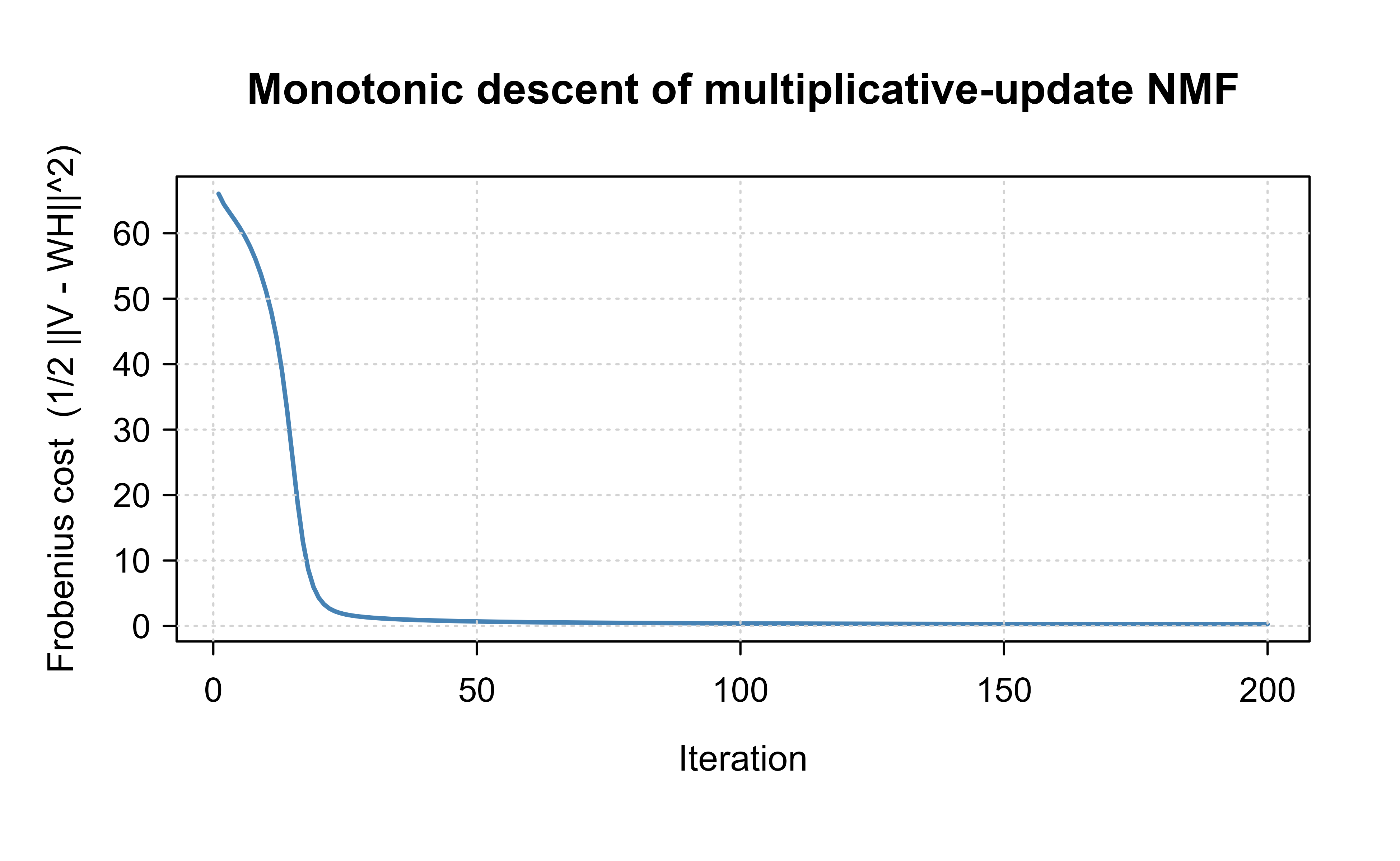
Figure 29.1: Frobenius reconstruction error of the multiplicative-update NMF at each iteration. The curve is monotonically non-increasing, as guaranteed by the Lee-Seung auxiliary-function argument, and flattens as the iterates approach a local minimum.
The printed diagnostics confirm that no iteration increases the cost (any positive jump is at the level of floating-point noise) and that the fitted \(\mathbf{W}\mathbf{H}\) reconstructs \(\mathbf{V}\) to within a small relative error. Figure 29.1 shows the cost falling steeply and then leveling off, the signature of an algorithm settling into a local minimum.
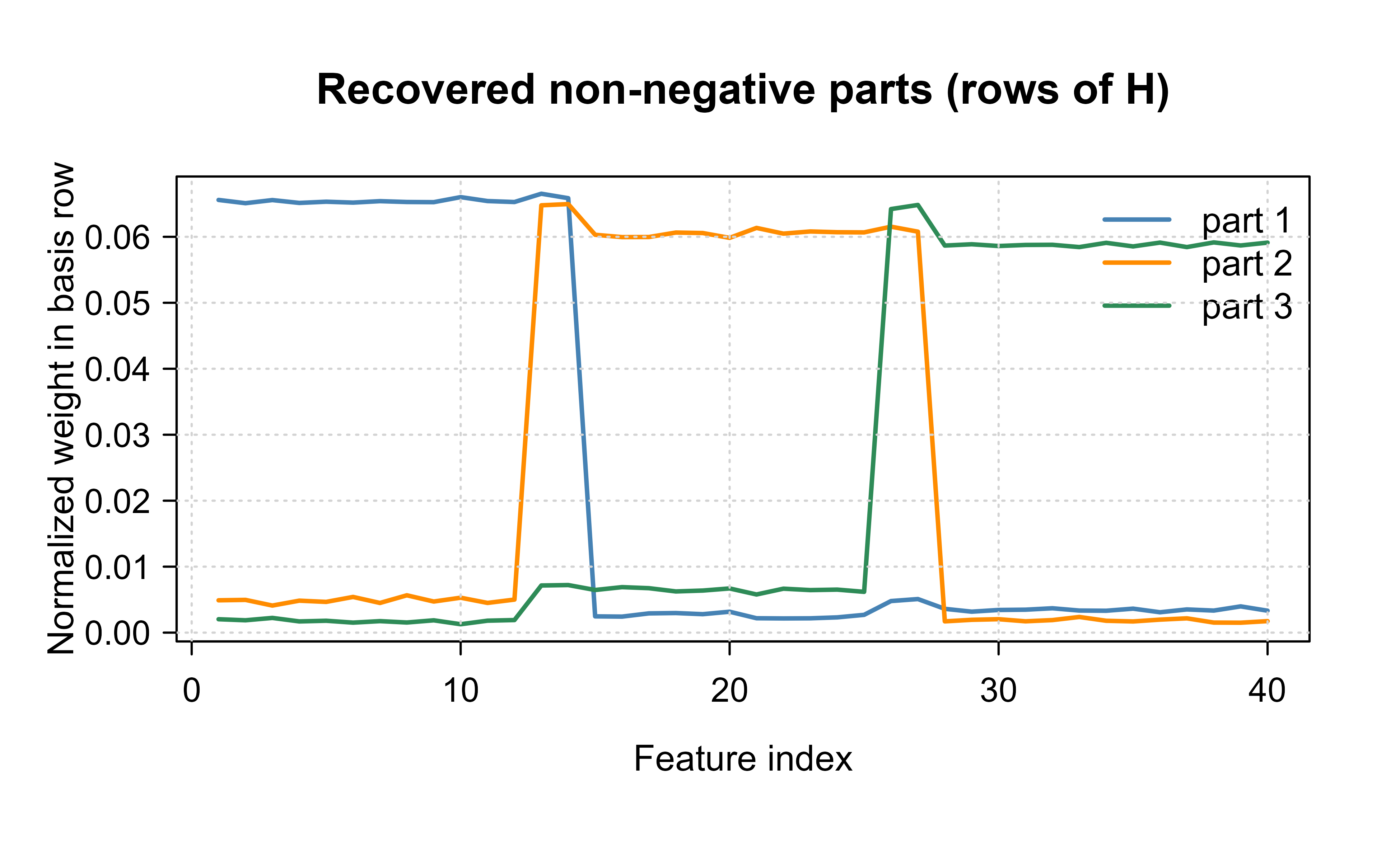
Finally, we inspect the recovered parts. Because NMF is identifiable only up to permutation and scaling, we normalize each learned basis row to unit sum before comparing it to the truth. Figure 29.2 plots the three learned rows of \(\mathbf{H}\) against the feature index; each concentrates its mass on the same contiguous block of features as one of the parts we planted, which is the parts-based behavior the non-negativity constraint is meant to produce.
Show code
H<-fit$HH_norm<-H/rowSums(H)# remove the scale ambiguity## Order learned parts by where their mass sits, for readable plottingcenter<-apply(H_norm, 1, function(h)sum(seq_len(ncol(H_norm))*h))ord<-order(center)H_norm<-H_norm[ord, , drop =FALSE]matplot(t(H_norm), type ="l", lty =1, lwd =2, col =c("steelblue", "darkorange", "seagreen"), xlab ="Feature index", ylab ="Normalized weight in basis row", main ="Recovered non-negative parts (rows of H)")legend("topright", legend =paste("part", 1:3), bty ="n", col =c("steelblue", "darkorange", "seagreen"), lwd =2)grid()
Figure 29.2: The three recovered basis rows of H (normalized to unit sum). Each learned part concentrates on a contiguous block of features, recovering the localized additive structure built into the synthetic data.
For real work you would reach for a maintained implementation. The NMF package on CRAN offers both objectives, several initializations including NNDSVD, multiple restart logic, and rank-selection diagnostics. The hand-rolled version here exists to make the update rules and their descent property concrete rather than to compete with it.
Show code
## Production NMF with the CRAN 'NMF' package (KL objective, multiple runs)library(NMF)res<-nmf(V, rank =3, method ="brunet", nrun =10, seed ="nndsvd")W<-basis(res)# n x rH<-coef(res)# r x p
29.7 Summary
NMF approximates a non-negative matrix as a product of two non-negative factors, Equation 29.1, optimizing either the Frobenius cost Equation 29.3 or the KL divergence Equation 29.4. The Lee-Seung multiplicative updates Equation 29.9 preserve non-negativity for free and are guaranteed by an auxiliary-function argument to never increase the cost. The non-negativity constraint, by forbidding cancellation, pushes the factors toward sparse additive parts, which is why NMF gives interpretable topics in text, localized features in images, and separable sources in audio. It generalizes \(k\)-means to soft additive memberships and trades PCA’s globally optimal, signed decomposition for a local, non-negative, parts-based one. The price is a non-convex objective with only local optima and factors identifiable only up to scaling and permutation, so initialization, rank selection, and multiple restarts all matter in practice.
Brunet, Jean-Philippe, Pablo Tamayo, Todd R. Golub, and Jill P. Mesirov. 2004. “Metagenes and Molecular Pattern Discovery Using Matrix Factorization.”Proceedings of the National Academy of Sciences 101 (12): 4164–69.
Lee, Daniel D., and H. Sebastian Seung. 1999. “Learning the Parts of Objects by Non-Negative Matrix Factorization.”Nature 401 (6755): 788–91.
———. 2001. “Algorithms for Non-Negative Matrix Factorization.” In Advances in Neural Information Processing Systems (NeurIPS).
Source Code
# Non-negative Matrix Factorization {#sec-nmf}```{r}#| include: falsesource("_common.R")```Many data sets are made of counts and intensities that simply cannot be negative. A document is a tally of how many times each word appears. A digitized face is a grid of pixel brightnesses. A piece of music is a spectrogram of non-negative energies across frequency and time. When we summarize such data with classical tools like principal components analysis (@sec-dimension-reduction), the building blocks we recover are free to take negative values, and a "negative amount of the word *budget*" or a "negative brightness" is hard to reason about. Non-negative matrix factorization (NMF) responds to this by insisting that every quantity in the decomposition stay non-negative, and that single constraint changes the character of the answer in a useful way: the parts it discovers tend to be interpretable pieces that add up to the whole.The guiding intuition is additive composition. If a face is built only by adding (never subtracting) a handful of localized features (an eye region here, a nose region there, a hairline), then a good summary should express each face as a non-negative blend of those features. NMF looks for exactly such a representation. It approximates a non-negative data matrix as the product of two smaller non-negative matrices: a dictionary of parts and a set of non-negative weights saying how much of each part each observation uses. Because nothing can cancel anything else out, the parts are pushed toward being sparse and localized rather than holistic. This is the sense in which NMF yields a "parts-based" representation, and it is the property that made the method famous.::: {.callout-important title="Key idea"}NMF factors a non-negative matrix $\mathbf{V}$ as $\mathbf{V} \approx \mathbf{W}\mathbf{H}$ with $\mathbf{W} \ge 0$ and $\mathbf{H} \ge 0$. The non-negativity forbids cancellation, so the recovered factors behave like additive parts rather than the signed, holistic directions of PCA.:::## The model and why parts emergeLet $\mathbf{V}$ be an $n \times p$ matrix with all entries $V_{ij} \ge 0$. Read the rows as observations (documents, faces, audio frames) and the columns as features (words, pixels, frequency bins). NMF seeks a rank-$r$ approximation$$\mathbf{V} \approx \mathbf{W}\mathbf{H}, \qquad \mathbf{W} \in \mathbb{R}_{\ge 0}^{\,n \times r}, \quad \mathbf{H} \in \mathbb{R}_{\ge 0}^{\,r \times p},$$ {#eq-nmf-model}with $r$ chosen much smaller than $\min(n,p)$. Each row of $\mathbf{H}$ is a basis vector (a "part" or, in text, a "topic") living in the original $p$-dimensional feature space, and each row of $\mathbf{W}$ holds the non-negative coordinates of one observation in that basis. Concretely, observation $i$ is reconstructed as$$V_{ij} \approx \sum_{k=1}^{r} W_{ik}\, H_{kj},$$ {#eq-nmf-entrywise}a sum of basis rows scaled by non-negative weights. Because every $W_{ik}$ and every $H_{kj}$ is non-negative, a basis vector can only ever be added in, never subtracted. To represent a face that lacks a moustache, the model cannot start from a full face and subtract one; it must instead build the face out of parts that never included a moustache in the first place. This asymmetry between addition and subtraction is what drives the factors toward sparse, localized, "part-like" structure.::: {.callout-tip title="Intuition"}Think of $\mathbf{H}$ as a box of stencils and $\mathbf{W}$ as instructions for how heavily to ink each stencil. To draw any observation you may press stencils onto the page with non-negative pressure, but you can never erase. With erasing forbidden, the only way to keep the dictionary small is for each stencil to capture a genuinely reusable piece of the data.:::It is worth being precise about what NMF does and does not promise. The constraint produces parts-based factors *empirically* on data that really is composed additively of localized parts, such as the frontal-face images in the original demonstration of @lee1999learning. It is not a theorem that every non-negative data set decomposes into clean parts. On data that is not generated additively, NMF still returns a non-negative low-rank fit, but the "parts" may be less interpretable. The interpretability is a tendency encouraged by the geometry, not a guarantee.### A geometric readingThere is a clean geometric picture. The rows of $\mathbf{W}\mathbf{H}$ are non-negative combinations of the $r$ rows of $\mathbf{H}$, so every reconstructed observation lies in the *convex cone* generated by the basis rows. NMF therefore tries to find $r$ rays (the basis vectors) whose cone wraps the data cloud as tightly as possible while staying inside the non-negative orthant. PCA, by contrast, fits an unconstrained affine subspace through the centered data; it may, and usually does, poke outside the orthant. Constraining the fit to a cone anchored at the origin is precisely what makes the factors resemble additive ingredients.## Objective functionsNMF needs a measure of how close $\mathbf{W}\mathbf{H}$ is to $\mathbf{V}$. Two cost functions dominate practice, and they correspond to two different noise models.The first is the squared Frobenius distance,$$D_{F}(\mathbf{V}\,\|\,\mathbf{W}\mathbf{H}) = \tfrac{1}{2}\,\big\| \mathbf{V} - \mathbf{W}\mathbf{H} \big\|_F^2 = \tfrac{1}{2}\sum_{i,j}\big( V_{ij} - (\mathbf{W}\mathbf{H})_{ij}\big)^2 .$$ {#eq-nmf-frob}This is the natural objective when the reconstruction error is additive and roughly Gaussian, and it is the non-negative analogue of the least-squares fit that PCA minimizes.The second is the generalized Kullback-Leibler divergence,$$D_{KL}(\mathbf{V}\,\|\,\mathbf{W}\mathbf{H}) = \sum_{i,j}\left( V_{ij}\,\log\frac{V_{ij}}{(\mathbf{W}\mathbf{H})_{ij}} - V_{ij} + (\mathbf{W}\mathbf{H})_{ij}\right).$$ {#eq-nmf-kl}Note that this is the *generalized* divergence: $\mathbf{V}$ and $\mathbf{W}\mathbf{H}$ need not sum to one, hence the extra $-V_{ij} + (\mathbf{W}\mathbf{H})_{ij}$ terms that make the divergence non-negative and zero only at a perfect fit. It is the appropriate cost when the entries are counts with Poisson noise, which is why it dominates text and count applications: maximizing the Poisson log-likelihood of $V_{ij} \sim \text{Poisson}\big((\mathbf{W}\mathbf{H})_{ij}\big)$ is the same as minimizing @eq-nmf-kl. Both objectives are bounded below by zero and equal zero exactly when $\mathbf{V} = \mathbf{W}\mathbf{H}$.::: {.callout-note title="A non-convex landscape"}In either case the objective is convex in $\mathbf{W}$ alone and convex in $\mathbf{H}$ alone, but it is *not* jointly convex in the pair $(\mathbf{W}, \mathbf{H})$. There is no closed-form global optimum and no SVD-style shortcut. Algorithms find local minima, and different initializations can give different factors. This is the price of the non-negativity constraint and the central practical difference from PCA.:::## The Lee-Seung multiplicative update rules@lee2001algorithms proposed remarkably simple iterative updates that respect non-negativity automatically and never increase the cost. We derive the Frobenius version in full, then state the KL version, then prove the monotonic-descent property.### Derivation from gradient descentFix $\mathbf{W}$ and minimize @eq-nmf-frob over $\mathbf{H} \ge 0$. The gradient with respect to a single entry $H_{kj}$ is$$\frac{\partial D_F}{\partial H_{kj}} = \big(\mathbf{W}^{\mathsf T}\mathbf{W}\mathbf{H}\big)_{kj} - \big(\mathbf{W}^{\mathsf T}\mathbf{V}\big)_{kj}.$$ {#eq-nmf-grad}A plain gradient-descent step would be $H_{kj} \leftarrow H_{kj} - \eta_{kj}\,\partial D_F/\partial H_{kj}$ for some step size $\eta_{kj}$. The trouble is that subtracting the gradient can drive an entry negative. The Lee-Seung trick is to choose a *per-entry, adaptive* step size that converts the additive update into a multiplicative one. Set$$\eta_{kj} = \frac{H_{kj}}{\big(\mathbf{W}^{\mathsf T}\mathbf{W}\mathbf{H}\big)_{kj}} .$$ {#eq-nmf-step}Substituting @eq-nmf-step and @eq-nmf-grad into the gradient step, the awkward subtraction telescopes:$$\begin{aligned}H_{kj} &\leftarrow H_{kj} - \frac{H_{kj}}{(\mathbf{W}^{\mathsf T}\mathbf{W}\mathbf{H})_{kj}}\Big[(\mathbf{W}^{\mathsf T}\mathbf{W}\mathbf{H})_{kj} - (\mathbf{W}^{\mathsf T}\mathbf{V})_{kj}\Big] \\&= H_{kj}\,\frac{(\mathbf{W}^{\mathsf T}\mathbf{V})_{kj}}{(\mathbf{W}^{\mathsf T}\mathbf{W}\mathbf{H})_{kj}} .\end{aligned}$$ {#eq-nmf-Hupdate}By the symmetric argument, holding $\mathbf{H}$ fixed and minimizing over $\mathbf{W} \ge 0$ gives$$W_{ik} \leftarrow W_{ik}\,\frac{(\mathbf{V}\mathbf{H}^{\mathsf T})_{ik}}{(\mathbf{W}\mathbf{H}\mathbf{H}^{\mathsf T})_{ik}} .$$ {#eq-nmf-Wupdate}In matrix form, with $\odot$ denoting elementwise multiplication and division applied elementwise,$$\mathbf{H} \leftarrow \mathbf{H} \odot \frac{\mathbf{W}^{\mathsf T}\mathbf{V}}{\mathbf{W}^{\mathsf T}\mathbf{W}\mathbf{H}}, \qquad\mathbf{W} \leftarrow \mathbf{W} \odot \frac{\mathbf{V}\mathbf{H}^{\mathsf T}}{\mathbf{W}\mathbf{H}\mathbf{H}^{\mathsf T}} .$$ {#eq-nmf-matrix}Three features deserve attention. First, the updates are purely multiplicative: each entry is its old value times a non-negative ratio, so non-negativity is preserved with no projection step. Second, a fixed point of @eq-nmf-Hupdate occurs exactly when the ratio equals one, that is when the gradient @eq-nmf-grad is zero (or when $H_{kj}=0$), so fixed points satisfy the Karush-Kuhn-Tucker conditions for the constrained problem. Third, an entry that ever becomes exactly zero stays zero forever, which both encourages sparsity and means a poor initialization can permanently kill a useful direction.For the KL objective @eq-nmf-kl the same auxiliary-function machinery yields$$H_{kj} \leftarrow H_{kj}\,\frac{\sum_i W_{ik}\,V_{ij}/(\mathbf{W}\mathbf{H})_{ij}}{\sum_i W_{ik}},\qquadW_{ik} \leftarrow W_{ik}\,\frac{\sum_j H_{kj}\,V_{ij}/(\mathbf{W}\mathbf{H})_{ij}}{\sum_j H_{kj}} .$$ {#eq-nmf-klupdate}### Why the cost never increasesThe descent guarantee is the heart of the Lee-Seung result. It is proved with an *auxiliary function*, the same device behind the EM algorithm. A function $G(h, h^{t})$ is an auxiliary function for $F(h)$ if$$G(h, h^{t}) \ge F(h) \quad \text{for all } h, \qquad G(h^{t}, h^{t}) = F(h^{t}).$$ {#eq-nmf-auxdef}It is an upper bound on $F$ that touches $F$ at the current iterate. If we then define the next iterate by minimizing the bound,$$h^{t+1} = \arg\min_h\, G(h, h^{t}),$$ {#eq-nmf-auxmin}we get a monotone chain,$$F(h^{t+1}) \le G(h^{t+1}, h^{t}) \le G(h^{t}, h^{t}) = F(h^{t}),$$ {#eq-nmf-monotone}where the first inequality is the upper-bound property, the second holds because $h^{t+1}$ minimizes $G$, and the equality is the touching condition. So $F$ never increases.For the Frobenius cost, treat one column of $\mathbf{H}$ at a time. Writing $F(\mathbf{h})$ for the cost as a function of that column and expanding it as the exact quadratic $F(\mathbf{h}) = F(\mathbf{h}^{t}) + (\mathbf{h}-\mathbf{h}^{t})^{\mathsf T}\nabla F(\mathbf{h}^{t}) + \tfrac{1}{2}(\mathbf{h}-\mathbf{h}^{t})^{\mathsf T}(\mathbf{W}^{\mathsf T}\mathbf{W})(\mathbf{h}-\mathbf{h}^{t})$, Lee and Seung use the auxiliary function$$G(\mathbf{h}, \mathbf{h}^{t}) = F(\mathbf{h}^{t}) + (\mathbf{h}-\mathbf{h}^{t})^{\mathsf T}\nabla F(\mathbf{h}^{t}) + \tfrac{1}{2}(\mathbf{h}-\mathbf{h}^{t})^{\mathsf T}\mathbf{K}(\mathbf{h}^{t})\,(\mathbf{h}-\mathbf{h}^{t}),$$ {#eq-nmf-auxfrob}with the diagonal matrix $K_{kk}(\mathbf{h}^{t}) = (\mathbf{W}^{\mathsf T}\mathbf{W}\mathbf{h}^{t})_{k}/h^{t}_{k}$. The key lemma is that $\mathbf{K}(\mathbf{h}^{t}) - \mathbf{W}^{\mathsf T}\mathbf{W}$ is positive semidefinite, which makes $G$ an upper bound that touches $F$ at $\mathbf{h}^{t}$. Because $\mathbf{K}$ is diagonal, the minimizer of @eq-nmf-auxfrob has the closed form $\mathbf{h}^{t+1} = \mathbf{h}^{t} - \mathbf{K}^{-1}\nabla F(\mathbf{h}^{t})$, and substituting $\mathbf{K}$ reproduces exactly the multiplicative update @eq-nmf-Hupdate. The same construction with a log-based auxiliary function (using Jensen's inequality on the concave logarithm) handles the KL cost and yields @eq-nmf-klupdate. The practical payoff is a guarantee worth stating plainly.::: {.callout-important title="Monotonic descent"}Under the multiplicative updates @eq-nmf-matrix (Frobenius) or @eq-nmf-klupdate (KL), the cost is non-increasing at every step. Because the cost is bounded below by zero, the sequence of objective values converges. This is convergence of the *objective*, not a guarantee of reaching the global minimum; the iterates may settle at any local stationary point.:::## Practical matters### Choosing the rankThe rank $r$ is the one essential hyperparameter, analogous to the number of components in PCA (@sec-dimension-reduction) or the number of clusters in $k$-means (@sec-cluster). Common strategies:- Plot the residual fit error (reconstruction RMSE or KL divergence) against $r$ and look for the elbow where adding factors stops paying off.- Use a held-out mask: hide a random subset of entries, fit on the rest, and choose the $r$ that best predicts the held-out entries. This guards against simply memorizing noise.- For exploratory work, judge interpretability directly. The "right" number of topics or parts is often the one whose factors a domain expert can name.- More formal criteria include the cophenetic correlation of @brunet2004metagenes, which measures how stably samples cluster across many random restarts as $r$ varies.Because the objective is non-convex, the result depends on initialization. Random non-negative starts are simplest, but running several restarts and keeping the best fit is standard. A popular deterministic alternative is non-negative double SVD (NNDSVD), which seeds $\mathbf{W}$ and $\mathbf{H}$ from the leading singular vectors of $\mathbf{V}$ with negative parts removed, giving faster and more reproducible convergence.### Scaling, complexity, and failure modesEach multiplicative iteration costs a few dense matrix products, dominated by the $\mathcal{O}(n p r)$ work to form $\mathbf{W}\mathbf{H}$ and the cross-products, so a sweep is linear in the number of data entries for fixed $r$. This scales well to large sparse count matrices, where the products exploit sparsity.A few hazards recur in practice:- The factorization is not unique. For any invertible non-negative matrix $\mathbf{B}$ with non-negative inverse (for instance a permutation or positive diagonal scaling), $\mathbf{W}\mathbf{H} = (\mathbf{W}\mathbf{B})(\mathbf{B}^{-1}\mathbf{H})$ is an equally good fit. Factors are therefore identifiable only up to scaling and permutation, and one usually normalizes the rows of $\mathbf{H}$ to remove the scale ambiguity.- Division by zero in the updates is avoided by adding a tiny $\varepsilon$ to denominators.- Zeros are absorbing. An entry driven to exactly zero never revives, so an unlucky start can collapse a factor.- Convergence of the objective does not imply the iterates have converged; monitor the relative change in $\mathbf{W}$ and $\mathbf{H}$, not just the cost.::: {.callout-warning}NMF has no built-in centering or scaling, and it must not be mean-centered, because centering would introduce negative values and destroy the very constraint the method relies on. Standardizing columns to comparable magnitudes (for example TF-IDF weighting of a document-term matrix) is fine and often helps, as long as the result stays non-negative.:::## Relation to k-means and PCANMF sits between two methods you already know, and seeing the connections clarifies what it buys you.Compared with **PCA** (@sec-dimension-reduction), both seek a rank-$r$ approximation $\mathbf{V} \approx \mathbf{W}\mathbf{H}$ that minimizes squared error. PCA leaves $\mathbf{W}$ and $\mathbf{H}$ unconstrained except for orthogonality and solves the problem globally and uniquely through the SVD. NMF drops orthogonality, adds $\mathbf{W},\mathbf{H} \ge 0$, and consequently loses both the closed form and the uniqueness. The reward is interpretability: PCA components are signed and holistic (each one redistributes brightness across the whole image), whereas NMF parts are non-negative and tend to be localized. PCA reconstructs by cancellation, NMF by addition. PCA also captures the most variance for a given rank, so it usually achieves a smaller reconstruction error than NMF at the same $r$; you trade a little fit for a lot of interpretability.Compared with **$k$-means** (@sec-cluster), NMF is a soft, additive generalization. Hard $k$-means can be written as a matrix factorization $\mathbf{V} \approx \mathbf{W}\mathbf{H}$ in which $\mathbf{H}$ holds the cluster centroids and each row of $\mathbf{W}$ is a one-hot indicator selecting a single centroid. If we constrain each row of $\mathbf{W}$ in NMF to have exactly one nonzero entry, we recover $k$-means. NMF relaxes that to allow each observation to be a non-negative blend of several "centroids," so an observation can belong partly to topic 1 and partly to topic 3. In this light NMF is to $k$-means roughly what a soft mixture is to a hard assignment.These ties also connect NMF to nearby ideas in this book: it is the linear, count-friendly cousin of the topic models and the non-negative bottleneck layers that appear in autoencoders (@sec-autoencoders), and the Poisson/KL formulation links it to the multinomial likelihoods used in naive Bayes text models (@sec-naive-bayes). Its use in collaborative filtering, factoring a sparse non-negative user-by-item matrix, is the workhorse behind much of @sec-recommender-systems.## A runnable demonstrationWe implement the Frobenius multiplicative updates from scratch in base R on a small non-negative matrix and verify the two facts the theory promises: the objective decreases monotonically, and the recovered factors approximately reconstruct the data. To make the parts-based behavior visible, we build $\mathbf{V}$ from three known non-negative "parts" plus a little noise, so we know there is genuine additive structure to find.```{r}#| label: fig-nmf-convergence#| fig-cap: "Frobenius reconstruction error of the multiplicative-update NMF at each iteration. The curve is monotonically non-increasing, as guaranteed by the Lee-Seung auxiliary-function argument, and flattens as the iterates approach a local minimum."set.seed(1301)## --- Build a non-negative matrix with known additive parts ---------------n <-60# observationsp <-40# featuresr <-3# true number of parts## Three localized, non-negative "parts" (rows of H_true)H_true <-matrix(0, nrow = r, ncol = p)H_true[1, 1:14] <-1# part 1 lives in features 1-14H_true[2, 13:27] <-1# part 2 overlaps part 1 a littleH_true[3, 26:40] <-1# part 3 lives in features 26-40## Each observation uses a non-negative blend of the partsW_true <-matrix(runif(n * r, 0, 1), nrow = n, ncol = r)V <- W_true %*% H_trueV <- V +matrix(runif(n * p, 0, 0.05), nrow = n, ncol = p) # non-negative noiseV[V <0] <-0# stay non-negative## --- Frobenius objective -------------------------------------------------frob_cost <-function(V, W, H) 0.5*sum((V - W %*% H)^2)## --- NMF via Lee-Seung multiplicative updates ----------------------------nmf_mult <-function(V, r, n_iter =200, eps =1e-9, seed =1) {set.seed(seed) n <-nrow(V); p <-ncol(V) W <-matrix(runif(n * r, 0.1, 1), n, r) # strictly positive start H <-matrix(runif(r * p, 0.1, 1), r, p) cost <-numeric(n_iter)for (t inseq_len(n_iter)) {## Update H: H <- H * (W^T V) / (W^T W H) H <- H * (crossprod(W, V) / (crossprod(W, W) %*% H + eps))## Update W: W <- W * (V H^T) / (W H H^T) W <- W * (tcrossprod(V, H) / (W %*%tcrossprod(H, H) + eps)) cost[t] <-frob_cost(V, W, H) }list(W = W, H = H, cost = cost)}fit <-nmf_mult(V, r = r, n_iter =200, seed =42)## --- Verify monotonic descent --------------------------------------------diffs <-diff(fit$cost)cat("Max iteration-to-iteration increase in cost:",formatC(max(diffs), format ="e", digits =3), "\n")cat("Monotonically non-increasing (within tolerance):",all(diffs <=1e-6), "\n")cat("Initial cost:", round(fit$cost[1], 3)," Final cost:", round(tail(fit$cost, 1), 3), "\n")## --- Reconstruction quality ----------------------------------------------V_hat <- fit$W %*% fit$Hrel_err <-sqrt(sum((V - V_hat)^2)) /sqrt(sum(V^2))cat("Relative reconstruction error:", round(rel_err, 4), "\n")## --- Plot the convergence curve ------------------------------------------plot(seq_along(fit$cost), fit$cost, type ="l", lwd =2, col ="steelblue",xlab ="Iteration", ylab ="Frobenius cost (1/2 ||V - WH||^2)",main ="Monotonic descent of multiplicative-update NMF")grid()```The printed diagnostics confirm that no iteration increases the cost (any positive jump is at the level of floating-point noise) and that the fitted $\mathbf{W}\mathbf{H}$ reconstructs $\mathbf{V}$ to within a small relative error. @fig-nmf-convergence shows the cost falling steeply and then leveling off, the signature of an algorithm settling into a local minimum.Finally, we inspect the recovered parts. Because NMF is identifiable only up to permutation and scaling, we normalize each learned basis row to unit sum before comparing it to the truth. @fig-nmf-parts plots the three learned rows of $\mathbf{H}$ against the feature index; each concentrates its mass on the same contiguous block of features as one of the parts we planted, which is the parts-based behavior the non-negativity constraint is meant to produce.```{r}#| label: fig-nmf-parts#| fig-cap: "The three recovered basis rows of H (normalized to unit sum). Each learned part concentrates on a contiguous block of features, recovering the localized additive structure built into the synthetic data."H <- fit$HH_norm <- H /rowSums(H) # remove the scale ambiguity## Order learned parts by where their mass sits, for readable plottingcenter <-apply(H_norm, 1, function(h) sum(seq_len(ncol(H_norm)) * h))ord <-order(center)H_norm <- H_norm[ord, , drop =FALSE]matplot(t(H_norm), type ="l", lty =1, lwd =2,col =c("steelblue", "darkorange", "seagreen"),xlab ="Feature index", ylab ="Normalized weight in basis row",main ="Recovered non-negative parts (rows of H)")legend("topright", legend =paste("part", 1:3), bty ="n",col =c("steelblue", "darkorange", "seagreen"), lwd =2)grid()```For real work you would reach for a maintained implementation. The `NMF` package on CRAN offers both objectives, several initializations including NNDSVD, multiple restart logic, and rank-selection diagnostics. The hand-rolled version here exists to make the update rules and their descent property concrete rather than to compete with it.```{r}#| eval: false## Production NMF with the CRAN 'NMF' package (KL objective, multiple runs)library(NMF)res <-nmf(V, rank =3, method ="brunet", nrun =10, seed ="nndsvd")W <-basis(res) # n x rH <-coef(res) # r x p```## SummaryNMF approximates a non-negative matrix as a product of two non-negative factors, @eq-nmf-model, optimizing either the Frobenius cost @eq-nmf-frob or the KL divergence @eq-nmf-kl. The Lee-Seung multiplicative updates @eq-nmf-matrix preserve non-negativity for free and are guaranteed by an auxiliary-function argument to never increase the cost. The non-negativity constraint, by forbidding cancellation, pushes the factors toward sparse additive parts, which is why NMF gives interpretable topics in text, localized features in images, and separable sources in audio. It generalizes $k$-means to soft additive memberships and trades PCA's globally optimal, signed decomposition for a local, non-negative, parts-based one. The price is a non-convex objective with only local optima and factors identifiable only up to scaling and permutation, so initialization, rank selection, and multiple restarts all matter in practice.