Almost every model in this book so far has come with its own machinery for finding the best parameters. Ordinary least squares has a formula. glmnet has a coordinate descent routine written in Fortran. xgboost has its own boosting engine. You call one function, and the fitting happens out of sight. torch takes the opposite stance: it hands you the raw ingredients (numbers in tensors, a way to compute derivatives automatically, and a set of optimizers) and lets you assemble the model and write the training loop yourself. That sounds like more work, and it is, but it is also the only way to fit a model that no package ships, and it is the foundation on which deep learning and modern AI systems are built.
The torch package brings the LibTorch C++ library (the engine behind PyTorch) to R without any Python dependency.1 It gives R users tensors, automatic differentiation, neural network building blocks, optimizers, and data loading, all as native R objects. If you have written models in PyTorch, the API will feel familiar. If you have only used keras/tensorflow from R, torch offers a lower level, more imperative style where you write the training loop yourself.
By the end of this chapter you should understand three things: where torch sits among the fitting engines you already know, why gradient descent and automatic differentiation (the math underneath every torch program) actually work, and how a torch script is structured in practice (tensors, autograd, nn_module, optimizers, datasets, and dataloaders). Because torch is often not installed on a given machine, all torch code here is shown with eval=FALSE; it is correct and idiomatic, just not executed during the build. To teach the core mechanics in a way you can run immediately, the chapter ends with a worked example that implements gradient descent for linear regression in plain base R with hand derived gradients. That demo mirrors the torch training loop line for line, so once you see it work you will know exactly what the torch version is doing under the hood.
Key idea
torch is not a model. It is a toolkit for building and training any model you can write as a differentiable function of its parameters. The loss, the architecture, and the update rule are all yours to specify.
Most of the supervised methods in earlier chapters either have closed form estimators (ordinary least squares), or rely on a specialized optimizer baked into a package (glmnet for penalized regression, xgboost for boosted trees). torch is different in kind: it is a general purpose engine for fitting any model you can write as a differentiable function of parameters, by following gradients downhill.
The way to think about it is that a torch program has three layers, and you, not the package, decide what goes in each. The first layer is a model, expressed as a function \(f(\mathbf{x}; \boldsymbol{\theta})\) that turns inputs into predictions using parameters \(\boldsymbol{\theta}\). The second layer is a loss \(L(\boldsymbol{\theta})\), a single number that measures how badly the predictions match the targets. The third layer is an optimizer, which nudges \(\boldsymbol{\theta}\) in the direction that reduces the loss, using the gradient \(\nabla_{\boldsymbol{\theta}} L\).3 The remarkable thing is that torch computes that gradient for you, automatically, no matter how complicated the model, through a mechanism called automatic differentiation (autograd).
This same three layer recipe describes linear regression, logistic regression, deep neural networks, and large language models alike; only the model and the loss change. That generality is the whole point. Once you understand the loop, you can fit custom losses (quantile, as in quantile regression (Chapter 21), Huber, ranking), custom architectures (embeddings, attention as in the transformers chapter (Chapter 38), convolutions), and models that simply do not exist as off the shelf packages, all in R, on CPU or GPU.
When to use this
Reach for torch when you need a model that no R package provides, or a custom loss or constraint; when you want GPU acceleration for large tensor computations; or when you are prototyping deep learning in a pure R stack and want fine control of the training loop.
The flip side matters just as much, because torch is easy to overuse. If a linear model, a GAM, or gradient boosted trees already solves your problem, prefer them: they are faster to fit, easier to tune, and on tabular data they are often more accurate than a neural network you would have to babysit. And if your goal is maximum performance on very large models with a mature surrounding ecosystem, that work still mostly lives in Python. torch is the right tool for custom modeling and learning in R, not a reason to abandon the simpler methods that win on structured data.
92.2 The math: gradient descent and autograd
Before writing any torch code, it helps to see what the optimizer is actually doing. The whole of gradient based training rests on one simple picture: the loss is a landscape over the parameter space, and we want to walk downhill to the lowest valley. This section makes that picture precise, works out the gradient for linear regression by hand, and then explains what autograd does so that you never have to work out a gradient by hand again.
92.2.1 The optimization problem
Let the training data be pairs \((\mathbf{x}_i, y_i)\) for \(i = 1, \dots, n\), with \(\mathbf{x}_i \in \mathbb{R}^p\). A model produces predictions \(\hat y_i = f(\mathbf{x}_i; \boldsymbol{\theta})\), and we choose \(\boldsymbol{\theta}\) to minimize an average loss
where \(\eta > 0\) is the learning rate, the size of the step we take each iteration. Stochastic gradient descent (SGD) replaces the full sum with the gradient computed on a small randomly chosen batch of examples, which is cheaper per step and, perhaps surprisingly, the noise it injects often helps the optimizer escape poor regions of the landscape.
Intuition
Picture the loss as a hilly surface and \(\boldsymbol{\theta}\) as your position on it. The gradient points uphill, so the update rule above takes a step in the opposite direction, downhill. The learning rate \(\eta\) sets how far each step goes: too small and you inch along forever, too large and you overshoot the valley and bounce around (or fly off to infinity).
92.2.2 Linear regression gradient
Take the squared error loss with a linear model \(f(\mathbf{x}_i; \boldsymbol{\theta}) = \mathbf{x}_i^\top \boldsymbol{\beta} + b\), so \(\boldsymbol{\theta} = (\boldsymbol{\beta}, b)\). Writing \(r_i = y_i - (\mathbf{x}_i^\top \boldsymbol{\beta} + b)\) for the residual,
\[
L(\boldsymbol{\beta}, b) = \frac{1}{n} \sum_{i=1}^{n} r_i^2 .
\]
In matrix form, with design matrix \(\mathbf{X}\) (rows \(\mathbf{x}_i^\top\)), residual vector \(\mathbf{r} = \mathbf{y} - (\mathbf{X}\boldsymbol{\beta} + b\mathbf{1})\),
\[
\nabla_{\boldsymbol{\beta}} L = -\frac{2}{n} \mathbf{X}^\top \mathbf{r},
\qquad
\nabla_{b} L = -\frac{2}{n} \mathbf{1}^\top \mathbf{r}.
\]
For this loss the minimum has a closed form (\(\hat{\boldsymbol{\beta}} = (\mathbf{X}^\top \mathbf{X})^{-1}\mathbf{X}^\top \mathbf{y}\) after centering), which we use below as a check. Gradient descent reaches the same answer iteratively, and unlike the closed form it generalizes to losses and models with no analytic solution. That is the lesson to carry forward: we use linear regression here only because we can verify the answer, not because gradient descent is the smart way to fit it.
92.2.3 What autograd actually does
Notice how much algebra it took to write down that gradient, and that was for the simplest possible model. For a network with several layers, deriving the gradient by hand is error prone and, once the model changes, has to be redone. Autograd removes that step entirely.
The mechanism is easier than it sounds. As you compute the loss, torch watches every operation you apply to tensors marked requires_grad = TRUE and records them as a graph, where each node is one operation and remembers how to differentiate its output with respect to its inputs (its local Jacobian).4 When you call loss$backward(), torch walks that graph backward from the loss to the parameters, multiplying the local derivatives together by the chain rule. This is reverse mode automatic differentiation, and it is identical to the backpropagation algorithm you may have heard described for neural networks (Chapter 15).
There are really only two phases to keep straight. In the forward pass you compute the loss as usual, and torch quietly records the operations. In the backward pass, the single call loss$backward() fills each parameter’s $grad field with \(\partial L / \partial \theta\), ready for the optimizer to use.
Key idea
Reverse mode autograd computes the derivative of one scalar output (the loss) with respect to all of the parameters in a single backward pass, at roughly the cost of one forward pass. That efficiency, independent of how many parameters there are, is precisely why training models with millions of parameters is feasible at all.
92.3 A torch program, end to end
With the math in hand, we can look at how a real torch program is organized. The pieces below appear in nearly every script: tensors hold the data, autograd produces the gradients, an nn_module packages the model, an optimizer applies the updates, and a dataset plus dataloader feed in batches. Read them in order, because each builds on the last, and watch for the four line training loop, which is the part you will type most often.
The code below shows the canonical torch structure. It is eval=FALSE because torch may not be installed on the build machine, but it is current, runnable code.
92.3.1 Tensors
A tensor is torch’s version of an array: a multidimensional grid of numbers that can live on a CPU or a GPU and that knows how to track gradients. A scalar is a 0D tensor, a vector is 1D, a matrix is 2D, and an image batch might be 4D. Everything else in torch operates on tensors.
Show code
library(torch)# create tensorsx<-torch_tensor(matrix(rnorm(6), nrow =3))# 3 x 2 float tensory<-torch_tensor(c(1, 2, 3))x$shape# dimensionsx$dtype# data typex+1# elementwisetorch_mm(x, x$t())# matrix multiply (3x2 %*% 2x3 = 3x3)# move to GPU if availableif(cuda_is_available()){x<-x$to(device ="cuda")}
92.3.2 Autograd by hand
To see autograd in isolation, it helps to use a function simple enough to differentiate in your head. The snippet below computes a gradient with autograd and confirms it against the value you would get by hand, which is the same idea the runnable demo at the end of the chapter will show without torch at all.
Show code
library(torch)w<-torch_tensor(2.0, requires_grad =TRUE)# f(w) = w^2 + 3w -> df/dw = 2w + 3 = 7 at w = 2fval<-w^2+3*wfval$backward()w$grad# tensor of 7
92.3.3 Defining a model with nn_module
An nn_module is the standard container for a model: it bundles the parameters together with a forward method that says how to turn an input into a prediction. The pattern is always the same, you create the layers in initialize and chain them in forward. A linear regression is just one nn_linear layer; a deep network stacks several with nonlinear activations in between.5
Show code
library(torch)linreg<-nn_module("linreg", initialize =function(in_features){self$fc<-nn_linear(in_features, 1)}, forward =function(x){self$fc(x)})# a small multilayer perceptron for comparisonmlp<-nn_module("mlp", initialize =function(in_features, hidden){self$fc1<-nn_linear(in_features, hidden)self$fc2<-nn_linear(hidden, 1)}, forward =function(x){x%>%self$fc1()%>%nnf_relu()%>%self$fc2()})
92.3.4 The training loop
This is the heart of torch, and it is worth reading slowly, because every model you ever train will use some version of it. Compare each line to the base R demo at the end of the chapter, where the same steps appear without any torch machinery.
Show code
library(torch)set.seed(1)n<-500; p<-3X<-matrix(rnorm(n*p), n, p)beta_true<-c(1.5, -2.0, 0.5)y<-as.numeric(X%*%beta_true+0.7)+rnorm(n, sd =0.3)x_t<-torch_tensor(X, dtype =torch_float())y_t<-torch_tensor(matrix(y, ncol =1), dtype =torch_float())model<-linreg(in_features =p)optimizer<-optim_adam(model$parameters, lr =0.05)loss_fn<-nnf_mse_lossn_epochs<-200for(epochinseq_len(n_epochs)){optimizer$zero_grad()# clear old gradientspred<-model(x_t)# forward passloss<-loss_fn(pred, y_t)# compute lossloss$backward()# autograd: fills $gradoptimizer$step()# update parametersif(epoch%%50==0){cat(sprintf("epoch %d loss %.4f\n", epoch, loss$item()))}}# recover learned coefficients and interceptmodel$parameters$fc.weightmodel$parameters$fc.bias
The four steps inside that loop, clear the old gradients, run the forward pass to get the loss, call backward to fill in the gradients, then step to update the parameters, are the universal torch rhythm. Memorize them in that order and you can train almost anything.
Warning
optimizer$zero_grad() is not optional. torch adds new gradients to whatever is already in $grad rather than replacing them, a design that is useful for some advanced techniques but means that if you forget to clear, your gradients accumulate across steps and training quietly goes wrong. This is the single most common beginner bug.
92.3.5 Datasets and dataloaders
The loop above fed the entire dataset to the model at once. That is fine for a few hundred rows, but when data is large, will not fit in memory, or should be shuffled into random minibatches, you wrap it in a dataset (which defines how to fetch one example) and iterate with a dataloader (which handles batching and shuffling for you).
It helps to place torch next to the other fitting engines you have already met, so you can see what you trade by choosing it. Table 92.1 positions torch against them along the dimensions that matter in practice: what runs underneath, whether the API is imperative or declarative, what each tool is best at, and whether you write the training loop yourself.
Table 92.1: Comparison of torch with the other model fitting engines used in this book, across backend, API style, typical use case, GPU support, and whether the user writes the training loop.
Tool
Engine / backend
API style
Best for
GPU
Writes own training loop
torch
LibTorch (C++)
imperative, define by run
custom models, custom losses, research style deep learning
Yes
Yes
keras/tensorflow
TensorFlow (C++)
declarative fit(), layers
standard deep nets, quick prototypes
Yes
No (usually)
glmnet
Fortran coordinate descent
one glmnet() call
penalized linear/logistic regression
No
No
xgboost / lightgbm
C++ gradient boosting
one fit call
tabular prediction, strong default accuracy
Yes (xgboost)
No
base R lm/optim
LAPACK / general optimizers
function call
closed form or general purpose optimization
No
Sometimes
Within a torch loop you also choose an optimizer, the rule that turns gradients into parameter updates. The variants differ mainly in how much they adapt the step size and how much tuning they demand. Table 92.2 sketches the common choices; if you are unsure, start with Adam.
Table 92.2: Common torch optimizers, their update rules in brief, the tuning effort each demands, and practical notes on when to use them.
Optimizer
Update rule (sketch)
Tuning burden
Notes
SGD
\(\theta \leftarrow \theta - \eta \nabla L\)
learning rate, maybe momentum
simple, robust with a good schedule
SGD + momentum
velocity \(v \leftarrow \mu v - \eta \nabla L\), then \(\theta \leftarrow \theta + v\)
\(\eta\), \(\mu\)
smooths noisy gradients
RMSprop
scale step by running mean of squared gradients
\(\eta\)
good for nonstationary objectives
Adam
combines momentum and RMSprop with bias correction
\(\eta\) (forgiving)
strong default, optim_adam
92.5 Runnable demo: gradient descent in base R
Everything so far has been eval=FALSE, so to make the ideas concrete here is a version you can run today. This demo reproduces the torch training loop with no torch, no autograd, and the manual gradients we derived earlier. Because it uses only base R, it executes during the build, and because it solves the same linear regression problem two ways (gradient descent and the closed form), you can check that the loop really converges to the right answer.
Tip
As you read the demo, keep the torch loop in mind. The base R pred plays the role of model(x), the mean of r^2 is nnf_mse_loss, the two grad_* lines are what loss$backward() would compute for you, and the subtraction step is optimizer$step(). Seeing them side by side is the fastest way to demystify torch.
We begin by simulating data from a known linear model and computing the closed form least squares fit, which serves as the target the iterative method should reach.
Show code
set.seed(42)# simulate linear regression datan<-400p<-2X<-matrix(rnorm(n*p), n, p)beta_true<-c(2.0, -1.0)b_true<-0.5y<-as.numeric(X%*%beta_true+b_true)+rnorm(n, sd =0.4)# closed form least squares for reference (with intercept column)Xd<-cbind(1, X)theta_ols<-solve(crossprod(Xd), crossprod(Xd, y))b_ols<-theta_ols[1]beta_ols<-theta_ols[-1]round(c(b =b_ols, beta1 =beta_ols[1], beta2 =beta_ols[2]), 4)#> b beta1 beta2 #> 0.5049 1.9960 -1.0078
Now the gradient descent loop. Each iteration mirrors one torch epoch: forward pass (predictions), loss, backward pass (analytic gradient), and the parameter update.
Show code
# initialize parameters at zero, like a fresh nn_linearbeta<-rep(0, p)b<-0eta<-0.1# learning raten_epochs<-200loss_history<-numeric(n_epochs)for(epochinseq_len(n_epochs)){# forward passpred<-as.numeric(X%*%beta+b)r<-y-pred# residuals# loss (mean squared error)loss_history[epoch]<-mean(r^2)# backward pass: analytic gradients of MSEgrad_beta<--(2/n)*as.numeric(t(X)%*%r)grad_b<--(2/n)*sum(r)# parameter update (the "optimizer step")beta<-beta-eta*grad_betab<-b-eta*grad_b}round(c(b =b, beta1 =beta[1], beta2 =beta[2]), 4)#> b beta1 beta2 #> 0.5049 1.9960 -1.0078
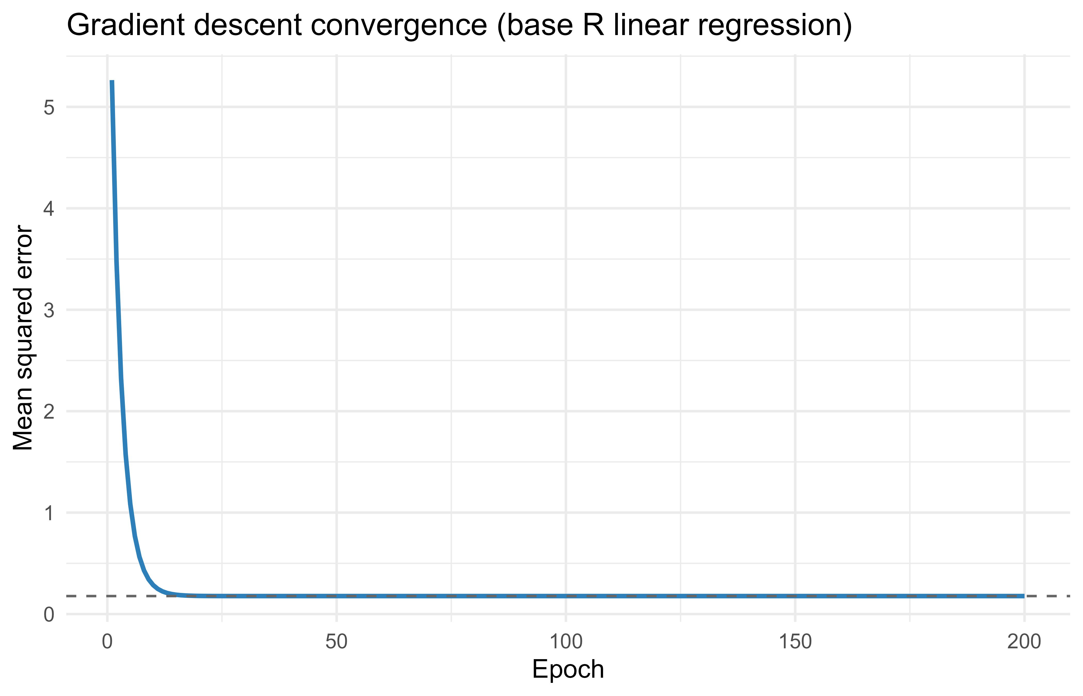
If the loop worked, these gradient descent estimates should sit right on top of the closed form least squares solution printed above. They do, which tells us the hand derived gradients and the update rule are correct. To see the convergence rather than just the endpoint, Figure 92.1 plots the loss at every epoch.
Show code
library(ggplot2)# loss at the OLS optimum, for referenceols_loss<-mean((y-as.numeric(X%*%beta_ols+b_ols))^2)loss_df<-data.frame(epoch =seq_len(n_epochs), loss =loss_history)ggplot(loss_df, aes(epoch, loss))+geom_line(color ="#2c7fb8", linewidth =1)+geom_hline(yintercept =ols_loss, linetype ="dashed", color ="grey40")+labs( title ="Gradient descent convergence (base R linear regression)", x ="Epoch", y ="Mean squared error")+theme_minimal(base_size =12)
Figure 92.1: Mean squared error loss across gradient descent epochs for the base R linear regression demo. The dashed line marks the loss at the closed form least squares solution.
The loss falls steeply at first and then flattens as it settles onto the dashed line marking the least squares optimum, the textbook shape of a well behaved gradient descent run. Finally, Table 92.3 lays the two solutions side by side so the agreement is unmistakable.
Show code
compare<-data.frame( parameter =c("intercept", "beta1", "beta2"), closed_form =round(c(b_ols, beta_ols), 4), grad_descent =round(c(b, beta), 4))knitr::kable(compare, caption ="Closed form least squares estimates compared with the gradient descent estimates for the base R linear regression demo, parameter by parameter.", col.names =c("Parameter", "Closed form", "Gradient descent"))
Table 92.3: Closed form least squares estimates compared with the gradient descent estimates for the base R linear regression demo, parameter by parameter.
Parameter
Closed form
Gradient descent
intercept
0.5049
0.5049
beta1
1.9960
1.9960
beta2
-1.0078
-1.0078
The mapping back to torch is exact: our pred is model(x), our mean of r^2 is nnf_mse_loss, our grad_beta and grad_b are what loss$backward() computes automatically, and our subtraction step is optimizer$step(). The only thing torch adds is that you no longer derive the gradients yourself. That single convenience is what turns the loop you just ran on a two parameter model into a method that trains networks with millions of parameters.
92.6 Practical guidance and pitfalls
The examples above run cleanly because they are small and well scaled. Real torch work runs into a recurring set of snags, and knowing them in advance saves hours of debugging. The most common failure is forgetting to clear gradients: always call optimizer$zero_grad() before backward(), since torch accumulates gradients and skipping this sums them across steps. Shape and type mismatches are the next most common: targets for nnf_mse_loss should usually be a column tensor (ncol = 1) so they line up with the model output, because broadcasting against a 1D target silently changes the loss into something you did not intend.
Convergence problems almost always trace back to two causes, and both are easy to fix. Unscaled inputs are the first: gradient descent is sensitive to feature scale, so center and scale your columns before training, exactly the advice you saw for glmnet. The learning rate is the second, and it is the first knob to tune. Too large and the loss diverges to NaN; too small and it crawls. A sensible starting point is optim_adam(lr = 0.01), adjusted up or down by factors of about three. If the loss turns into NaN, suspect a learning rate that is too high, unscaled inputs, or a logarithm of a non positive number inside a custom loss.
Warning
torch keeps its own random number stream. Setting R’s set.seed() does not make torch reproducible. Use torch_manual_seed() as well to fix the initialization and the shuffling order.
A few habits round out good practice. At prediction time, put the model in evaluation mode with model$eval() and wrap the call in with_no_grad(), so layers like dropout and batch normalization behave correctly and you do not build a backward graph you will never use. Before committing to a neural network on tabular data, benchmark against gradient boosted trees (Chapter 12) or a generalized additive model (Chapter 6), which frequently win on structured data with far less tuning. And remember that GPU acceleration pays off only when tensors are large; for small tabular problems the cost of moving data to the GPU outweighs the speedup, and the CPU is faster.
When to use this
In short, default to the simpler model, reach for torch when the problem genuinely needs a custom architecture or loss, scale your inputs, tune the learning rate first, and seed torch separately. Follow those and most training problems disappear.
92.7 Further reading
Goodfellow, Bengio, and Courville (2016), Deep Learning, for backpropagation and optimization theory.
Chollet and Allaire (2022), Deep Learning with R, 2nd edition, for applied deep learning in R.
Kingma and Ba (2015), Adam: A Method for Stochastic Optimization, for the Adam optimizer.
Paszke et al. (2019), PyTorch: An Imperative Style, High Performance Deep Learning Library, for the design of the underlying engine.
Baydin, Pearlmutter, Radul, and Siskind (2018), Automatic Differentiation in Machine Learning: a Survey, for reverse mode autograd.
The torch for R documentation at torch.mlverse.org for current API reference and examples.
Chollet, Francois, Tomasz Kalinowski, and J. J. Allaire. 2022. Deep Learning with r. 2nd ed. Manning Publications.
Goodfellow, Ian, Yoshua Bengio, and Aaron Courville. 2016. Deep Learning. MIT Press.
This is worth emphasizing because the older R route to deep learning, keras/tensorflow, calls into a Python installation behind the scenes, which can be fragile to set up. torch installs as a normal R package and links to a precompiled C++ library, so there is no Python to manage.↩︎
The gradient is the vector of partial derivatives of the loss with respect to every parameter. It points in the direction of steepest increase, so stepping the opposite way decreases the loss. Computing it is the one genuinely hard part, and it is exactly the part torch automates.↩︎
A Jacobian is just the matrix of partial derivatives of a vector valued function. For a single operation like addition or matrix multiply it is small and known in closed form, which is why torch can store the rule for it.↩︎
The activation, here nnf_relu (rectified linear unit, which returns max(0, x)), is what lets a stack of linear layers represent nonlinear functions. Without a nonlinearity between them, two linear layers collapse into a single linear layer.↩︎
Source Code
# torch for R {#sec-torch-for-r}```{r}#| include: falsesource("_common.R")```Almost every model in this book so far has come with its own machinery for finding the best parameters. Ordinary least squares has a formula. `glmnet` has a coordinate descent routine written in Fortran. `xgboost` has its own boosting engine. You call one function, and the fitting happens out of sight. `torch` takes the opposite stance: it hands you the raw ingredients (numbers in tensors, a way to compute derivatives automatically, and a set of optimizers) and lets you assemble the model and write the training loop yourself. That sounds like more work, and it is, but it is also the only way to fit a model that no package ships, and it is the foundation on which deep learning and modern AI systems are built.The `torch` package brings the LibTorch C++ library (the engine behind PyTorch) to R without any Python dependency.^[This is worth emphasizing because the older R route to deep learning, `keras`/`tensorflow`, calls into a Python installation behind the scenes, which can be fragile to set up. `torch` installs as a normal R package and links to a precompiled C++ library, so there is no Python to manage.] It gives R users tensors, automatic differentiation, neural network building blocks, optimizers, and data loading, all as native R objects. If you have written models in PyTorch, the API will feel familiar. If you have only used `keras`/`tensorflow` from R, `torch` offers a lower level, more imperative style where you write the training loop yourself.By the end of this chapter you should understand three things: where `torch` sits among the fitting engines you already know, why gradient descent and automatic differentiation (the math underneath every `torch` program) actually work, and how a `torch` script is structured in practice (tensors, autograd, `nn_module`, optimizers, datasets, and dataloaders). Because `torch` is often not installed on a given machine, all `torch` code here is shown with `eval=FALSE`; it is correct and idiomatic, just not executed during the build. To teach the core mechanics in a way you can run immediately, the chapter ends with a worked example that implements gradient descent for linear regression in plain base R with hand derived gradients. That demo mirrors the `torch` training loop line for line, so once you see it work you will know exactly what the `torch` version is doing under the hood.::: {.callout-important title="Key idea"}`torch` is not a model. It is a toolkit for building and training any model you can write as a differentiable function of its parameters. The loss, the architecture, and the update rule are all yours to specify.:::Readings:- Deep Learning with R, 2nd edition [@chollet2022]- Deep Learning [@Goodfellow-et-al-2016]- torch documentation at torch.mlverse.org^[<https://torch.mlverse.org/>]## Intuition and where torch fitsMost of the supervised methods in earlier chapters either have closed form estimators (ordinary least squares), or rely on a specialized optimizer baked into a package (`glmnet` for penalized regression, `xgboost` for boosted trees). `torch` is different in kind: it is a general purpose engine for fitting any model you can write as a differentiable function of parameters, by following gradients downhill.The way to think about it is that a `torch` program has three layers, and you, not the package, decide what goes in each. The first layer is a model, expressed as a function $f(\mathbf{x}; \boldsymbol{\theta})$ that turns inputs into predictions using parameters $\boldsymbol{\theta}$. The second layer is a loss $L(\boldsymbol{\theta})$, a single number that measures how badly the predictions match the targets. The third layer is an optimizer, which nudges $\boldsymbol{\theta}$ in the direction that reduces the loss, using the gradient $\nabla_{\boldsymbol{\theta}} L$.^[The gradient is the vector of partial derivatives of the loss with respect to every parameter. It points in the direction of steepest increase, so stepping the opposite way decreases the loss. Computing it is the one genuinely hard part, and it is exactly the part `torch` automates.] The remarkable thing is that `torch` computes that gradient for you, automatically, no matter how complicated the model, through a mechanism called automatic differentiation (autograd).This same three layer recipe describes linear regression, logistic regression, deep neural networks, and large language models alike; only the model and the loss change. That generality is the whole point. Once you understand the loop, you can fit custom losses (quantile, as in quantile regression (@sec-quantile-reg), Huber, ranking), custom architectures (embeddings, attention as in the transformers chapter (@sec-transformers), convolutions), and models that simply do not exist as off the shelf packages, all in R, on CPU or GPU.::: {.callout-tip title="When to use this"}Reach for `torch` when you need a model that no R package provides, or a custom loss or constraint; when you want GPU acceleration for large tensor computations; or when you are prototyping deep learning in a pure R stack and want fine control of the training loop.:::The flip side matters just as much, because `torch` is easy to overuse. If a linear model, a GAM, or gradient boosted trees already solves your problem, prefer them: they are faster to fit, easier to tune, and on tabular data they are often more accurate than a neural network you would have to babysit. And if your goal is maximum performance on very large models with a mature surrounding ecosystem, that work still mostly lives in Python. `torch` is the right tool for custom modeling and learning in R, not a reason to abandon the simpler methods that win on structured data.## The math: gradient descent and autogradBefore writing any `torch` code, it helps to see what the optimizer is actually doing. The whole of gradient based training rests on one simple picture: the loss is a landscape over the parameter space, and we want to walk downhill to the lowest valley. This section makes that picture precise, works out the gradient for linear regression by hand, and then explains what autograd does so that you never have to work out a gradient by hand again.### The optimization problemLet the training data be pairs $(\mathbf{x}_i, y_i)$ for $i = 1, \dots, n$, with $\mathbf{x}_i \in \mathbb{R}^p$. A model produces predictions $\hat y_i = f(\mathbf{x}_i; \boldsymbol{\theta})$, and we choose $\boldsymbol{\theta}$ to minimize an average loss$$L(\boldsymbol{\theta}) = \frac{1}{n} \sum_{i=1}^{n} \ell\big(y_i, f(\mathbf{x}_i; \boldsymbol{\theta})\big).$$Gradient descent updates the parameters by stepping opposite the gradient,$$\boldsymbol{\theta}^{(t+1)} = \boldsymbol{\theta}^{(t)} - \eta \, \nabla_{\boldsymbol{\theta}} L\big(\boldsymbol{\theta}^{(t)}\big),$$where $\eta > 0$ is the learning rate, the size of the step we take each iteration. Stochastic gradient descent (SGD) replaces the full sum with the gradient computed on a small randomly chosen batch of examples, which is cheaper per step and, perhaps surprisingly, the noise it injects often helps the optimizer escape poor regions of the landscape.::: {.callout-tip title="Intuition"}Picture the loss as a hilly surface and $\boldsymbol{\theta}$ as your position on it. The gradient points uphill, so the update rule above takes a step in the opposite direction, downhill. The learning rate $\eta$ sets how far each step goes: too small and you inch along forever, too large and you overshoot the valley and bounce around (or fly off to infinity).:::### Linear regression gradientTake the squared error loss with a linear model $f(\mathbf{x}_i; \boldsymbol{\theta}) = \mathbf{x}_i^\top \boldsymbol{\beta} + b$, so $\boldsymbol{\theta} = (\boldsymbol{\beta}, b)$. Writing $r_i = y_i - (\mathbf{x}_i^\top \boldsymbol{\beta} + b)$ for the residual,$$L(\boldsymbol{\beta}, b) = \frac{1}{n} \sum_{i=1}^{n} r_i^2 .$$The gradients follow from the chain rule:$$\frac{\partial L}{\partial \boldsymbol{\beta}} = -\frac{2}{n} \sum_{i=1}^{n} r_i \, \mathbf{x}_i,\qquad\frac{\partial L}{\partial b} = -\frac{2}{n} \sum_{i=1}^{n} r_i .$$In matrix form, with design matrix $\mathbf{X}$ (rows $\mathbf{x}_i^\top$), residual vector $\mathbf{r} = \mathbf{y} - (\mathbf{X}\boldsymbol{\beta} + b\mathbf{1})$,$$\nabla_{\boldsymbol{\beta}} L = -\frac{2}{n} \mathbf{X}^\top \mathbf{r},\qquad\nabla_{b} L = -\frac{2}{n} \mathbf{1}^\top \mathbf{r}.$$For this loss the minimum has a closed form ($\hat{\boldsymbol{\beta}} = (\mathbf{X}^\top \mathbf{X})^{-1}\mathbf{X}^\top \mathbf{y}$ after centering), which we use below as a check. Gradient descent reaches the same answer iteratively, and unlike the closed form it generalizes to losses and models with no analytic solution. That is the lesson to carry forward: we use linear regression here only because we can verify the answer, not because gradient descent is the smart way to fit it.### What autograd actually doesNotice how much algebra it took to write down that gradient, and that was for the simplest possible model. For a network with several layers, deriving the gradient by hand is error prone and, once the model changes, has to be redone. Autograd removes that step entirely.The mechanism is easier than it sounds. As you compute the loss, `torch` watches every operation you apply to tensors marked `requires_grad = TRUE` and records them as a graph, where each node is one operation and remembers how to differentiate its output with respect to its inputs (its local Jacobian).^[A Jacobian is just the matrix of partial derivatives of a vector valued function. For a single operation like addition or matrix multiply it is small and known in closed form, which is why `torch` can store the rule for it.] When you call `loss$backward()`, `torch` walks that graph backward from the loss to the parameters, multiplying the local derivatives together by the chain rule. This is reverse mode automatic differentiation, and it is identical to the backpropagation algorithm you may have heard described for neural networks (@sec-neural-networks).There are really only two phases to keep straight. In the forward pass you compute the loss as usual, and `torch` quietly records the operations. In the backward pass, the single call `loss$backward()` fills each parameter's `$grad` field with $\partial L / \partial \theta$, ready for the optimizer to use.::: {.callout-important title="Key idea"}Reverse mode autograd computes the derivative of one scalar output (the loss) with respect to all of the parameters in a single backward pass, at roughly the cost of one forward pass. That efficiency, independent of how many parameters there are, is precisely why training models with millions of parameters is feasible at all.:::## A torch program, end to endWith the math in hand, we can look at how a real `torch` program is organized. The pieces below appear in nearly every script: tensors hold the data, autograd produces the gradients, an `nn_module` packages the model, an optimizer applies the updates, and a dataset plus dataloader feed in batches. Read them in order, because each builds on the last, and watch for the four line training loop, which is the part you will type most often.The code below shows the canonical `torch` structure. It is `eval=FALSE` because `torch` may not be installed on the build machine, but it is current, runnable code.### TensorsA tensor is `torch`'s version of an array: a multidimensional grid of numbers that can live on a CPU or a GPU and that knows how to track gradients. A scalar is a 0D tensor, a vector is 1D, a matrix is 2D, and an image batch might be 4D. Everything else in `torch` operates on tensors.```{r torch-tensors, eval=FALSE}library(torch)# create tensorsx <-torch_tensor(matrix(rnorm(6), nrow =3)) # 3 x 2 float tensory <-torch_tensor(c(1, 2, 3))x$shape # dimensionsx$dtype # data typex +1# elementwisetorch_mm(x, x$t()) # matrix multiply (3x2 %*% 2x3 = 3x3)# move to GPU if availableif (cuda_is_available()) { x <- x$to(device ="cuda")}```### Autograd by handTo see autograd in isolation, it helps to use a function simple enough to differentiate in your head. The snippet below computes a gradient with autograd and confirms it against the value you would get by hand, which is the same idea the runnable demo at the end of the chapter will show without `torch` at all.```{r torch-autograd, eval=FALSE}library(torch)w <-torch_tensor(2.0, requires_grad =TRUE)# f(w) = w^2 + 3w -> df/dw = 2w + 3 = 7 at w = 2fval <- w^2+3* wfval$backward()w$grad # tensor of 7```### Defining a model with nn_moduleAn `nn_module` is the standard container for a model: it bundles the parameters together with a `forward` method that says how to turn an input into a prediction. The pattern is always the same, you create the layers in `initialize` and chain them in `forward`. A linear regression is just one `nn_linear` layer; a deep network stacks several with nonlinear activations in between.^[The activation, here `nnf_relu` (rectified linear unit, which returns `max(0, x)`), is what lets a stack of linear layers represent nonlinear functions. Without a nonlinearity between them, two linear layers collapse into a single linear layer.]```{r torch-module, eval=FALSE}library(torch)linreg <-nn_module("linreg",initialize =function(in_features) { self$fc <-nn_linear(in_features, 1) },forward =function(x) { self$fc(x) })# a small multilayer perceptron for comparisonmlp <-nn_module("mlp",initialize =function(in_features, hidden) { self$fc1 <-nn_linear(in_features, hidden) self$fc2 <-nn_linear(hidden, 1) },forward =function(x) { x %>% self$fc1() %>%nnf_relu() %>% self$fc2() })```### The training loopThis is the heart of `torch`, and it is worth reading slowly, because every model you ever train will use some version of it. Compare each line to the base R demo at the end of the chapter, where the same steps appear without any `torch` machinery.```{r torch-train, eval=FALSE}library(torch)set.seed(1)n <-500; p <-3X <-matrix(rnorm(n * p), n, p)beta_true <-c(1.5, -2.0, 0.5)y <-as.numeric(X %*% beta_true +0.7) +rnorm(n, sd =0.3)x_t <-torch_tensor(X, dtype =torch_float())y_t <-torch_tensor(matrix(y, ncol =1), dtype =torch_float())model <-linreg(in_features = p)optimizer <-optim_adam(model$parameters, lr =0.05)loss_fn <- nnf_mse_lossn_epochs <-200for (epoch inseq_len(n_epochs)) { optimizer$zero_grad() # clear old gradients pred <-model(x_t) # forward pass loss <-loss_fn(pred, y_t) # compute loss loss$backward() # autograd: fills $grad optimizer$step() # update parametersif (epoch %%50==0) {cat(sprintf("epoch %d loss %.4f\n", epoch, loss$item())) }}# recover learned coefficients and interceptmodel$parameters$fc.weightmodel$parameters$fc.bias```The four steps inside that loop, clear the old gradients, run the forward pass to get the loss, call `backward` to fill in the gradients, then `step` to update the parameters, are the universal `torch` rhythm. Memorize them in that order and you can train almost anything.::: {.callout-warning}`optimizer$zero_grad()` is not optional. `torch` adds new gradients to whatever is already in `$grad` rather than replacing them, a design that is useful for some advanced techniques but means that if you forget to clear, your gradients accumulate across steps and training quietly goes wrong. This is the single most common beginner bug.:::### Datasets and dataloadersThe loop above fed the entire dataset to the model at once. That is fine for a few hundred rows, but when data is large, will not fit in memory, or should be shuffled into random minibatches, you wrap it in a `dataset` (which defines how to fetch one example) and iterate with a `dataloader` (which handles batching and shuffling for you).```{r torch-data, eval=FALSE}library(torch)tab_ds <-dataset("tab_ds",initialize =function(X, y) { self$x <-torch_tensor(X, dtype =torch_float()) self$y <-torch_tensor(matrix(y, ncol =1), dtype =torch_float()) },.getitem =function(i) {list(x = self$x[i, ], y = self$y[i, ]) },.length =function() { self$y$size(1) })ds <-tab_ds(X, y)dl <-dataloader(ds, batch_size =32, shuffle =TRUE)# minibatch SGD: an inner loop over batchesfor (epoch inseq_len(20)) { coro::loop(for (batch in dl) { optimizer$zero_grad() loss <-loss_fn(model(batch$x), batch$y) loss$backward() optimizer$step() })}```## How torch comparesIt helps to place `torch` next to the other fitting engines you have already met, so you can see what you trade by choosing it. @tbl-torch-for-r-engine-comparison positions `torch` against them along the dimensions that matter in practice: what runs underneath, whether the API is imperative or declarative, what each tool is best at, and whether you write the training loop yourself.: Comparison of `torch` with the other model fitting engines used in this book, across backend, API style, typical use case, GPU support, and whether the user writes the training loop. {#tbl-torch-for-r-engine-comparison}| Tool | Engine / backend | API style | Best for | GPU | Writes own training loop ||---|---|---|---|---|---||`torch`| LibTorch (C++) | imperative, define by run | custom models, custom losses, research style deep learning | Yes | Yes ||`keras`/`tensorflow`| TensorFlow (C++) | declarative `fit()`, layers | standard deep nets, quick prototypes | Yes | No (usually) ||`glmnet`| Fortran coordinate descent | one `glmnet()` call | penalized linear/logistic regression | No | No ||`xgboost` / `lightgbm`| C++ gradient boosting | one fit call | tabular prediction, strong default accuracy | Yes (xgboost) | No || base R `lm`/`optim`| LAPACK / general optimizers | function call | closed form or general purpose optimization | No | Sometimes |Within a `torch` loop you also choose an optimizer, the rule that turns gradients into parameter updates. The variants differ mainly in how much they adapt the step size and how much tuning they demand. @tbl-torch-for-r-optimizers sketches the common choices; if you are unsure, start with Adam.: Common `torch` optimizers, their update rules in brief, the tuning effort each demands, and practical notes on when to use them. {#tbl-torch-for-r-optimizers}| Optimizer | Update rule (sketch) | Tuning burden | Notes ||---|---|---|---|| SGD | $\theta \leftarrow \theta - \eta \nabla L$ | learning rate, maybe momentum | simple, robust with a good schedule || SGD + momentum | velocity $v \leftarrow \mu v - \eta \nabla L$, then $\theta \leftarrow \theta + v$ | $\eta$, $\mu$ | smooths noisy gradients || RMSprop | scale step by running mean of squared gradients | $\eta$ | good for nonstationary objectives || Adam | combines momentum and RMSprop with bias correction | $\eta$ (forgiving) | strong default, `optim_adam`|## Runnable demo: gradient descent in base REverything so far has been `eval=FALSE`, so to make the ideas concrete here is a version you can run today. This demo reproduces the `torch` training loop with no `torch`, no autograd, and the manual gradients we derived earlier. Because it uses only base R, it executes during the build, and because it solves the same linear regression problem two ways (gradient descent and the closed form), you can check that the loop really converges to the right answer.::: {.callout-tip}As you read the demo, keep the `torch` loop in mind. The base R `pred` plays the role of `model(x)`, the mean of `r^2` is `nnf_mse_loss`, the two `grad_*` lines are what `loss$backward()` would compute for you, and the subtraction step is `optimizer$step()`. Seeing them side by side is the fastest way to demystify `torch`.:::We begin by simulating data from a known linear model and computing the closed form least squares fit, which serves as the target the iterative method should reach.```{r br-gd-setup}set.seed(42)# simulate linear regression datan <-400p <-2X <-matrix(rnorm(n * p), n, p)beta_true <-c(2.0, -1.0)b_true <-0.5y <-as.numeric(X %*% beta_true + b_true) +rnorm(n, sd =0.4)# closed form least squares for reference (with intercept column)Xd <-cbind(1, X)theta_ols <-solve(crossprod(Xd), crossprod(Xd, y))b_ols <- theta_ols[1]beta_ols <- theta_ols[-1]round(c(b = b_ols, beta1 = beta_ols[1], beta2 = beta_ols[2]), 4)```Now the gradient descent loop. Each iteration mirrors one `torch` epoch: forward pass (predictions), loss, backward pass (analytic gradient), and the parameter update.```{r br-gd-train}# initialize parameters at zero, like a fresh nn_linearbeta <-rep(0, p)b <-0eta <-0.1# learning raten_epochs <-200loss_history <-numeric(n_epochs)for (epoch inseq_len(n_epochs)) {# forward pass pred <-as.numeric(X %*% beta + b) r <- y - pred # residuals# loss (mean squared error) loss_history[epoch] <-mean(r^2)# backward pass: analytic gradients of MSE grad_beta <--(2/ n) *as.numeric(t(X) %*% r) grad_b <--(2/ n) *sum(r)# parameter update (the "optimizer step") beta <- beta - eta * grad_beta b <- b - eta * grad_b}round(c(b = b, beta1 = beta[1], beta2 = beta[2]), 4)```If the loop worked, these gradient descent estimates should sit right on top of the closed form least squares solution printed above. They do, which tells us the hand derived gradients and the update rule are correct. To see the convergence rather than just the endpoint, @fig-torch-for-r-gd-convergence plots the loss at every epoch.```{r fig-torch-for-r-gd-convergence, fig.cap="Mean squared error loss across gradient descent epochs for the base R linear regression demo. The dashed line marks the loss at the closed form least squares solution.", fig.width=7, fig.height=4.5}library(ggplot2)# loss at the OLS optimum, for referenceols_loss <-mean((y -as.numeric(X %*% beta_ols + b_ols))^2)loss_df <-data.frame(epoch =seq_len(n_epochs), loss = loss_history)ggplot(loss_df, aes(epoch, loss)) +geom_line(color ="#2c7fb8", linewidth =1) +geom_hline(yintercept = ols_loss, linetype ="dashed", color ="grey40") +labs(title ="Gradient descent convergence (base R linear regression)",x ="Epoch",y ="Mean squared error" ) +theme_minimal(base_size =12)```The loss falls steeply at first and then flattens as it settles onto the dashed line marking the least squares optimum, the textbook shape of a well behaved gradient descent run. Finally, @tbl-torch-for-r-solution-comparison lays the two solutions side by side so the agreement is unmistakable.```{r tbl-torch-for-r-solution-comparison}compare <-data.frame(parameter =c("intercept", "beta1", "beta2"),closed_form =round(c(b_ols, beta_ols), 4),grad_descent =round(c(b, beta), 4))knitr::kable( compare,caption ="Closed form least squares estimates compared with the gradient descent estimates for the base R linear regression demo, parameter by parameter.",col.names =c("Parameter", "Closed form", "Gradient descent"))```The mapping back to `torch` is exact: our `pred` is `model(x)`, our mean of `r^2` is `nnf_mse_loss`, our `grad_beta` and `grad_b` are what `loss$backward()` computes automatically, and our subtraction step is `optimizer$step()`. The only thing `torch` adds is that you no longer derive the gradients yourself. That single convenience is what turns the loop you just ran on a two parameter model into a method that trains networks with millions of parameters.## Practical guidance and pitfallsThe examples above run cleanly because they are small and well scaled. Real `torch` work runs into a recurring set of snags, and knowing them in advance saves hours of debugging. The most common failure is forgetting to clear gradients: always call `optimizer$zero_grad()` before `backward()`, since `torch` accumulates gradients and skipping this sums them across steps. Shape and type mismatches are the next most common: targets for `nnf_mse_loss` should usually be a column tensor (`ncol = 1`) so they line up with the model output, because broadcasting against a 1D target silently changes the loss into something you did not intend.Convergence problems almost always trace back to two causes, and both are easy to fix. Unscaled inputs are the first: gradient descent is sensitive to feature scale, so center and scale your columns before training, exactly the advice you saw for `glmnet`. The learning rate is the second, and it is the first knob to tune. Too large and the loss diverges to `NaN`; too small and it crawls. A sensible starting point is `optim_adam(lr = 0.01)`, adjusted up or down by factors of about three. If the loss turns into `NaN`, suspect a learning rate that is too high, unscaled inputs, or a logarithm of a non positive number inside a custom loss.::: {.callout-warning}`torch` keeps its own random number stream. Setting R's `set.seed()` does not make `torch` reproducible. Use `torch_manual_seed()` as well to fix the initialization and the shuffling order.:::A few habits round out good practice. At prediction time, put the model in evaluation mode with `model$eval()` and wrap the call in `with_no_grad()`, so layers like dropout and batch normalization behave correctly and you do not build a backward graph you will never use. Before committing to a neural network on tabular data, benchmark against gradient boosted trees (@sec-gradient-boosting) or a generalized additive model (@sec-gam), which frequently win on structured data with far less tuning. And remember that GPU acceleration pays off only when tensors are large; for small tabular problems the cost of moving data to the GPU outweighs the speedup, and the CPU is faster.::: {.callout-tip title="When to use this"}In short, default to the simpler model, reach for `torch` when the problem genuinely needs a custom architecture or loss, scale your inputs, tune the learning rate first, and seed `torch` separately. Follow those and most training problems disappear.:::## Further reading- Goodfellow, Bengio, and Courville (2016), Deep Learning, for backpropagation and optimization theory.- Chollet and Allaire (2022), Deep Learning with R, 2nd edition, for applied deep learning in R.- Kingma and Ba (2015), Adam: A Method for Stochastic Optimization, for the Adam optimizer.- Paszke et al. (2019), PyTorch: An Imperative Style, High Performance Deep Learning Library, for the design of the underlying engine.- Baydin, Pearlmutter, Radul, and Siskind (2018), Automatic Differentiation in Machine Learning: a Survey, for reverse mode autograd.- The torch for R documentation at torch.mlverse.org for current API reference and examples.