64  Foundations of Reinforcement Learning

Most of the models in this book learn from a fixed dataset: you hand the algorithm a pile of labelled examples, it fits parameters, and you are done. Reinforcement learning (RL) describes a different situation. Here a decision maker, called the agent, is dropped into a world it does not fully understand, and it must learn by acting. Every action changes the situation the agent finds itself in, and the only feedback it receives is a stream of numerical rewards. There is no teacher who says “the correct action was X.” There is only the consequence of what you did, often delayed, often noisy.

Think of training a dog, steering a delivery robot through a warehouse, or deciding which treatment to give a patient whose condition evolves over months. In each case you choose an action, the situation responds, you collect some reward or penalty, and then you face a new situation shaped by what you just did. The agent’s problem is to figure out a policy, a rule for choosing actions, that makes the long-run reward as large as possible. The difficulty is that good behavior now may depend on consequences that only appear much later. A move in chess that looks quiet can decide the game twenty moves on.

Intuition

Supervised learning answers “what is the label of this input?” Reinforcement learning answers “what should I do in this situation so that things go well later?” The second question is harder because the data the agent sees depends on the choices it makes, and because the signal about whether a choice was good can arrive long after the choice itself.

This chapter builds the theory that makes that question precise and solvable. We formalize the interaction as a Markov Decision Process, define what “long-run reward” means through returns and discounting, and introduce the value functions that summarize how good states and actions are. The centerpiece is the set of Bellman equations, which turn a long-horizon optimization into a fixed-point problem you can actually compute. We then implement two classical dynamic programming algorithms, policy iteration and value iteration, on a small gridworld, and read off the optimal policy. Everything here assumes the agent knows how the world works (the model). Later chapters relax that assumption and learn from experience alone; this chapter is the foundation they all rest on.

64.1 The reinforcement learning problem

The interaction unfolds in discrete time steps \(t = 0, 1, 2, \dots\). At each step the agent observes the current state \(S_t \in \mathcal{S}\), chooses an action \(A_t \in \mathcal{A}\), and the environment responds with a scalar reward \(R_{t+1} \in \mathbb{R}\) and a next state \(S_{t+1}\). The state is the environment’s description of the current situation, the action is the agent’s lever on the world, and the reward is the immediate feedback. The loop then repeats from \(S_{t+1}\).

The agent’s behavior is captured by a policy \(\pi\). A deterministic policy is a function \(\pi: \mathcal{S} \to \mathcal{A}\) mapping each state to an action. A stochastic policy is a conditional distribution \(\pi(a \mid s) = \Pr(A_t = a \mid S_t = s)\), a probability of taking each action in each state. The whole enterprise is about searching the space of policies for one that earns the most reward over time.

Key idea

The reward is not the goal. The reward signal tells the agent what is good in the short term; the goal is to maximize the cumulative reward over the long run. These can pull in opposite directions, and managing that tension is the entire game.

Two themes recur throughout RL and are worth naming early. The first is delayed reward: an action’s true worth may only be revealed many steps later, so the agent must learn to assign credit across time. The second is the exploration versus exploitation trade-off: to maximize reward the agent should exploit actions it already believes are good, but to discover whether better actions exist it must sometimes explore actions it is unsure about. In this chapter the agent knows the environment’s dynamics, so exploration does not arise; it becomes central once we move to learning from samples in later chapters.¹

64.2 Markov Decision Processes

To compute anything we need a mathematical model of the environment. The standard one is the Markov Decision Process (MDP). A finite MDP is the tuple \((\mathcal{S}, \mathcal{A}, p, \gamma)\) where \(\mathcal{S}\) is a finite set of states, \(\mathcal{A}\) is a finite set of actions, \(\gamma \in [0, 1]\) is a discount factor (defined in the next section), and \(p\) is the dynamics function

\[ p(s', r \mid s, a) = \Pr\big(S_{t+1} = s',\, R_{t+1} = r \mid S_t = s,\, A_t = a\big). \]

This single function \(p\) encodes everything about how the world responds. From it we can derive the state-transition probabilities

\[ P(s' \mid s, a) = \sum_{r} p(s', r \mid s, a), \]

and the expected immediate reward for a state-action pair,

\[ r(s, a) = \mathbb{E}[R_{t+1} \mid S_t = s, A_t = a] = \sum_{r} r \sum_{s'} p(s', r \mid s, a). \]

The defining assumption is the Markov property: the distribution of \(S_{t+1}\) and \(R_{t+1}\) depends only on the current state \(S_t\) and action \(A_t\), not on the entire history that led there. In symbols, \(\Pr(S_{t+1}, R_{t+1} \mid S_t, A_t) = \Pr(S_{t+1}, R_{t+1} \mid S_0, A_0, \dots, S_t, A_t)\).

Note

The Markov property is a statement about the state, not about reality. A state is Markov when it carries enough information that the past adds nothing predictive. If a robot’s state is just its position, but its battery level also matters, the state is not Markov and the theory below can mislead you. Good state design, folding in whatever history matters, is what makes a problem an MDP in the first place.

Warning

“Markov” does not mean “memoryless agent.” It means the state summarizes the relevant past. The agent is free to use a rich state that includes velocity, recent observations, or any engineered features. The property fails only when something predictive of the future is left out of the state.

64.3 Returns and discounting

The agent maximizes cumulative reward, but “cumulative over an infinite future” needs a careful definition. We define the return \(G_t\) as the discounted sum of future rewards from time \(t\) onward:

\[ G_t = R_{t+1} + \gamma R_{t+2} + \gamma^2 R_{t+3} + \cdots = \sum_{k=0}^{\infty} \gamma^k R_{t+k+1}. \]

The discount factor \(\gamma \in [0, 1]\) controls how much the agent cares about the future. With \(\gamma = 0\) the agent is myopic, valuing only the immediate reward \(R_{t+1}\). As \(\gamma \to 1\) it weighs distant rewards almost as heavily as immediate ones. A reward received \(k\) steps in the future is worth \(\gamma^k\) times its face value now.

Discounting earns its place for three reasons. Mathematically, if rewards are bounded by some \(R_{\max}\) then for \(\gamma < 1\) the geometric series converges, \(|G_t| \le R_{\max} / (1 - \gamma)\), so the infinite-horizon return is finite and well defined. Practically, it expresses a preference for sooner rewards, the same logic as interest rates in finance. And modeling-wise, \(\gamma\) can stand in for a per-step probability \(1 - \gamma\) that the process terminates, so a discounted infinite horizon behaves like an uncertain finite one.

The return obeys a simple but consequential recursion that drives everything that follows:

\[ G_t = R_{t+1} + \gamma\big(R_{t+2} + \gamma R_{t+3} + \cdots\big) = R_{t+1} + \gamma\, G_{t+1}. \]

Intuition

The return splits cleanly into “what I get now” plus “a discounted copy of the same problem starting next step.” That self-similarity is exactly what the Bellman equations exploit. The whole infinite future collapses into one immediate reward plus one discounted reference to the future.

64.4 Value functions

We cannot search over policies efficiently without a way to score them. Value functions provide that score by measuring expected return. Crucially, value is always defined with respect to a policy, because how good a state is depends on how you will behave from there on.

The state-value function of a policy \(\pi\) is the expected return starting from state \(s\) and following \(\pi\) thereafter:

\[ v_\pi(s) = \mathbb{E}_\pi[G_t \mid S_t = s] = \mathbb{E}_\pi\!\left[\sum_{k=0}^{\infty} \gamma^k R_{t+k+1} \;\middle|\; S_t = s\right]. \]

The action-value function (often called the Q-function) is the expected return starting from \(s\), taking action \(a\) first, and following \(\pi\) afterward:

\[ q_\pi(s, a) = \mathbb{E}_\pi[G_t \mid S_t = s, A_t = a]. \]

The two are linked. Averaging \(q_\pi\) over the actions the policy would take recovers the state value, \(v_\pi(s) = \sum_a \pi(a \mid s)\, q_\pi(s, a)\). The action-value function is the more directly useful of the two for control: if you know \(q_\pi\), you can improve the policy by picking the action with the largest \(q\)-value in each state, without needing the model at all.

When to use this

Reach for the state-value function \(v_\pi\) when you want to evaluate or compare policies and you have the model handy. Reach for the action-value function \(q_\pi\) when you want to choose actions or improve a policy, especially in model-free settings where \(q\) lets you act greedily without simulating transitions.

64.5 The Bellman expectation equations

Substituting the return recursion \(G_t = R_{t+1} + \gamma G_{t+1}\) into the definition of \(v_\pi\) and taking expectations gives the Bellman expectation equation, the consistency condition that any value function must satisfy:

\[ v_\pi(s) = \sum_a \pi(a \mid s) \sum_{s', r} p(s', r \mid s, a)\big[r + \gamma\, v_\pi(s')\big]. \]

Read it left to right: the value of a state is the average, over the actions the policy takes and the transitions the environment produces, of the immediate reward plus the discounted value of wherever you land. The corresponding equation for action values is

\[ q_\pi(s, a) = \sum_{s', r} p(s', r \mid s, a)\Big[r + \gamma \sum_{a'} \pi(a' \mid s')\, q_\pi(s', a')\Big]. \]

64.5.1 Deriving the Bellman expectation equation

The equation follows from the return recursion and the law of total expectation, with no extra assumptions beyond the Markov property. Starting from the definition and inserting \(G_t = R_{t+1} + \gamma G_{t+1}\),

\[ v_\pi(s) = \mathbb{E}_\pi[G_t \mid S_t = s] = \mathbb{E}_\pi[R_{t+1} + \gamma\, G_{t+1} \mid S_t = s]. \]

Condition on the first action \(A_t = a\) and the resulting transition \((S_{t+1}, R_{t+1}) = (s', r)\), which under \(\pi\) and \(p\) occur with probability \(\pi(a \mid s)\, p(s', r \mid s, a)\):

\[ v_\pi(s) = \sum_a \pi(a \mid s) \sum_{s', r} p(s', r \mid s, a)\, \mathbb{E}_\pi[\,r + \gamma\, G_{t+1} \mid S_{t+1} = s'\,]. \]

The reward \(r\) is already fixed by the conditioning, so it passes through the inner expectation. For the second term, the Markov property makes \(G_{t+1}\) depend on the history only through \(S_{t+1}\), and the agent continues to follow \(\pi\), so \(\mathbb{E}_\pi[G_{t+1} \mid S_{t+1} = s'] = v_\pi(s')\). Substituting,

\[ v_\pi(s) = \sum_a \pi(a \mid s) \sum_{s', r} p(s', r \mid s, a)\big[r + \gamma\, v_\pi(s')\big], \]

which is the Bellman expectation equation. The action-value form is obtained identically by conditioning on \(A_t = a\) before averaging, and the two are tied by \(v_\pi(s) = \sum_a \pi(a \mid s)\, q_\pi(s, a)\) and \(q_\pi(s,a) = \sum_{s',r} p(s',r\mid s,a)[r + \gamma\, v_\pi(s')]\).

For a finite MDP with \(|\mathcal{S}|\) states, the Bellman expectation equation for \(v_\pi\) is a system of \(|\mathcal{S}|\) linear equations in \(|\mathcal{S}|\) unknowns. In matrix form, with \(\mathbf{v}_\pi\) the vector of state values, \(\mathbf{r}_\pi\) the vector of expected immediate rewards under \(\pi\), and \(\mathbf{P}_\pi\) the state-transition matrix induced by \(\pi\),

\[ \mathbf{v}_\pi = \mathbf{r}_\pi + \gamma\, \mathbf{P}_\pi \mathbf{v}_\pi \quad\Longrightarrow\quad \mathbf{v}_\pi = (\mathbf{I} - \gamma \mathbf{P}_\pi)^{-1}\, \mathbf{r}_\pi. \]

So evaluating a fixed policy is, in principle, a single matrix inversion. The inverse exists whenever \(\gamma < 1\). To see why, note that \(\mathbf{P}_\pi\) is (sub)stochastic: its entries are nonnegative and each row sums to at most 1 (exactly 1 for non-absorbing states, and 0 for the terminal/absorbing rows that the code leaves empty). By the Gershgorin bound, or equivalently the operator-norm bound \(\rho(\mathbf{P}_\pi) \le \|\mathbf{P}_\pi\|_\infty \le 1\), every eigenvalue satisfies \(|\lambda_i| \le 1\). Hence \(\rho(\gamma \mathbf{P}_\pi) \le \gamma < 1\), the eigenvalues of \(\mathbf{I} - \gamma \mathbf{P}_\pi\) are \(1 - \gamma \lambda_i\) with \(|\gamma \lambda_i| < 1\) and hence nonzero, and the inverse exists. (When there are no absorbing states the rows all sum to exactly 1, \(\mathbf{P}_\pi \mathbf{1} = \mathbf{1}\), and \(\rho(\mathbf{P}_\pi) = 1\); the terminal rows in the gridworld make those rows zero instead, which only tightens the bound.) Expanding it as a Neumann series gives a probabilistic reading of policy evaluation:

\[ \mathbf{v}_\pi = (\mathbf{I} - \gamma \mathbf{P}_\pi)^{-1}\, \mathbf{r}_\pi = \sum_{k=0}^{\infty} \gamma^k \mathbf{P}_\pi^k\, \mathbf{r}_\pi. \]

The term \(\mathbf{P}_\pi^k \mathbf{r}_\pi\) is the vector of expected rewards \(k\) steps ahead under \(\pi\), so the value is exactly the discounted sum of future expected rewards, recovering the definition of the return from the linear algebra.

64.6 The Bellman optimality equations

Evaluating a given policy is useful, but the goal is the best policy. Define the optimal value functions as the best achievable over all policies:

\[ v_*(s) = \max_\pi v_\pi(s), \qquad q_*(s, a) = \max_\pi q_\pi(s, a). \]

A foundational result is that for any finite MDP there exists at least one optimal policy \(\pi_*\) that is simultaneously best in every state, and it can be taken to be deterministic. The optimal value functions satisfy the Bellman optimality equations, which replace the policy-average with a maximum over actions:

\[ v_*(s) = \max_a \sum_{s', r} p(s', r \mid s, a)\big[r + \gamma\, v_*(s')\big], \]

\[ q_*(s, a) = \sum_{s', r} p(s', r \mid s, a)\Big[r + \gamma \max_{a'} q_*(s', a')\Big]. \]

These are no longer linear, because of the \(\max\), so we cannot simply invert a matrix. But they have a fixed-point structure that iterative methods solve reliably. Once \(v_*\) is known, an optimal policy is greedy with respect to it:

\[ \pi_*(s) = \arg\max_a \sum_{s', r} p(s', r \mid s, a)\big[r + \gamma\, v_*(s')\big]. \]

Key idea

Solving an MDP reduces to finding a fixed point of the Bellman optimality operator. Dynamic programming finds that fixed point by repeated application; the contraction property of the operator guarantees it converges to the unique solution \(v_*\).

64.7 Dynamic programming

Dynamic programming (DP) is the family of algorithms that solve an MDP exactly when the model \(p\) is known. All of them rest on two operations.

Policy evaluation computes \(v_\pi\) for a fixed policy by turning the Bellman expectation equation into an update rule and sweeping it to convergence:

\[ v_{k+1}(s) \leftarrow \sum_a \pi(a \mid s) \sum_{s', r} p(s', r \mid s, a)\big[r + \gamma\, v_k(s')\big]. \]

Each sweep applies the right-hand side using the current estimate \(v_k\) to produce \(v_{k+1}\). Because the Bellman expectation operator is a \(\gamma\)-contraction in the max-norm, the iterates converge to \(v_\pi\) regardless of the starting values.

64.7.1 Why the backups converge: the contraction property

Both DP operators are contraction mappings, and this single fact delivers existence, uniqueness, and a convergence rate at once. Define the Bellman optimality operator \(T\) acting on a value vector \(v\) by

\[ (Tv)(s) = \max_a \sum_{s', r} p(s', r \mid s, a)\big[r + \gamma\, v(s')\big]. \]

We claim \(T\) is a \(\gamma\)-contraction in the max-norm \(\|v\|_\infty = \max_s |v(s)|\), that is, \(\|Tu - Tv\|_\infty \le \gamma \|u - v\|_\infty\) for any \(u, v\). Fix a state \(s\) and let \(a^*\) be the action attaining the max in \((Tu)(s)\). Then

\[ (Tu)(s) - (Tv)(s) \le \sum_{s'} P(s' \mid s, a^*)\big[r + \gamma\, u(s')\big] - \sum_{s'} P(s' \mid s, a^*)\big[r + \gamma\, v(s')\big], \]

because the second term is the max over actions evaluated at \(v\), which is at least as large as the same expression at the suboptimal \(a^*\). The immediate rewards cancel, leaving

\[ (Tu)(s) - (Tv)(s) \le \gamma \sum_{s'} P(s' \mid s, a^*)\big[u(s') - v(s')\big] \le \gamma \sum_{s'} P(s' \mid s, a^*)\, \|u - v\|_\infty = \gamma\, \|u - v\|_\infty, \]

using that transition probabilities sum to 1. By symmetry the same bound holds for \((Tv)(s) - (Tu)(s)\), so \(|(Tu)(s) - (Tv)(s)| \le \gamma \|u - v\|_\infty\) for every \(s\), and taking the max over \(s\) proves the claim. The Bellman expectation operator \(T_\pi\) is a \(\gamma\)-contraction by the same argument with the \(\max_a\) replaced by the policy average \(\sum_a \pi(a \mid s)\), which is also a convex combination and therefore non-expansive.

By the Banach fixed-point theorem, a \(\gamma\)-contraction on the complete metric space \((\mathbb{R}^{|\mathcal{S}|}, \|\cdot\|_\infty)\) has a unique fixed point, and iterating from any starting vector converges to it geometrically. The fixed point of \(T\) is \(v_*\) (it is the unique solution of the Bellman optimality equation) and the fixed point of \(T_\pi\) is \(v_\pi\). The error contracts by a factor \(\gamma\) each sweep,

\[ \|v_k - v_*\|_\infty \le \gamma^k\, \|v_0 - v_*\|_\infty, \tag{64.1}\]

so value iteration converges linearly (geometrically) with rate \(\gamma\). Reaching accuracy \(\epsilon\) takes \(O\!\big(\log(1/\epsilon) / \log(1/\gamma)\big)\) sweeps, which grows as \(\gamma \to 1\): a \(\gamma\) near 1 is far-sighted but slow, exactly the trade-off flagged later for the discount factor. A standard stopping rule uses the Bellman residual: if \(\|v_{k+1} - v_k\|_\infty < \epsilon (1 - \gamma) / \gamma\) then \(\|v_{k+1} - v_*\|_\infty < \epsilon\), which is how the tolerance check in the code below is justified.

Policy improvement takes a value function and produces a greedy policy that is provably at least as good:

\[ \pi'(s) = \arg\max_a \sum_{s', r} p(s', r \mid s, a)\big[r + \gamma\, v_\pi(s')\big]. \]

The policy improvement theorem guarantees \(v_{\pi'}(s) \ge v_\pi(s)\) for every state, with strict improvement somewhere unless \(\pi\) is already optimal.

64.7.2 Deriving the policy improvement theorem

The greedy choice of \(\pi'\) means that acting greedily for one step and then reverting to \(\pi\) is at least as good as following \(\pi\) from the start:

\[ q_\pi(s, \pi'(s)) = \max_a q_\pi(s, a) \ge q_\pi(s, \pi(s)) = v_\pi(s) \quad \text{for all } s. \tag{64.2}\]

The theorem upgrades this one-step inequality to a statement about full returns. Starting from Equation 64.2 and unrolling the definition of \(q_\pi\) one step at a time, always following \(\pi'\) and bounding the tail by the same inequality,

\[ \begin{aligned} v_\pi(s) &\le q_\pi(s, \pi'(s)) = \mathbb{E}\big[R_{t+1} + \gamma\, v_\pi(S_{t+1}) \mid S_t = s,\, A_t = \pi'(s)\big] \\ &\le \mathbb{E}_{\pi'}\big[R_{t+1} + \gamma\, q_\pi(S_{t+1}, \pi'(S_{t+1})) \mid S_t = s\big] \\ &\le \mathbb{E}_{\pi'}\big[R_{t+1} + \gamma R_{t+2} + \gamma^2 v_\pi(S_{t+2}) \mid S_t = s\big] \\ &\;\;\vdots \\ &\le \mathbb{E}_{\pi'}\big[R_{t+1} + \gamma R_{t+2} + \gamma^2 R_{t+3} + \cdots \mid S_t = s\big] = v_{\pi'}(s). \end{aligned} \]

Each step replaces a trailing \(v_\pi\) by \(q_\pi(\cdot, \pi'(\cdot)) \ge v_\pi\) and peels off one more real reward generated under \(\pi'\). The discount \(\gamma < 1\) makes the residual term \(\gamma^k v_\pi(S_{t+k})\) vanish, so the limit is \(v_{\pi'}(s)\). Thus \(v_{\pi'} \ge v_\pi\) everywhere. If equality holds at every state then \(v_\pi(s) = \max_a q_\pi(s, a)\) for all \(s\), which is precisely the Bellman optimality equation, so \(\pi\) is already optimal. Otherwise the improvement is strict somewhere, and because there are only finitely many deterministic policies and each iteration of policy iteration strictly improves until optimality, the algorithm terminates at \(\pi_*\) in a finite number of steps.

Two algorithms combine these operations differently. Policy iteration alternates full policy evaluation with policy improvement until the policy stops changing; because the number of deterministic policies is finite and each step strictly improves, it converges to \(\pi_*\) in finitely many iterations. Value iteration skips waiting for full evaluation and instead applies the Bellman optimality update directly:

\[ v_{k+1}(s) \leftarrow \max_a \sum_{s', r} p(s', r \mid s, a)\big[r + \gamma\, v_k(s')\big]. \]

This is policy iteration with exactly one sweep of evaluation between improvements. It converges to \(v_*\), and a greedy policy is read off at the end. Table 64.2 contrasts the two.

Warning

Exact DP needs the full model \(p\) and sweeps the entire state space on every iteration. Its cost grows with \(|\mathcal{S}|^2 |\mathcal{A}|\) per sweep, so it is impractical for the enormous state spaces of real problems (the “curse of dimensionality”). The sample-based and function-approximation methods in later chapters exist precisely to escape this limit.

64.8 A gridworld in base R

We now make all of this concrete. Consider a \(4 \times 4\) grid. The agent starts somewhere and wants to reach a goal cell in the top-right corner, while avoiding a trap. Every step costs a small negative reward, which pressures the agent to reach the goal quickly. There are four actions: up, down, left, and right. Moving into a wall leaves the agent in place. The goal and the trap are terminal: once entered, the episode ends and no further reward accrues.

We index cells \(1\) through \(16\) in row-major order, with row 1 at the top. The goal is cell \(4\) (top-right) with reward \(+1\) on entry; the trap is cell \(8\) with reward \(-1\) on entry; every other transition yields \(-0.04\). We use \(\gamma = 0.9\) and deterministic dynamics (an action always moves in its intended direction). The code below builds the MDP and implements both value iteration and policy iteration from scratch in base R.

# 4x4 gridworld laid out row-major, row 1 on top:
#  1  2  3  4   <- cell 4 is the GOAL (+1)
#  5  6  7  8   <- cell 8 is the TRAP (-1)
#  9 10 11 12
# 13 14 15 16
set.seed(1)

n_rows <- 4L
n_cols <- 4L
n_states <- n_rows * n_cols
actions <- c("up", "down", "left", "right")
n_actions <- length(actions)

goal_state <- 4L
trap_state <- 8L
terminal <- c(goal_state, trap_state)

gamma <- 0.9
step_reward <- -0.04
goal_reward <- 1.0
trap_reward <- -1.0

# Helpers to move between a cell index and its (row, col) coordinates.
state_to_rc <- function(s) c(row = ((s - 1L) %/% n_cols) + 1L,
                             col = ((s - 1L) %% n_cols) + 1L)
rc_to_state <- function(r, c) (r - 1L) * n_cols + c

# Deterministic next-state for taking `action` in state `s`.
# Moving off the grid keeps the agent in place. Terminal states absorb.
next_state <- function(s, action) {
  if (s %in% terminal) return(s)
  rc <- state_to_rc(s)
  r <- rc["row"]; c <- rc["col"]
  if (action == "up")    r <- max(1L, r - 1L)
  if (action == "down")  r <- min(n_rows, r + 1L)
  if (action == "left")  c <- max(1L, c - 1L)
  if (action == "right") c <- min(n_cols, c + 1L)
  rc_to_state(r, c)
}

# Reward received on ENTERING state s' (depends only on the destination here).
reward_for <- function(s_next) {
  if (s_next == goal_state) return(goal_reward)
  if (s_next == trap_state) return(trap_reward)
  step_reward
}

# Precompute the transition target and reward for every (state, action).
trans <- matrix(0L, nrow = n_states, ncol = n_actions)
rew   <- matrix(0,  nrow = n_states, ncol = n_actions)
for (s in seq_len(n_states)) {
  for (a in seq_len(n_actions)) {
    sp <- next_state(s, actions[a])
    trans[s, a] <- sp
    # No reward is earned once already in a terminal (absorbing) state.
    rew[s, a]   <- if (s %in% terminal) 0 else reward_for(sp)
  }
}

With the model precomputed, value iteration is a short loop that applies the Bellman optimality update until the largest change across states falls below a tolerance.

value_iteration <- function(trans, rew, gamma, terminal,
                            tol = 1e-8, max_iter = 1000L) {
  n_states  <- nrow(trans)
  n_actions <- ncol(trans)
  V <- rep(0, n_states)
  for (iter in seq_len(max_iter)) {
    delta <- 0
    V_new <- V
    for (s in seq_len(n_states)) {
      if (s %in% terminal) { V_new[s] <- 0; next }
      # Q(s, a) = r(s,a) + gamma * V(next_state) for each action.
      q_sa <- rew[s, ] + gamma * V[trans[s, ]]
      V_new[s] <- max(q_sa)
      delta <- max(delta, abs(V_new[s] - V[s]))
    }
    V <- V_new
    if (delta < tol) break
  }
  list(V = V, iterations = iter)
}

# Greedy policy: in each state pick the action with the largest backup value.
greedy_policy <- function(V, trans, rew, gamma, terminal) {
  n_states  <- nrow(trans)
  pol <- integer(n_states)
  for (s in seq_len(n_states)) {
    if (s %in% terminal) { pol[s] <- NA_integer_; next }
    q_sa <- rew[s, ] + gamma * V[trans[s, ]]
    pol[s] <- which.max(q_sa)
  }
  pol
}

vi <- value_iteration(trans, rew, gamma, terminal)
vi_policy <- greedy_policy(vi$V, trans, rew, gamma, terminal)
cat("Value iteration converged in", vi$iterations, "iterations\n")
#> Value iteration converged in 7 iterations

We can verify the geometric convergence rate from Equation 64.1 empirically. Starting from \(v_0 = 0\) and applying the Bellman optimality backup, the max-norm error to the converged \(v_*\) should shrink by no more than a factor \(\gamma\) each sweep.

V <- rep(0, n_states)
err <- numeric(0)
for (k in 1:40) {
  Vn <- V
  for (s in seq_len(n_states)) {
    if (s %in% terminal) { Vn[s] <- 0; next }
    Vn[s] <- max(rew[s, ] + gamma * V[trans[s, ]])
  }
  V <- Vn
  err <- c(err, max(abs(V - vi$V)))
}
# Per-sweep contraction ratios should all be at or below gamma = 0.9.
# Restrict to sweeps where the denominator is non-negligible to avoid 0/0.
keep <- err[-length(err)] > 1e-12
ratios <- (err[-1] / err[-length(err)])[keep]
cat("Max observed contraction ratio:", round(max(ratios), 4),
    "<= gamma =", gamma, ":", all(ratios <= gamma + 1e-8), "\n")
#> Max observed contraction ratio: 0.9 <= gamma = 0.9 : TRUE

Policy iteration solves the same MDP a different way: it evaluates the current policy exactly (here by the matrix solve \(\mathbf{v}_\pi = (\mathbf{I} - \gamma \mathbf{P}_\pi)^{-1} \mathbf{r}_\pi\)), then acts greedily, and repeats until the policy is stable.

policy_evaluation_exact <- function(policy, trans, rew, gamma, terminal) {
  n_states <- nrow(trans)
  P <- matrix(0, n_states, n_states)   # state-transition matrix under policy
  r_pi <- numeric(n_states)            # expected immediate reward under policy
  for (s in seq_len(n_states)) {
    if (s %in% terminal) next          # absorbing: row stays all zeros, r = 0
    a <- policy[s]
    P[s, trans[s, a]] <- 1
    r_pi[s] <- rew[s, a]
  }
  # Solve (I - gamma P) v = r_pi.
  solve(diag(n_states) - gamma * P, r_pi)
}

policy_iteration <- function(trans, rew, gamma, terminal, max_iter = 1000L) {
  n_states  <- nrow(trans)
  n_actions <- ncol(trans)
  # Start from an arbitrary policy (action 1) on non-terminal states.
  policy <- ifelse(seq_len(n_states) %in% terminal, NA_integer_, 1L)
  for (iter in seq_len(max_iter)) {
    V <- policy_evaluation_exact(policy, trans, rew, gamma, terminal)
    stable <- TRUE
    for (s in seq_len(n_states)) {
      if (s %in% terminal) next
      q_sa <- rew[s, ] + gamma * V[trans[s, ]]
      best <- which.max(q_sa)
      if (!identical(best, policy[s])) { policy[s] <- best; stable <- FALSE }
    }
    if (stable) break
  }
  list(V = V, policy = policy, iterations = iter)
}

pi_sol <- policy_iteration(trans, rew, gamma, terminal)
cat("Policy iteration converged in", pi_sol$iterations, "policy updates\n")
#> Policy iteration converged in 5 policy updates

# Sanity check: both algorithms must agree on the optimal value function.
cat("Max |V_VI - V_PI| =", max(abs(vi$V - pi_sol$V)), "\n")
#> Max |V_VI - V_PI| = 1.110223e-16

The final line confirms that value iteration and policy iteration reach the same optimal value function, as the theory promises. Table 64.1 lists the optimal state values on the grid.

V_grid <- matrix(round(vi$V, 3), nrow = n_rows, ncol = n_cols, byrow = TRUE)
V_grid_disp <- V_grid
# Annotate the special cells for readability.
labels <- matrix(as.character(V_grid_disp), n_rows, n_cols)
labels[1, 4] <- paste0(labels[1, 4], " (GOAL)")
labels[2, 4] <- paste0(labels[2, 4], " (TRAP)")
rownames(labels) <- paste0("row", 1:4)
colnames(labels) <- paste0("col", 1:4)

knitr::kable(
  labels,
  caption = "Optimal state-value function $v_*(s)$ for the 4x4 gridworld, computed by value iteration with $\\gamma = 0.9$. Cells nearer the goal carry higher value; the trap and its neighbours are suppressed.",
  align = "c"
)

Table 64.1: Optimal state-value function \(v_*(s)\) for the 4x4 gridworld, computed by value iteration with \(\gamma = 0.9\). Cells nearer the goal carry higher value; the trap and its neighbours are suppressed.

	col1	col2	col3	col4
row1	0.734	0.86	1	0 (GOAL)
row2	0.621	0.734	0.86	0 (TRAP)
row3	0.519	0.621	0.734	0.621
row4	0.427	0.519	0.621	0.519

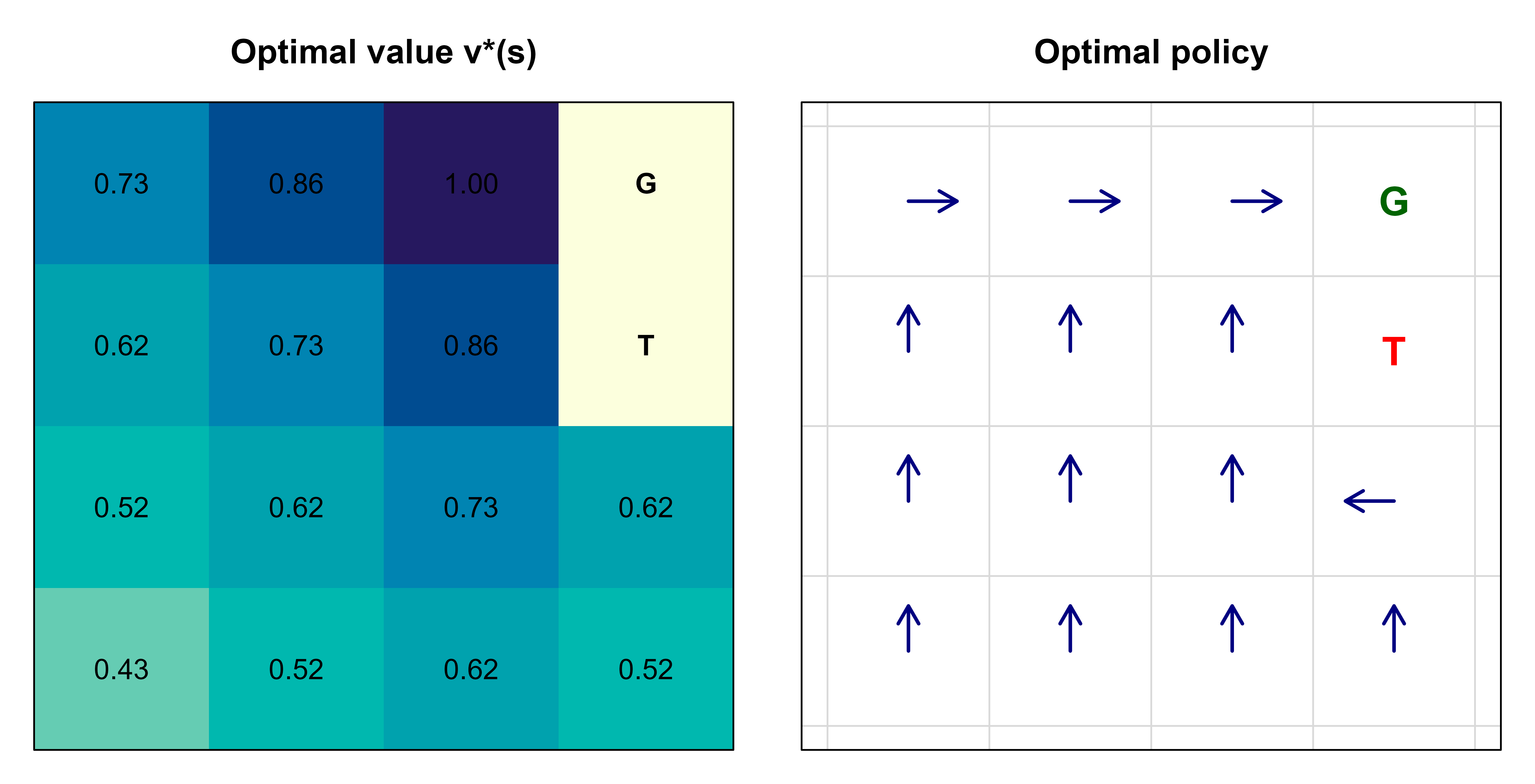
Finally we visualize both the value surface and the greedy policy. Figure 64.1 shows, on the left, a heatmap of \(v_*\) where brighter cells are more valuable, and on the right, the optimal policy as arrows pointing in the chosen direction from each non-terminal cell. The two panels share a single label because they are drawn in one chunk with par(mfrow).

op <- par(mfrow = c(1, 2), mar = c(1, 1, 3, 1))

# ---- Left panel: value heatmap ----
# image() plots column-major with y increasing upward, so flip rows to put
# grid row 1 at the top of the figure.
vmat <- matrix(vi$V, nrow = n_rows, ncol = n_cols, byrow = TRUE)
vplot <- t(vmat[n_rows:1, ])
cols <- hcl.colors(64, "YlGnBu", rev = TRUE)
image(1:n_cols, 1:n_rows, vplot, col = cols, axes = FALSE,
      xlab = "", ylab = "", main = "Optimal value v*(s)")
for (s in seq_len(n_states)) {
  rc <- state_to_rc(s)
  x <- rc["col"]; y <- n_rows - rc["row"] + 1L
  tag <- if (s == goal_state) "G" else if (s == trap_state) "T"
         else sprintf("%.2f", vi$V[s])
  text(x, y, tag, cex = 1.0, font = if (s %in% terminal) 2 else 1)
}
box()

# ---- Right panel: greedy policy arrows ----
plot(NA, xlim = c(0.5, n_cols + 0.5), ylim = c(0.5, n_rows + 0.5),
     axes = FALSE, xlab = "", ylab = "", main = "Optimal policy")
arrow_dx <- c(up = 0, down = 0, left = -0.3, right = 0.3)
arrow_dy <- c(up = 0.3, down = -0.3, left = 0, right = 0)
for (s in seq_len(n_states)) {
  rc <- state_to_rc(s)
  x <- rc["col"]; y <- n_rows - rc["row"] + 1L
  if (s == goal_state) { text(x, y, "G", font = 2, cex = 1.4, col = "darkgreen"); next }
  if (s == trap_state) { text(x, y, "T", font = 2, cex = 1.4, col = "red"); next }
  a <- actions[vi_policy[s]]
  arrows(x, y, x + arrow_dx[a], y + arrow_dy[a], length = 0.12, lwd = 2,
         col = "navy")
}
# Light grid lines for orientation.
abline(h = 0.5 + 0:n_rows, col = "gray85")
abline(v = 0.5 + 0:n_cols, col = "gray85")
box()

par(op)

Figure 64.1: Solution to the 4x4 gridworld. Left: heatmap of the optimal state-value function \(v_*\) (brighter is higher value). Right: the optimal greedy policy, with arrows showing the best action in each non-terminal cell, G marking the goal and T the trap. Value increases smoothly toward the goal, and the arrows trace shortest safe paths that steer around the trap.

The picture matches intuition. Value rises as you approach the goal, the trap pushes a basin of low value around cell 8, and the arrows trace the shortest routes to the goal that keep clear of the trap. Both algorithms produced identical policies, which we can confirm directly.

cat("VI and PI greedy policies identical:",
    identical(vi_policy, pi_sol$policy), "\n")
#> VI and PI greedy policies identical: TRUE

64.9 Comparing the two algorithms

Policy iteration and value iteration are two routes to the same fixed point, and the right choice depends on the shape of your problem. Table 64.2 summarizes the trade-offs.

compare <- data.frame(
  Aspect = c("Inner loop",
             "Evaluation per iteration",
             "Cost per iteration",
             "Iterations to converge",
             "Best when"),
  `Policy iteration` = c(
    "Evaluate policy fully, then improve",
    "Solve/iterate to v_pi exactly",
    "Higher (solve or many sweeps)",
    "Few (finite, often 3-10)",
    "Actions are expensive to compare; few distinct policies"),
  `Value iteration` = c(
    "One Bellman optimality sweep",
    "Single backup, no full evaluation",
    "Lower per sweep",
    "More (until value converges)",
    "Large state spaces; cheap per-sweep updates preferred"),
  check.names = FALSE,
  stringsAsFactors = FALSE
)

knitr::kable(
  compare,
  caption = "Policy iteration versus value iteration for solving a known finite MDP. Both converge to the same optimal value function and policy; they differ in how much evaluation work they do between policy improvements.",
  align = "l"
)

Table 64.2: Policy iteration versus value iteration for solving a known finite MDP. Both converge to the same optimal value function and policy; they differ in how much evaluation work they do between policy improvements.

Aspect	Policy iteration	Value iteration
Inner loop	Evaluate policy fully, then improve	One Bellman optimality sweep
Evaluation per iteration	Solve/iterate to v_pi exactly	Single backup, no full evaluation
Cost per iteration	Higher (solve or many sweeps)	Lower per sweep
Iterations to converge	Few (finite, often 3-10)	More (until value converges)
Best when	Actions are expensive to compare; few distinct policies	Large state spaces; cheap per-sweep updates preferred

In practice the two interpolate into a family called generalized policy iteration: any interleaving of partial evaluation and partial improvement converges, with full policy iteration and single-sweep value iteration as the endpoints. Real implementations often run a few evaluation sweeps between improvements, taking the middle of that spectrum.

64.9.1 Computational complexity

A single Bellman backup at one state evaluates \(|\mathcal{A}|\) actions, each summing over successor states, so a full value-iteration sweep costs \(O(|\mathcal{S}|^2 |\mathcal{A}|)\) for a dense transition model and \(O(|\mathcal{S}| |\mathcal{A}| B)\) when each state-action pair has at most \(B\) reachable successors (in the deterministic gridworld \(B = 1\)). Combined with the iteration bound from Equation 64.1, value iteration runs in \(O\!\big(|\mathcal{S}|^2 |\mathcal{A}| \cdot \tfrac{\log(1/\epsilon)}{1 - \gamma}\big)\) to reach \(\epsilon\)-accuracy, using \(\log(1/\gamma) \approx 1 - \gamma\) for \(\gamma\) near 1.

Policy iteration trades more work per iteration for far fewer iterations. Each evaluation by the direct solve costs \(O(|\mathcal{S}|^3)\) (the matrix factorization), plus \(O(|\mathcal{S}|^2 |\mathcal{A}|)\) for the improvement step. The payoff is that the number of policy-improvement steps is typically tiny, on the order of a handful in practice. The known worst-case bounds are striking: the number of iterations of policy iteration is at most the number of deterministic policies \(|\mathcal{A}|^{|\mathcal{S}|}\), but much sharper results hold. For a fixed discount \(\gamma\), Howard’s policy iteration converges in a number of iterations that is strongly polynomial, bounded by \(O\!\big(\tfrac{|\mathcal{S}|^2 |\mathcal{A}|}{1 - \gamma} \log \tfrac{1}{1-\gamma}\big)\) (Ye, 2011), independent of the reward magnitudes. This is why policy iteration usually wins on small to medium MDPs where the \(O(|\mathcal{S}|^3)\) solve is affordable, while value iteration is preferred when \(|\mathcal{S}|\) is large enough that a cubic solve is prohibitive but cheap per-sweep linear backups are not.

Note

The exponential factor \(|\mathcal{A}|^{|\mathcal{S}|}\) is a loose upper bound, not the typical behavior. On almost all problems policy iteration converges in single-digit or low double-digit iterations because each improvement changes the policy at many states at once and the value increases monotonically toward \(v_*\).

64.10 Practical guidance and pitfalls

Several issues bite people the first time they apply this machinery, and most trace back to modeling rather than to the algorithms.

The most common mistake is a non-Markov state. If the agent’s value function looks unstable or a “good” policy behaves erratically, ask whether the state actually summarizes everything predictive of the future. Position without velocity, board state without whose-turn-it-is, or a sensor reading without recent context will all silently violate the Markov property and corrupt the values. The fix is in the state representation, not the solver.

Reward design is the next trap. Because the agent maximizes cumulative reward exactly as specified, any loophole in the reward function will be found and exploited, a phenomenon called reward hacking. Sparse rewards (only \(+1\) at a far-off goal) make learning slow because credit is hard to assign; dense shaping rewards speed things up but can accidentally encode the wrong objective. Keep the reward aligned with the true goal and verify the resulting behavior, not just the reward total.

The discount factor deserves deliberate choice. Values near \(1\) make the agent far-sighted but slow the contraction (convergence rate scales with \(\gamma\)), can produce numerically large values, and stress the matrix solve in policy iteration as \(\mathbf{I} - \gamma \mathbf{P}_\pi\) approaches singularity. Values too small make the agent myopic and may ignore the very long-horizon payoffs you care about. Treat \(\gamma\) as a modeling decision tied to your effective planning horizon, roughly \(1 / (1 - \gamma)\) steps.

Finally, remember the scope of what we did here. Exact dynamic programming requires the full model \(p\) and a state space small enough to sweep. That is rarely true of real problems. When the model is unknown you turn to model-free methods such as Monte Carlo and temporal-difference learning (Chapter 66), including Q-learning; when the state space is too large to enumerate you replace the value table with a function approximator such as a neural network (Chapter 15), which leads into deep reinforcement learning (Chapter 71). The Bellman equations and the value-function vocabulary from this chapter remain the backbone of all of those methods.

When to use this

Use exact dynamic programming when you genuinely know the dynamics and the state space is small (inventory control on a coarse grid, small scheduling problems, textbook MDPs). For anything with an unknown or huge environment, treat this chapter as the conceptual foundation and reach for the sample-based methods in the chapters that follow.

64.11 Further reading

The standard, freely available reference is Sutton and Barto, Reinforcement Learning: An Introduction, 2nd edition (2018); its early chapters cover MDPs, value functions, the Bellman equations, and dynamic programming in depth, and it is the source most of the notation here follows. For the theory of dynamic programming and MDPs, Bellman’s original Dynamic Programming (1957) introduced the principle of optimality, and Puterman’s Markov Decision Processes: Discrete Stochastic Dynamic Programming (1994) is the rigorous mathematical treatment, including convergence proofs for policy and value iteration. Bertsekas, Dynamic Programming and Optimal Control (2017), gives a control-theoretic perspective with careful attention to approximation. For the modern deep-RL extensions referenced above, Mnih et al. (2015) on deep Q-networks and Silver et al. (2016) on AlphaGo are landmark applications that build directly on the foundations in this chapter.

---

1. The exploration/exploitation dilemma is the heart of the multi-armed bandit problem (Chapter 65) and of the contextual bandit chapter (Chapter 72) elsewhere in this book. Dynamic programming sidesteps it entirely by assuming a known model.