Most of this book treats prediction as a question with a single, self-contained answer: given an input, return a number (regression) or a class label (classification). Many real problems are not like that. When you tag the words of a sentence with parts of speech, the answer is a whole sequence of labels, one per word, and the labels are not independent: a determiner is rarely followed by a verb, a noun phrase has internal grammar. When you segment an image into regions, the label of one pixel pulls on its neighbors. When you parse a sentence, the output is a tree. In each case the thing you are predicting has internal shape, and the parts constrain one another. Predicting such objects is called structured prediction.
The naive workaround is to chop the structured output into pieces and predict each piece on its own. Tag each word with an independent classifier; label each pixel by itself. This throws away exactly the information that makes the problem solvable. If “fly” can be a noun or a verb, the word alone will not tell you which; the surrounding tags will. Structured prediction keeps the pieces together and scores whole configurations, so that the prediction for one part can depend on the predictions for the others.
Intuition
A spell-checker that corrects each letter in isolation is hopeless. One that knows which letter sequences form real words, and which word sequences form real sentences, can fix errors a per-letter model cannot even see. Structure is the extra constraint that turns an impossible local decision into an easy global one.
This raises an immediate difficulty. If a sentence has \(T\) words and each word can take one of \(K\) tags, there are \(K^T\) possible taggings. We cannot score them all. The art of structured prediction is to define scores that decompose over small, overlapping pieces of the output, so that the best whole configuration can be found efficiently by dynamic programming even though the number of configurations is astronomical. This chapter develops that idea for the most common and most tractable case, the linear chain, which covers sequence labeling tasks like part-of-speech tagging, named-entity recognition, and gene finding.
We build up in layers. First we set notation and the central computational problem, the search for the highest-scoring output (the argmax or inference problem). Then we cover the three workhorse models that share this computational core but differ in how they are trained: the hidden Markov model seen as a scorer, the conditional random field, the structured perceptron, and the structured support vector machine. The runnable centerpiece is a from-scratch implementation of the Viterbi algorithm, the dynamic program that solves the argmax for a linear chain, applied to a small toy model so you can watch it decode the most likely label sequence.
77.1 Notation and the Scoring View
Fix some notation we will use throughout. The input is a sequence \(x = (x_1, \dots, x_T)\), where \(x_t\) is the observation at position \(t\) (a word, a pixel, a measurement). The output is a label sequence \(y = (y_1, \dots, y_T)\), where each \(y_t\) takes a value in a finite tag set \(\mathcal{S} = \{1, \dots, K\}\). We write \(\mathcal{Y}(x)\) for the set of all valid label sequences for input \(x\); for an unconstrained linear chain this is simply \(\mathcal{S}^T\), all \(K^T\) sequences.
The unifying idea across every model in this chapter is that we assign a real-valued score \(s(x, y)\) to each input-output pair, and predict by choosing the highest-scoring output:
This is the inference or decoding problem. It is the structured analogue of “take the class with the largest predicted probability,” except that the maximization now ranges over an exponentially large set.
The score is built to decompose over local pieces. For a linear chain we assume it factors into per-position terms plus pairwise terms between adjacent labels:
where \(\psi_t(k, x)\) scores “label \(k\) at position \(t\) given the input” (the emission or unary score) and \(\phi(j, k)\) scores the transition from label \(j\) to label \(k\) (the pairwise score). The crucial property is the Markov assumption: a label interacts directly only with its immediate neighbors, never with distant positions except through the chain. This locality is what makes efficient inference possible.
Key idea
Decomposition is everything. Because the score is a sum of terms that each touch at most two adjacent labels, we can find the best whole sequence without enumerating all \(K^T\) of them. The number of sequences is exponential; the work to find the best one is linear in \(T\).
In a linear model, every score is a weighted feature count. Collect all the model parameters into a single weight vector \(w\), and define a feature function \(\mathbf{f}(x, y)\) that counts how often each feature fires across the whole structure. Then
where \(\mathbf{f}_t\) is the vector of local features at position \(t\) (emission features depending on \(y_t\) and \(x\), transition features depending on \(y_{t-1}\) and \(y_t\)). The decomposition of the score is inherited from the decomposition of the features into local pieces. Models differ in how \(w\) is learned, not in this scoring structure, which is why they all share the same Viterbi decoder.
77.2 The Models
77.2.1 Hidden Markov Models as Scorers
The hidden Markov model (HMM) is the classical generative model for sequences. It posits that a hidden label sequence \(y\) is drawn from a Markov chain, and each observation \(x_t\) is generated from its label \(y_t\):
where \(\pi\) is the initial-state distribution, \(A(j,k) = p(y_t=k \mid y_{t-1}=j)\) is the transition matrix, and \(B(k, o) = p(x_t = o \mid y_t = k)\) is the emission matrix. Taking logs turns the product into a sum and reveals an HMM as a special case of the additive score above, with \(\psi_t(k, x) = \log B(k, x_t)\) (plus \(\log \pi(k)\) at \(t=1\)) and \(\phi(j, k) = \log A(j, k)\).
Note
An HMM is a generative model: it describes how \(x\) and \(y\) are jointly produced, and is trained to maximize \(p(x, y)\). The discriminative models below model \(p(y \mid x)\) or just a score, never spending capacity on explaining \(x\). For prediction we only ever need \(p(y \mid x)\), so the generative effort can be wasted, but HMMs are simple, have closed-form maximum-likelihood estimates (just count transitions and emissions), and decode with the very same Viterbi algorithm.
77.2.1.1 The Markov assumptions, made precise
The factorization of \(p(x,y)\) rests on two conditional-independence statements. The first is the order-one Markov property on the hidden chain,
so each observation depends only on its own hidden state. Applying the chain rule of probability and then deleting the variables these assumptions render irrelevant gives the factorization in Equation 77.2 directly:
These are exactly the assumptions that the additive, neighbor-only score of Equation 77.1 encodes, which is why the log-joint is a linear-chain score.
77.2.1.2 Maximum-likelihood estimation from labeled data
When the label sequences are observed in training (the fully supervised case relevant to structured prediction, as opposed to the latent-state case handled by Baum-Welch / EM), the maximum-likelihood estimates are simple normalized counts, and it is worth deriving why. Suppose we have a corpus of labeled sequences. The log-likelihood is, by Equation 77.3,
\[
\ell(\pi, A, B) = \sum_i \Big[ \log \pi(y^{(i)}_1) + \sum_{t\ge 2}\log A(y^{(i)}_{t-1}, y^{(i)}_t) + \sum_{t}\log B(y^{(i)}_t, x^{(i)}_t) \Big].
\]
The parameters live in disjoint groups (each row of \(A\), each row of \(B\), and \(\pi\) is a probability vector), so the objective separates and we maximize each row independently subject to its simplex constraint. Take one transition row \(A(j,\cdot)\). Let \(n_{jk}\) be the number of times the bigram \((j,k)\) occurs in the data. The relevant part of the objective is \(\sum_k n_{jk}\log A(j,k)\) with \(\sum_k A(j,k)=1\). Introduce a Lagrange multiplier \(\nu\):
where \(m_{ko}\) counts emissions of symbol \(o\) from state \(k\) and \(c_k\) counts sequences that start in state \(k\). The same Lagrangian argument is the multinomial MLE used throughout the book; it reappears below as the stationary condition of the CRF gradient. In practice one adds pseudo-counts (Laplace / Dirichlet smoothing) to avoid zeros, which corresponds to MAP estimation under a Dirichlet prior.
77.2.1.3 The forward algorithm and the data likelihood
Decoding uses the max-product recursion (Viterbi). The companion sum-product recursion, the forward algorithm, computes the marginal likelihood \(p(x) = \sum_y p(x,y)\), which is needed for model comparison and is the HMM precursor of the CRF partition function. Define the forward variable \(\alpha_t(k) = p(x_{1:t}, y_t = k)\). Conditioning on the previous state and using both Markov assumptions,
This is identical in shape to Viterbi (Equation 77.12) with the \(\max\) replaced by a \(\sum\), the manifestation of a single semiring template (max-plus for decoding, sum-product for likelihood) underlying both. It runs in the same \(O(TK^2)\) time.
Note
The MLE in Equation 77.4 is consistent: as the number of labeled sequences grows, \(\hat A, \hat B, \hat\pi\) converge to the true parameters at the standard \(O_p(n^{-1/2})\) rate, because each is a smooth function of sample frequencies. What an HMM cannot fix is misspecification: if the emission-independence assumption is false (observations carry correlated, overlapping features), no amount of data recovers a model the family does not contain. This is the structural reason discriminative CRFs, which never commit to a generative story for \(x\), often win in practice.
77.2.2 Conditional Random Fields
A conditional random field (CRF) models the conditional distribution directly. The linear-chain CRF defines
where the partition function \(Z(x) = \sum_{y' \in \mathcal{Y}(x)} \exp(s(x, y'))\) normalizes over all sequences. The exponential family form means CRFs are the structured generalization of multinomial logistic regression: replace “softmax over \(K\) classes” with “softmax over \(K^T\) sequences.”
Training maximizes the conditional log-likelihood over a labeled corpus \(\{(x^{(i)}, y^{(i)})\}\), usually with an \(\ell_2\) penalty:
where the expectation is computed with the forward-backward algorithm (the sum-product analogue of Viterbi). At the optimum, model expectations match empirical counts. The two hard quantities, \(Z(x)\) and the feature expectations, are both computable in \(O(T K^2)\) time by dynamic programming, the same complexity as decoding.
77.2.2.1 Deriving the gradient
The gradient form is not magic; it is the generic identity for an exponential family. Write the per-example conditional log-likelihood (drop the \(\ell_2\) term, which contributes \(-\lambda w\) trivially) as \(\ell_i(w) = w^\top \mathbf f(x^{(i)}, y^{(i)}) - \log Z_w(x^{(i)})\). The only nontrivial piece is the gradient of the log-partition function. Differentiating \(\log Z_w(x) = \log \sum_{y'} \exp(w^\top \mathbf f(x,y'))\),
So the log-partition function is the cumulant generating function of the features: its gradient is their mean. Subtracting it from \(\mathbf f(x^{(i)},y^{(i)})\) and summing over examples gives Equation 77.6. The exponentially large expectation in Equation 77.7 does not require enumerating sequences: because the features decompose locally, the expectation reduces to per-position and per-edge marginals \(p_w(y_t=k\mid x)\) and \(p_w(y_{t-1}=j, y_t=k\mid x)\), which forward-backward delivers.
77.2.2.2 Forward-backward for the CRF
Define the (unnormalized) forward and backward variables in the CRF, with \(M_t(j,k) = \exp(\phi(j,k) + \psi_t(k,x))\) the position-\(t\) transition matrix:
Each marginal is a normalized product of “score of all ways to reach here from the left” times “score of all ways to finish from here to the right,” which is exactly what the recursion accumulates. In practice run these in log space with log-sum-exp.
77.2.2.3 Concavity and the Hessian
The objective is concave because \(\log Z_w\) is convex in \(w\). Differentiating Equation 77.7 once more gives the Hessian of \(\log Z_w\) as a covariance matrix,
which is positive semidefinite since any covariance matrix is. Therefore the negative log-likelihood is convex, its sum is convex, and the \(\frac{\lambda}{2}\lVert w\rVert^2\) penalty makes it \(\lambda\)-strongly convex, giving a unique global optimum. There are no spurious local optima to worry about, which is why off-the-shelf L-BFGS or stochastic gradient on the CRF objective is reliable. The price is that each gradient evaluation runs forward-backward on every sequence, \(O(\sum_i T_i K^2)\) per epoch.
Intuition
A CRF is logistic regression that has learned to be polite to its neighbors. The transition scores let it say “I would label this word a verb, but the previous tag makes that unlikely, so I will reconsider,” and it balances all such local pressures into one globally coherent sequence.
77.2.3 The Structured Perceptron
Collins’s structured perceptron dispenses with probabilities entirely. It keeps the linear score \(s(x, y) = w^\top \mathbf{f}(x, y)\) and trains \(w\) by a stunningly simple online rule. For each training example, decode with the current weights, and if the prediction is wrong, nudge the weights toward the correct features and away from the predicted ones:
\[
\hat{y} = \arg\max_{y} w^\top \mathbf{f}(x^{(i)}, y), \qquad
w \leftarrow w + \mathbf{f}(x^{(i)}, y^{(i)}) - \mathbf{f}(x^{(i)}, \hat{y}).
\]
If the prediction is already correct, the two feature vectors cancel and nothing changes. The only structured ingredient is the \(\arg\max\), which is again solved by Viterbi. There is no partition function, no expectation, no gradient of a log-likelihood. In practice one averages the weight vectors across all updates, which dramatically improves generalization and is the standard form.
77.2.3.1 Convergence: the structured mistake bound
Collins’s analysis lifts Novikoff’s classical perceptron theorem to structured outputs, and the proof is short enough to give. Say the data are separable with margin \(\gamma > 0\): there exists a unit weight vector \(u\), \(\lVert u\rVert = 1\), such that for every training example and every wrong output \(y \neq y^{(i)}\),
Assume also a radius bound \(\lVert \mathbf f(x^{(i)}, y^{(i)}) - \mathbf f(x^{(i)}, y)\rVert \le R\) for all \(i\) and all \(y\). Let \(w^{(m)}\) be the weight vector before the \(m\)-th mistake, with \(w^{(1)} = 0\). On a mistake the update is \(w^{(m+1)} = w^{(m)} + \boldsymbol\delta\) with \(\boldsymbol\delta = \mathbf f(x^{(i)}, y^{(i)}) - \mathbf f(x^{(i)}, \hat y)\). Project onto \(u\) and use the margin:
Now bound the norm. Because \(\hat y\) was the decoded (highest-scoring) output, \(w^{(m)\top}\boldsymbol\delta = w^{(m)\top}\mathbf f(x^{(i)},y^{(i)}) - w^{(m)\top}\mathbf f(x^{(i)},\hat y) \le 0\) on a mistake, so
The total number of updates is at most \(R^2/\gamma^2\), independent of the sequence length \(T\), the size of the output space \(K^T\), and the number of examples. Two consequences matter in practice. First, separable data are learned in finitely many passes. Second, the bound depends only on the geometry of the feature differences, so the exponential output space costs nothing in the analysis; it is hidden entirely inside the Viterbi \(\arg\max\). For non-separable data the averaged perceptron, \(\bar w = \frac{1}{NE}\sum_{t=1}^{NE} w^{(t)}\) (where \(w^{(t)}\) is the running weight vector after processing the \(t\)-th example, averaged over all \(N\) examples and \(E\) epochs, not only over mistakes), is the standard fix and enjoys generalization bounds in terms of the number of mistakes a near-optimal separator would make.
Note
The non-negativity step \(w^{(m)\top}\boldsymbol\delta \le 0\) is where exact decoding matters. If Viterbi is replaced by an approximate (for example beam) search, \(\hat y\) need not be the true argmax, the inequality can fail, and the convergence guarantee is lost. This is the structured-prediction face of the general rule that perceptron-style learning assumes an exact inference oracle.
77.2.4 The Structured Support Vector Machine
The structured SVM (Tsochantaridis et al.; Taskar et al.) brings the large-margin principle of the support vector machine (covered in the support vector machines chapter, Chapter 19) to structured outputs. It asks not merely that the correct output score higher than every wrong one, but that it score higher by a margin that grows with how wrong the alternative is. Let \(\Delta(y, y')\) be a loss measuring the discrepancy between two label sequences, for example the Hamming loss \(\sum_t \mathbb{1}[y_t \neq y'_t]\), the number of mislabeled positions. The training objective is
The inner maximization is called loss-augmented inference: find the output that is both high-scoring and far from the truth, the most dangerous competitor. When \(\Delta\) decomposes over positions (as Hamming loss does), the loss-augmented argmax is still a linear-chain argmax and is solved by, once again, Viterbi with the per-position loss folded into the emission scores.
77.2.4.1 From margin constraints to the slack-rescaled QP
The objective above is the unconstrained form. The classical derivation starts from a hard constraint, one per wrong output, and relaxes it with slacks. We ask that the true output beat every alternative by a loss-scaled margin (margin rescaling):
and minimize \(\frac{\lambda}{2}\lVert w\rVert^2 + \frac1n\sum_i \xi_i\). Because the objective increases in \(\xi_i\), at the optimum each slack is as small as the constraints permit, so \(\xi_i\) equals the largest violation:
Taking \(y = y^{(i)}\) inside the inner max contributes \(\Delta(y^{(i)},y^{(i)}) = 0\), so the bracket is always \(\ge 0\) and the outer \(\max(0,\cdot)\) is redundant; substituting back recovers the unconstrained structured hinge exactly. There are \(K^T\) constraints per example, exponentially many, but the cutting-plane and stochastic-subgradient algorithms only ever instantiate the single most-violated one, found by loss-augmented inference, which is why training is tractable.
77.2.4.2 Why this is a sound surrogate
The structured hinge is a convex upper bound on the task loss at the decoder’s prediction, which is what justifies minimizing it. Let \(\hat y = \arg\max_y w^\top\mathbf f(x^{(i)},y)\) be the prediction. Then \(w^\top\mathbf f(x^{(i)},\hat y) \ge w^\top\mathbf f(x^{(i)},y^{(i)})\), so
the right-hand side being the per-example structured hinge. Minimizing the (convex) hinge therefore drives down a genuine upper bound on the (non-convex, discontinuous) structured task loss, the structured analogue of the binary SVM hinge bounding the 0/1 loss.
77.2.4.3 Folding the loss into Viterbi
The loss-augmented argmax \(\max_y\big[w^\top\mathbf f(x^{(i)},y) + \Delta(y^{(i)},y)\big]\) is solvable by Viterbi precisely when \(\Delta\) shares the chain’s locality. For Hamming loss \(\Delta(y^{(i)},y) = \sum_t \mathbb 1[y_t \neq y^{(i)}_t]\), the loss adds a per-position term, so we run ordinary Viterbi (Equation 77.12) on augmented emissions
The transition scores are untouched; only the unary scores gain a reward of \(1\) for each position where the candidate label disagrees with the gold label. The decoder is therefore biased toward exactly the high-scoring-yet-wrong sequences the margin must suppress. Any loss that decomposes over the chain’s cliques (positions and edges) folds in the same way; a loss that does not (for example a sequence-level F-measure) breaks the dynamic program and needs special-purpose inference.
Key idea
CRF, structured perceptron, and structured SVM are three training objectives bolted onto one shared engine. The CRF needs sum-over-sequences (forward-backward); the perceptron and structured SVM need only max-over-sequences (Viterbi). Get the decoder right and you can swap training criteria freely.
library(knitr)compare<-data.frame( Model =c("HMM", "Linear-chain CRF", "Structured perceptron","Structured SVM"), Type =c("Generative", "Discriminative (probabilistic)","Discriminative (non-prob.)", "Discriminative (max-margin)"), `Trained to` =c("max p(x,y)", "max p(y|x)","mistake-driven updates", "max-margin + task loss"), `Inference engine` =c("Viterbi", "Viterbi + forward-backward","Viterbi", "loss-augmented Viterbi"), `Models p(x)?` =c("Yes", "No", "No", "No"), check.names =FALSE)kable(compare, caption ="Linear-chain structured prediction models: all share the Viterbi decoder but differ in training objective and what they model.")
Table 77.1: Linear-chain structured prediction models: all share the Viterbi decoder but differ in training objective and what they model.
Model
Type
Trained to
Inference engine
Models p(x)?
HMM
Generative
max p(x,y)
Viterbi
Yes
Linear-chain CRF
Discriminative (probabilistic)
max p(y|x)
Viterbi + forward-backward
No
Structured perceptron
Discriminative (non-prob.)
mistake-driven updates
Viterbi
No
Structured SVM
Discriminative (max-margin)
max-margin + task loss
loss-augmented Viterbi
No
Table 77.1 shows the common thread: every row decodes with Viterbi, and the discriminative models avoid modeling \(p(x)\), spending their parameters only where prediction needs them.
77.3 The Inference Problem: Viterbi
Everything reduces to solving \(\hat{y} = \arg\max_{y} s(x, y)\) for a linear chain. The Viterbi algorithm is a dynamic program that does this in \(O(T K^2)\) time and \(O(TK)\) space, instead of the \(O(K^T)\) cost of brute force.
The idea is to compute, for each position \(t\) and each candidate label \(k\), the score of the best label prefix that ends in label \(k\) at position \(t\). Call this quantity \(\delta_t(k)\). It obeys a recursion: the best prefix ending in \(k\) at \(t\) extends some best prefix ending in \(j\) at \(t-1\), paying the transition cost \(\phi(j,k)\) and the emission cost \(\psi_t(k, x)\):
We also record which previous label \(j\) achieved each maximum, in a back-pointer table \(\beta_t(k)\). After the forward sweep, the best final label is \(\arg\max_k \delta_T(k)\), and we recover the full sequence by following back-pointers from \(T\) down to \(1\). The maximization over \(j\) is the only place the previous position enters, which is precisely the Markov assumption paying off.
77.3.0.1 Why the recursion is correct
The recursion is a Bellman equation, and its correctness rests on optimal substructure. Define \(\delta_t(k)\) formally as the score of the best length-\(t\) prefix ending in label \(k\),
\[
\delta_t(k) = \max_{y_{1:t-1}} \Big[ \sum_{s=1}^{t}\psi_s(y_s,x) + \sum_{s=2}^{t}\phi(y_{s-1},y_s) \Big]\quad\text{subject to } y_t = k.
\]
We prove Equation 77.12 by induction. The base case \(\delta_1(k)=\psi_1(k,x)\) is immediate. For the inductive step, group the maximization over \(y_{1:t-1}\) by the value \(j\) of the second-to-last label \(y_{t-1}\). The objective splits into a part touching only \(y_{1:t-1}\) and a part touching only the final edge and node, because the score is a sum of terms each local to at most one edge:
\[
\delta_t(k) = \psi_t(k,x) + \max_{j}\Big[ \phi(j,k) + \underbrace{\max_{y_{1:t-2}}\big(\text{score of prefix ending in }j\text{ at }t-1\big)}_{=\,\delta_{t-1}(j)} \Big].
\]
The inner maximum is \(\delta_{t-1}(j)\) by the induction hypothesis, which is legitimate precisely because, once \(y_{t-1}=j\) is fixed, no term in the prefix score depends on \(y_t\) or beyond; the Markov structure decouples the past from the future given the present label. This is the substructure property: an optimal length-\(t\) path must extend an optimal length-\((t-1)\) path to its penultimate state. Brute force re-optimizes the shared prefixes once per full path, doing \(O(K^T)\) work; Viterbi memoizes them, paying \(K\) states \(\times\)\(K\) predecessors \(\times\)\(T\) positions, hence \(O(TK^2)\). The back-pointer \(\beta_t(k) = \arg\max_j[\delta_{t-1}(j)+\phi(j,k)]\) records the maximizing predecessor so the argmax sequence, not just its score, can be reconstructed.
Warning
Run Viterbi in log space, adding log-probabilities, never multiplying raw probabilities. For a sequence of length \(T\), a product of \(T\) probabilities underflows to zero in floating point well before \(T\) gets large, and the algorithm silently returns garbage. Sums of logs are numerically stable.
77.3.1 A Runnable Viterbi Decoder
We now implement Viterbi from scratch in base R and decode a toy weather example, the textbook “ice cream” style HMM. The hidden labels are weather states, Hot and Cold. The observations are the number of ice creams a person ate that day (1, 2, or 3). Hot days tend to produce more ice cream; weather is sticky, so a hot day tends to follow a hot day. We define the model in log space and decode an observation sequence.
Show code
# --- Toy HMM specification (a linear-chain scorer) ---states<-c("Hot", "Cold")obs_alphabet<-c("1", "2", "3")# ice creams eaten# Initial-state distribution pi(state)pi0<-c(Hot =0.6, Cold =0.4)# Transition matrix A[j, k] = P(next = k | current = j); weather is stickyA<-matrix(c(0.7, 0.3,0.4, 0.6), nrow =2, byrow =TRUE, dimnames =list(from =states, to =states))# Emission matrix B[k, o] = P(observe o | state = k)B<-matrix(c(0.2, 0.4, 0.4, # Hot: more ice cream0.5, 0.4, 0.1), # Cold: less ice cream nrow =2, byrow =TRUE, dimnames =list(state =states, obs =obs_alphabet))# --- Viterbi decoder, working entirely in log space ---viterbi<-function(obs, states, pi0, A, B){Tlen<-length(obs)K<-length(states)logpi<-log(pi0)logA<-log(A)logB<-log(B)delta<-matrix(-Inf, nrow =Tlen, ncol =K, dimnames =list(t =seq_len(Tlen), state =states))back<-matrix(0L, nrow =Tlen, ncol =K, dimnames =list(t =seq_len(Tlen), state =states))# Initialization: best prefix of length 1 ending in each statedelta[1, ]<-logpi+logB[, obs[1]]# Recursion: best prefix ending in state k at time tfor(tin2:Tlen){for(kin1:K){scores<-delta[t-1, ]+logA[, k]# extend each predecessor j -> kback[t, k]<-which.max(scores)# remember the best predecessordelta[t, k]<-max(scores)+logB[k, obs[t]]}}# Termination + backtracepath<-integer(Tlen)path[Tlen]<-which.max(delta[Tlen, ])for(tinseq(Tlen-1, 1)){path[t]<-back[t+1, path[t+1]]}best_logprob<-max(delta[Tlen, ])list(path =states[path], log_prob =best_logprob, delta =delta)}# Decode an observed ice-cream sequenceobserved<-c("3", "3", "1", "1", "2", "3", "3")result<-viterbi(observed, states, pi0, A, B)data.frame(day =seq_along(observed), ice_creams =observed, decoded_weather =result$path)#> day ice_creams decoded_weather#> 1 1 3 Hot#> 2 2 3 Hot#> 3 3 1 Cold#> 4 4 1 Cold#> 5 5 2 Hot#> 6 6 3 Hot#> 7 7 3 Hotcat(sprintf("Log-probability of best path: %.3f\n", result$log_prob))#> Log-probability of best path: -10.180
The decoder reads the streak of high ice-cream days as hot weather and the dip at days 3 and 4 as a cold spell, then a return to hot. Notice that a single low-ice-cream day in the middle of a hot streak need not flip the state: the sticky transition score can outvote one weak emission, which is exactly the neighbor-awareness that an independent per-day classifier lacks.
Note
To turn this HMM decoder into a CRF decoder, replace logpi + logB[, obs[1]] and logB[k, obs[t]] with arbitrary emission scores \(\psi_t(k, x)\) and replace logA with arbitrary transition scores \(\phi(j, k)\). The control flow is identical; only the source of the numbers changes. That is the sense in which Viterbi is the shared engine.
77.3.2 Watching the Trellis
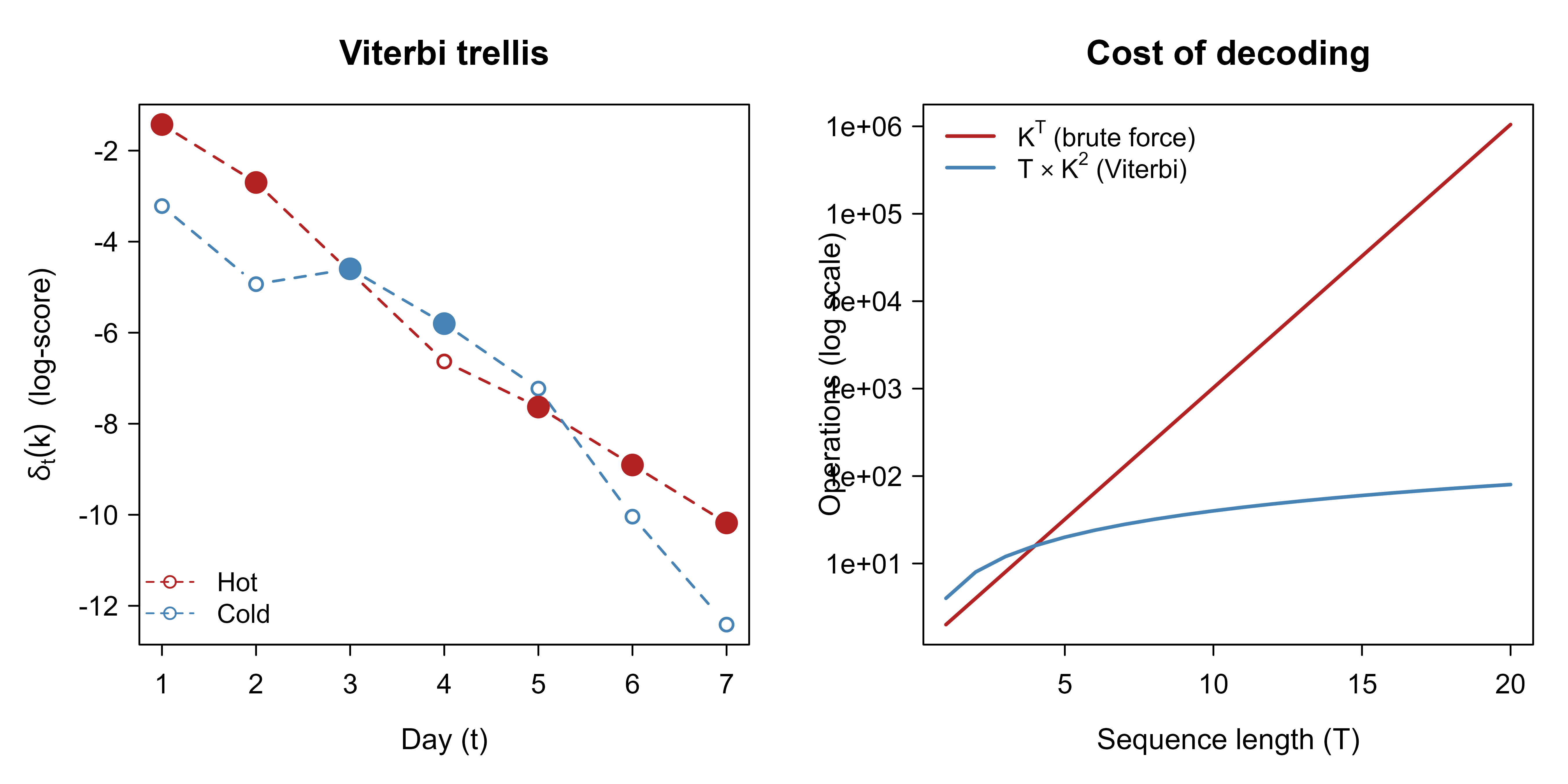
To see why Viterbi avoids exponential work, it helps to picture the trellis: at each time step there is one node per state, and the algorithm keeps a single best-score-so-far per node rather than tracking whole paths. Figure 77.1 plots the running best log-score \(\delta_t(k)\) for each state across the sequence, with the decoded path highlighted, and beside it the brute-force cost it sidesteps.
Show code
op<-par(mfrow =c(1, 2), mar =c(4, 4, 3, 1))# --- Panel 1: the trellis of accumulated best log-scores ---delta<-result$deltaTlen<-nrow(delta)matplot(seq_len(Tlen), delta, type ="b", pch =1, lty =2, col =c("firebrick", "steelblue"), lwd =1.5, xlab ="Day (t)", ylab =expression(delta[t](k)~" (log-score)"), main ="Viterbi trellis")# Highlight the decoded pathdecoded_idx<-match(result$path, states)for(tinseq_len(Tlen)){col_t<-if(decoded_idx[t]==1)"firebrick"else"steelblue"points(t, delta[t, decoded_idx[t]], pch =19, cex =1.6, col =col_t)}legend("bottomleft", legend =states, col =c("firebrick", "steelblue"), lty =2, pch =1, bty ="n", cex =0.9)# --- Panel 2: exponential brute force vs linear-chain Viterbi ---K<-length(states)Ts<-1:20brute<-K^Tsvit<-Ts*K^2plot(Ts, brute, type ="l", log ="y", col ="firebrick", lwd =2, xlab ="Sequence length (T)", ylab ="Operations (log scale)", main ="Cost of decoding")lines(Ts, vit, col ="steelblue", lwd =2)legend("topleft", legend =c(expression(K^T~"(brute force)"),expression(T%*%K^2~"(Viterbi)")), col =c("firebrick", "steelblue"), lwd =2, bty ="n", cex =0.9)par(op)
Figure 77.1: Left: the Viterbi trellis for the ice-cream sequence; each line is the best accumulated log-score for a state over time, and the filled markers trace the decoded path. Right: brute-force cost K^T versus the linear-chain Viterbi cost T*K^2 as the sequence grows, on a log scale.
Figure 77.1 makes the payoff visible: the brute-force curve (left, exponential) rockets off the top of the log scale while the Viterbi curve stays nearly flat. The trellis panel shows that we never store more than \(K\) numbers per column, no matter how many paths funnel through.
77.3.3 Sanity Check Against Brute Force
For a short sequence we can afford to enumerate all \(K^T\) label sequences and confirm that Viterbi returns the true maximizer. This is the kind of check worth keeping in a test suite for any dynamic program.
Show code
# Score any full label sequence under the same model (log space)score_seq<-function(labels, obs, states, pi0, A, B){idx<-match(labels, states)sc<-log(pi0[idx[1]])+log(B[idx[1], obs[1]])for(tin2:length(obs)){sc<-sc+log(A[idx[t-1], idx[t]])+log(B[idx[t], obs[t]])}unname(sc)}# Enumerate all K^T sequences for a short input and find the bestshort_obs<-c("3", "1", "3")grid<-expand.grid(rep(list(states), length(short_obs)), stringsAsFactors =FALSE)all_scores<-apply(grid, 1, function(lab)score_seq(as.character(lab), short_obs, states, pi0, A, B))brute_best<-as.character(grid[which.max(all_scores), ])vit_short<-viterbi(short_obs, states, pi0, A, B)cat("Brute-force best:", paste(brute_best, collapse =" "), "\n")#> Brute-force best: Hot Hot Hotcat("Viterbi best: ", paste(vit_short$path, collapse =" "), "\n")#> Viterbi best: Hot Hot Hotcat("Scores agree: ",isTRUE(all.equal(max(all_scores), vit_short$log_prob)), "\n")#> Scores agree: TRUE
The two methods return the same sequence and the same score, which is the reassurance we want before trusting the decoder on inputs too long to enumerate.
77.3.4 Verifying the Forward Algorithm and a Marginal
The same enumeration lets us check the sum-product side of the story: the forward recursion of Equation 77.5 should reproduce \(p(x) = \sum_y p(x,y)\), and the forward-backward marginal of Equation 77.8 should match a brute-force posterior \(p(y_t = k \mid x)\). Confirming the algebra on a model small enough to enumerate is the surest guard against an off-by-one in the recursion.
Show code
# Forward algorithm: returns p(x) and the full alpha table (linear space here,# fine for a short toy sequence; use log-sum-exp for real lengths)forward<-function(obs, states, pi0, A, B){Tlen<-length(obs); K<-length(states)alpha<-matrix(0, Tlen, K, dimnames =list(t =seq_len(Tlen), state =states))alpha[1, ]<-pi0*B[, obs[1]]for(tin2:Tlen)for(kin1:K)alpha[t, k]<-(alpha[t-1, ]%*%A[, k])*B[k, obs[t]]list(px =sum(alpha[Tlen, ]), alpha =alpha)}# Backward algorithm for the position marginalsbackward<-function(obs, states, pi0, A, B){Tlen<-length(obs); K<-length(states)beta<-matrix(1, Tlen, K, dimnames =list(t =seq_len(Tlen), state =states))for(tinseq(Tlen-1, 1))for(jin1:K)beta[t, j]<-sum(A[j, ]*B[, obs[t+1]]*beta[t+1, ])beta}short_obs<-c("3", "1", "3")# Brute-force p(x) by summing exp(score) over all K^T label sequencesgrid<-expand.grid(rep(list(states), length(short_obs)), stringsAsFactors =FALSE)joint<-apply(grid, 1, function(lab)exp(score_seq(as.character(lab), short_obs, states, pi0, A, B)))px_brute<-sum(joint)fb<-forward(short_obs, states, pi0, A, B)cat(sprintf("p(x): forward = %.6f, brute force = %.6f, agree = %s\n",fb$px, px_brute, isTRUE(all.equal(fb$px, px_brute))))#> p(x): forward = 0.021968, brute force = 0.021968, agree = TRUE# Marginal p(y_2 = Hot | x): forward-backward vs brute forcebw<-backward(short_obs, states, pi0, A, B)marg_fb<-(fb$alpha[2, "Hot"]*bw[2, "Hot"])/fb$pxmarg_bf<-sum(joint[grid$Var2=="Hot"])/px_brutecat(sprintf("p(y2 = Hot | x): forward-backward = %.6f, brute = %.6f, agree = %s\n",marg_fb, marg_bf, isTRUE(all.equal(marg_fb, marg_bf))))#> p(y2 = Hot | x): forward-backward = 0.519301, brute = 0.519301, agree = TRUE
Both the likelihood and the position marginal match the brute-force sums, confirming that the forward recursion and the \(\alpha_t(k)\beta_t(k)/Z\) marginal formula are implemented correctly. These are exactly the quantities a CRF needs for its gradient (Equation 77.6), now validated on a model where we can check every number.
77.4 Practical Guidance and Pitfalls
A few hard-won lessons separate a structured predictor that works from one that quietly underperforms.
Always decode in log space. As the warning above stressed, multiplying probabilities underflows. Add logs. For computing the partition function and expectations in a CRF, use the log-sum-exp trick (subtract the row maximum before exponentiating) to stay stable.
Features are where the accuracy lives. For a CRF or structured perceptron, the model is only as good as \(\mathbf{f}(x, y)\). Rich emission features (word identity, prefixes and suffixes, capitalization, neighboring words, gazetteer membership) typically matter far more than the choice between CRF and structured SVM. Spend your effort there.
Pick the training objective to match your needs. Use a CRF when you need calibrated probabilities (see the probability calibration chapter, Chapter 86) or marginal confidences per position. Use the structured perceptron when you want something dead simple and fast that only needs the argmax. Use the structured SVM when a structured task loss (not plain accuracy) is what you will be judged on, since it optimizes that loss directly through loss-augmented inference.
Label-bias is a real trap. The older maximum-entropy Markov model (MEMM) normalizes transitions locally, per position, which lets states with few outgoing transitions ignore the observation, the label-bias problem. Linear-chain CRFs normalize globally over the whole sequence and avoid it. If you find a per-position normalized model behaving strangely, suspect label bias.
Mind the inference budget. Viterbi is \(O(TK^2)\). With a large tag set \(K\) (hundreds of named-entity types, thousands of words in a language model) the \(K^2\) term dominates and you need pruning (beam search) or structured tag sets. Higher-order chains (depending on the previous \(m\) labels) cost \(O(TK^{m+1})\), so order grows expensive fast.
Beyond chains, exact inference can be intractable. Viterbi exploits the chain. For general graphs (grids in image segmentation, loopy CRFs) exact argmax is NP-hard, and you fall back on approximate inference: loopy belief propagation, graph cuts for certain energy forms, or LP relaxations. Trees still admit exact dynamic programming.
Class and label imbalance still bite, the same difficulty studied in the class imbalance chapter (Chapter 80). Rare tags (a sparse entity type) can be swamped. Position-decomposable losses like weighted Hamming loss, plumbed through the structured SVM’s loss-augmented inference, are a clean way to upweight what you care about.
When to use this
Reach for structured prediction whenever the output is a sequence, segmentation, alignment, or tree whose parts constrain each other, and when a per-part classifier visibly ignores obvious consistency. If the parts really are independent, the extra machinery buys nothing; predict them separately.
A closing perspective: the linear-chain models here are the foundation, not the frontier. Modern sequence labelers usually compute the emission scores \(\psi_t(k, x)\) with a neural network (a BiLSTM or a transformer encoder, see the attention and transformers chapter, Chapter 38) and then place a CRF layer on top to enforce label consistency, decoded with the very Viterbi algorithm implemented above. The dynamic program has outlived every change in how the scores are produced.
77.5 Further Reading
Lafferty, McCallum, and Pereira (2001) introduced conditional random fields and articulated the label-bias problem that motivates global normalization.
Sutton and McCallum (2012), “An Introduction to Conditional Random Fields,” is a thorough and readable monograph on CRFs and their inference.
Collins (2002) introduced the structured (averaged) perceptron for sequence labeling and proved convergence and generalization bounds.
Tsochantaridis, Joachims, Hofmann, and Altun (2005) developed structured support vector machines for interdependent and structured output spaces.
Taskar, Guestrin, and Koller (2003) presented max-margin Markov networks, the large-margin view of structured prediction.
Rabiner (1989) is the classic tutorial on hidden Markov models, including the Viterbi and forward-backward algorithms.
Viterbi (1967) is the original paper on the decoding algorithm, framed for convolutional codes.
Koller and Friedman (2009), “Probabilistic Graphical Models,” gives the general theory of inference in graphical models, of which linear-chain inference is a special case.
Smith (2011), “Linguistic Structure Prediction,” surveys structured prediction with an emphasis on natural language applications.
Source Code
# Structured Prediction {#sec-structured-prediction}```{r}#| include: falsesource("_common.R")```Most of this book treats prediction as a question with a single, self-contained answer: given an input, return a number (regression) or a class label (classification). Many real problems are not like that. When you tag the words of a sentence with parts of speech, the answer is a whole sequence of labels, one per word, and the labels are not independent: a determiner is rarely followed by a verb, a noun phrase has internal grammar. When you segment an image into regions, the label of one pixel pulls on its neighbors. When you parse a sentence, the output is a tree. In each case the thing you are predicting has internal shape, and the parts constrain one another. Predicting such objects is called structured prediction.The naive workaround is to chop the structured output into pieces and predict each piece on its own. Tag each word with an independent classifier; label each pixel by itself. This throws away exactly the information that makes the problem solvable. If "fly" can be a noun or a verb, the word alone will not tell you which; the surrounding tags will. Structured prediction keeps the pieces together and scores whole configurations, so that the prediction for one part can depend on the predictions for the others.::: {.callout-tip title="Intuition"}A spell-checker that corrects each letter in isolation is hopeless. One that knows which letter sequences form real words, and which word sequences form real sentences, can fix errors a per-letter model cannot even see. Structure is the extra constraint that turns an impossible local decision into an easy global one.:::This raises an immediate difficulty. If a sentence has $T$ words and each word can take one of $K$ tags, there are $K^T$ possible taggings. We cannot score them all. The art of structured prediction is to define scores that decompose over small, overlapping pieces of the output, so that the best whole configuration can be found efficiently by dynamic programming even though the number of configurations is astronomical. This chapter develops that idea for the most common and most tractable case, the linear chain, which covers sequence labeling tasks like part-of-speech tagging, named-entity recognition, and gene finding.We build up in layers. First we set notation and the central computational problem, the search for the highest-scoring output (the argmax or inference problem). Then we cover the three workhorse models that share this computational core but differ in how they are trained: the hidden Markov model seen as a scorer, the conditional random field, the structured perceptron, and the structured support vector machine. The runnable centerpiece is a from-scratch implementation of the Viterbi algorithm, the dynamic program that solves the argmax for a linear chain, applied to a small toy model so you can watch it decode the most likely label sequence.## Notation and the Scoring ViewFix some notation we will use throughout. The input is a sequence $x = (x_1, \dots, x_T)$, where $x_t$ is the observation at position $t$ (a word, a pixel, a measurement). The output is a label sequence $y = (y_1, \dots, y_T)$, where each $y_t$ takes a value in a finite tag set $\mathcal{S} = \{1, \dots, K\}$. We write $\mathcal{Y}(x)$ for the set of all valid label sequences for input $x$; for an unconstrained linear chain this is simply $\mathcal{S}^T$, all $K^T$ sequences.The unifying idea across every model in this chapter is that we assign a real-valued score $s(x, y)$ to each input-output pair, and predict by choosing the highest-scoring output:$$\hat{y} = \arg\max_{y \in \mathcal{Y}(x)} s(x, y).$$This is the inference or decoding problem. It is the structured analogue of "take the class with the largest predicted probability," except that the maximization now ranges over an exponentially large set.The score is built to decompose over local pieces. For a linear chain we assume it factors into per-position terms plus pairwise terms between adjacent labels:$$s(x, y) = \sum_{t=1}^{T} \psi_t(y_t, x) \;+\; \sum_{t=2}^{T} \phi(y_{t-1}, y_t),$$ {#eq-structured-prediction-score}where $\psi_t(k, x)$ scores "label $k$ at position $t$ given the input" (the emission or unary score) and $\phi(j, k)$ scores the transition from label $j$ to label $k$ (the pairwise score). The crucial property is the Markov assumption: a label interacts directly only with its immediate neighbors, never with distant positions except through the chain. This locality is what makes efficient inference possible.::: {.callout-important title="Key idea"}Decomposition is everything. Because the score is a sum of terms that each touch at most two adjacent labels, we can find the best whole sequence without enumerating all $K^T$ of them. The number of sequences is exponential; the work to find the best one is linear in $T$.:::In a linear model, every score is a weighted feature count. Collect all the model parameters into a single weight vector $w$, and define a feature function $\mathbf{f}(x, y)$ that counts how often each feature fires across the whole structure. Then$$s(x, y) = w^\top \mathbf{f}(x, y) = \sum_{t} w^\top \mathbf{f}_t(y_{t-1}, y_t, x, t),$$where $\mathbf{f}_t$ is the vector of local features at position $t$ (emission features depending on $y_t$ and $x$, transition features depending on $y_{t-1}$ and $y_t$). The decomposition of the score is inherited from the decomposition of the features into local pieces. Models differ in how $w$ is learned, not in this scoring structure, which is why they all share the same Viterbi decoder.## The Models### Hidden Markov Models as ScorersThe hidden Markov model (HMM) is the classical generative model for sequences. It posits that a hidden label sequence $y$ is drawn from a Markov chain, and each observation $x_t$ is generated from its label $y_t$:$$p(x, y) = \pi(y_1) \prod_{t=2}^{T} A(y_{t-1}, y_t) \prod_{t=1}^{T} B(y_t, x_t),$$ {#eq-structured-prediction-hmm-joint}where $\pi$ is the initial-state distribution, $A(j,k) = p(y_t=k \mid y_{t-1}=j)$ is the transition matrix, and $B(k, o) = p(x_t = o \mid y_t = k)$ is the emission matrix. Taking logs turns the product into a sum and reveals an HMM as a special case of the additive score above, with $\psi_t(k, x) = \log B(k, x_t)$ (plus $\log \pi(k)$ at $t=1$) and $\phi(j, k) = \log A(j, k)$.::: {.callout-note}An HMM is a *generative* model: it describes how $x$ and $y$ are jointly produced, and is trained to maximize $p(x, y)$. The discriminative models below model $p(y \mid x)$ or just a score, never spending capacity on explaining $x$. For prediction we only ever need $p(y \mid x)$, so the generative effort can be wasted, but HMMs are simple, have closed-form maximum-likelihood estimates (just count transitions and emissions), and decode with the very same Viterbi algorithm.:::#### The Markov assumptions, made preciseThe factorization of $p(x,y)$ rests on two conditional-independence statements. The first is the order-one Markov property on the hidden chain,$$p(y_t \mid y_1, \dots, y_{t-1}) = p(y_t \mid y_{t-1}),$$so the future of the chain is independent of its past given the present state. The second is the emission (output) independence,$$p(x_t \mid y_1,\dots,y_T, x_{1:t-1}, x_{t+1:T}) = p(x_t \mid y_t),$$so each observation depends only on its own hidden state. Applying the chain rule of probability and then deleting the variables these assumptions render irrelevant gives the factorization in @eq-structured-prediction-hmm-joint directly:$$p(x,y) = p(y_1)\prod_{t=2}^T p(y_t\mid y_{t-1}) \prod_{t=1}^T p(x_t \mid y_t) = \pi(y_1)\prod_{t=2}^T A(y_{t-1},y_t)\prod_{t=1}^T B(y_t,x_t).$$ {#eq-structured-prediction-hmm-joint-derived}These are exactly the assumptions that the additive, neighbor-only score of @eq-structured-prediction-score encodes, which is why the log-joint is a linear-chain score.#### Maximum-likelihood estimation from labeled dataWhen the label sequences are observed in training (the fully supervised case relevant to structured prediction, as opposed to the latent-state case handled by Baum-Welch / EM), the maximum-likelihood estimates are simple normalized counts, and it is worth deriving why. Suppose we have a corpus of labeled sequences. The log-likelihood is, by @eq-structured-prediction-hmm-joint-derived,$$\ell(\pi, A, B) = \sum_i \Big[ \log \pi(y^{(i)}_1) + \sum_{t\ge 2}\log A(y^{(i)}_{t-1}, y^{(i)}_t) + \sum_{t}\log B(y^{(i)}_t, x^{(i)}_t) \Big].$$The parameters live in disjoint groups (each row of $A$, each row of $B$, and $\pi$ is a probability vector), so the objective separates and we maximize each row independently subject to its simplex constraint. Take one transition row $A(j,\cdot)$. Let $n_{jk}$ be the number of times the bigram $(j,k)$ occurs in the data. The relevant part of the objective is $\sum_k n_{jk}\log A(j,k)$ with $\sum_k A(j,k)=1$. Introduce a Lagrange multiplier $\nu$:$$\mathcal{L} = \sum_k n_{jk}\log A(j,k) - \nu\Big(\sum_k A(j,k) - 1\Big), \qquad\frac{\partial \mathcal{L}}{\partial A(j,k)} = \frac{n_{jk}}{A(j,k)} - \nu = 0.$$Hence $A(j,k) \propto n_{jk}$, and normalizing gives the closed form$$\hat A(j,k) = \frac{n_{jk}}{\sum_{k'} n_{jk'}}, \qquad\hat B(k, o) = \frac{m_{ko}}{\sum_{o'} m_{ko'}}, \qquad\hat\pi(k) = \frac{c_k}{\sum_{k'} c_{k'}},$$ {#eq-structured-prediction-hmm-mle}where $m_{ko}$ counts emissions of symbol $o$ from state $k$ and $c_k$ counts sequences that start in state $k$. The same Lagrangian argument is the multinomial MLE used throughout the book; it reappears below as the stationary condition of the CRF gradient. In practice one adds pseudo-counts (Laplace / Dirichlet smoothing) to avoid zeros, which corresponds to MAP estimation under a Dirichlet prior.#### The forward algorithm and the data likelihoodDecoding uses the max-product recursion (Viterbi). The companion sum-product recursion, the forward algorithm, computes the marginal likelihood $p(x) = \sum_y p(x,y)$, which is needed for model comparison and is the HMM precursor of the CRF partition function. Define the forward variable $\alpha_t(k) = p(x_{1:t}, y_t = k)$. Conditioning on the previous state and using both Markov assumptions,$$\alpha_1(k) = \pi(k)B(k,x_1), \qquad\alpha_t(k) = B(k, x_t)\sum_{j} \alpha_{t-1}(j) A(j,k), \qquadp(x) = \sum_k \alpha_T(k).$$ {#eq-structured-prediction-forward}This is identical in shape to Viterbi (@eq-structured-prediction-viterbi) with the $\max$ replaced by a $\sum$, the manifestation of a single semiring template (max-plus for decoding, sum-product for likelihood) underlying both. It runs in the same $O(TK^2)$ time.::: {.callout-note}The MLE in @eq-structured-prediction-hmm-mle is consistent: as the number of labeled sequences grows, $\hat A, \hat B, \hat\pi$ converge to the true parameters at the standard $O_p(n^{-1/2})$ rate, because each is a smooth function of sample frequencies. What an HMM cannot fix is misspecification: if the emission-independence assumption is false (observations carry correlated, overlapping features), no amount of data recovers a model the family does not contain. This is the structural reason discriminative CRFs, which never commit to a generative story for $x$, often win in practice.:::### Conditional Random FieldsA conditional random field (CRF) models the conditional distribution directly. The linear-chain CRF defines$$p(y \mid x) = \frac{1}{Z(x)} \exp\!\big( s(x, y) \big) = \frac{1}{Z(x)} \exp\!\Big( \sum_t \psi_t(y_t, x) + \sum_t \phi(y_{t-1}, y_t) \Big),$$where the partition function $Z(x) = \sum_{y' \in \mathcal{Y}(x)} \exp(s(x, y'))$ normalizes over all sequences. The exponential family form means CRFs are the structured generalization of multinomial logistic regression: replace "softmax over $K$ classes" with "softmax over $K^T$ sequences."Training maximizes the conditional log-likelihood over a labeled corpus $\{(x^{(i)}, y^{(i)})\}$, usually with an $\ell_2$ penalty:$$\max_{w} \; \sum_i \Big[ w^\top \mathbf{f}(x^{(i)}, y^{(i)}) - \log Z_w(x^{(i)}) \Big] - \frac{\lambda}{2}\lVert w \rVert^2.$$This objective is concave, so it has a unique optimum. Its gradient has the elegant form of "observed feature counts minus expected feature counts,"$$\nabla_w = \sum_i \Big[ \mathbf{f}(x^{(i)}, y^{(i)}) - \mathbb{E}_{y \sim p_w(\cdot \mid x^{(i)})}\,\mathbf{f}(x^{(i)}, y) \Big] - \lambda w,$$ {#eq-structured-prediction-crf-grad}where the expectation is computed with the forward-backward algorithm (the sum-product analogue of Viterbi). At the optimum, model expectations match empirical counts. The two hard quantities, $Z(x)$ and the feature expectations, are both computable in $O(T K^2)$ time by dynamic programming, the same complexity as decoding.#### Deriving the gradientThe gradient form is not magic; it is the generic identity for an exponential family. Write the per-example conditional log-likelihood (drop the $\ell_2$ term, which contributes $-\lambda w$ trivially) as $\ell_i(w) = w^\top \mathbf f(x^{(i)}, y^{(i)}) - \log Z_w(x^{(i)})$. The only nontrivial piece is the gradient of the log-partition function. Differentiating $\log Z_w(x) = \log \sum_{y'} \exp(w^\top \mathbf f(x,y'))$,$$\nabla_w \log Z_w(x)= \frac{\sum_{y'} \exp(w^\top \mathbf f(x,y'))\,\mathbf f(x,y')}{\sum_{y'}\exp(w^\top \mathbf f(x,y'))}= \sum_{y'} p_w(y'\mid x)\,\mathbf f(x,y')= \mathbb E_{y\sim p_w(\cdot\mid x)}\,\mathbf f(x,y).$$ {#eq-structured-prediction-logZ-grad}So the log-partition function is the cumulant generating function of the features: its gradient is their mean. Subtracting it from $\mathbf f(x^{(i)},y^{(i)})$ and summing over examples gives @eq-structured-prediction-crf-grad. The exponentially large expectation in @eq-structured-prediction-logZ-grad does not require enumerating sequences: because the features decompose locally, the expectation reduces to per-position and per-edge marginals $p_w(y_t=k\mid x)$ and $p_w(y_{t-1}=j, y_t=k\mid x)$, which forward-backward delivers.#### Forward-backward for the CRFDefine the (unnormalized) forward and backward variables in the CRF, with $M_t(j,k) = \exp(\phi(j,k) + \psi_t(k,x))$ the position-$t$ transition matrix:$$\alpha_1(k) = \exp(\psi_1(k,x)),\quad\alpha_t(k) = \sum_j \alpha_{t-1}(j)\,M_t(j,k),\qquad\beta_T(k)=1,\quad\beta_t(j) = \sum_k M_{t+1}(j,k)\,\beta_{t+1}(k).$$Then $Z(x) = \sum_k \alpha_T(k)$, and the marginals needed for the gradient are$$p_w(y_t = k\mid x) = \frac{\alpha_t(k)\,\beta_t(k)}{Z(x)}, \qquadp_w(y_{t-1}=j, y_t=k\mid x) = \frac{\alpha_{t-1}(j)\,M_t(j,k)\,\beta_t(k)}{Z(x)}.$$ {#eq-structured-prediction-marginals}Each marginal is a normalized product of "score of all ways to reach here from the left" times "score of all ways to finish from here to the right," which is exactly what the recursion accumulates. In practice run these in log space with log-sum-exp.#### Concavity and the HessianThe objective is concave because $\log Z_w$ is convex in $w$. Differentiating @eq-structured-prediction-logZ-grad once more gives the Hessian of $\log Z_w$ as a covariance matrix,$$\nabla^2_w \log Z_w(x) = \mathbb E_{y\sim p_w}\big[\mathbf f \mathbf f^\top\big] - \big(\mathbb E_{y\sim p_w}\mathbf f\big)\big(\mathbb E_{y\sim p_w}\mathbf f\big)^\top = \operatorname{Cov}_{p_w}\!\big(\mathbf f(x,y)\big) \succeq 0,$$ {#eq-structured-prediction-hessian}which is positive semidefinite since any covariance matrix is. Therefore the negative log-likelihood is convex, its sum is convex, and the $\frac{\lambda}{2}\lVert w\rVert^2$ penalty makes it $\lambda$-strongly convex, giving a unique global optimum. There are no spurious local optima to worry about, which is why off-the-shelf L-BFGS or stochastic gradient on the CRF objective is reliable. The price is that each gradient evaluation runs forward-backward on every sequence, $O(\sum_i T_i K^2)$ per epoch.::: {.callout-tip title="Intuition"}A CRF is logistic regression that has learned to be polite to its neighbors. The transition scores let it say "I would label this word a verb, but the previous tag makes that unlikely, so I will reconsider," and it balances all such local pressures into one globally coherent sequence.:::### The Structured PerceptronCollins's structured perceptron dispenses with probabilities entirely. It keeps the linear score $s(x, y) = w^\top \mathbf{f}(x, y)$ and trains $w$ by a stunningly simple online rule. For each training example, decode with the current weights, and if the prediction is wrong, nudge the weights toward the correct features and away from the predicted ones:$$\hat{y} = \arg\max_{y} w^\top \mathbf{f}(x^{(i)}, y), \qquadw \leftarrow w + \mathbf{f}(x^{(i)}, y^{(i)}) - \mathbf{f}(x^{(i)}, \hat{y}).$$If the prediction is already correct, the two feature vectors cancel and nothing changes. The only structured ingredient is the $\arg\max$, which is again solved by Viterbi. There is no partition function, no expectation, no gradient of a log-likelihood. In practice one averages the weight vectors across all updates, which dramatically improves generalization and is the standard form.#### Convergence: the structured mistake boundCollins's analysis lifts Novikoff's classical perceptron theorem to structured outputs, and the proof is short enough to give. Say the data are separable with margin $\gamma > 0$: there exists a unit weight vector $u$, $\lVert u\rVert = 1$, such that for every training example and every wrong output $y \neq y^{(i)}$,$$u^\top \mathbf f(x^{(i)}, y^{(i)}) - u^\top \mathbf f(x^{(i)}, y) \ge \gamma.$$Assume also a radius bound $\lVert \mathbf f(x^{(i)}, y^{(i)}) - \mathbf f(x^{(i)}, y)\rVert \le R$ for all $i$ and all $y$. Let $w^{(m)}$ be the weight vector before the $m$-th mistake, with $w^{(1)} = 0$. On a mistake the update is $w^{(m+1)} = w^{(m)} + \boldsymbol\delta$ with $\boldsymbol\delta = \mathbf f(x^{(i)}, y^{(i)}) - \mathbf f(x^{(i)}, \hat y)$. Project onto $u$ and use the margin:$$u^\top w^{(m+1)} = u^\top w^{(m)} + u^\top \boldsymbol\delta \ge u^\top w^{(m)} + \gamma \;\;\Rightarrow\;\; u^\top w^{(m+1)} \ge m\gamma.$$Now bound the norm. Because $\hat y$ was the decoded (highest-scoring) output, $w^{(m)\top}\boldsymbol\delta = w^{(m)\top}\mathbf f(x^{(i)},y^{(i)}) - w^{(m)\top}\mathbf f(x^{(i)},\hat y) \le 0$ on a mistake, so$$\lVert w^{(m+1)}\rVert^2 = \lVert w^{(m)}\rVert^2 + 2 w^{(m)\top}\boldsymbol\delta + \lVert\boldsymbol\delta\rVert^2 \le \lVert w^{(m)}\rVert^2 + R^2 \;\;\Rightarrow\;\; \lVert w^{(m+1)}\rVert^2 \le m R^2.$$Combine with Cauchy-Schwarz, $u^\top w^{(m+1)} \le \lVert u\rVert\,\lVert w^{(m+1)}\rVert = \lVert w^{(m+1)}\rVert$:$$m\gamma \le u^\top w^{(m+1)} \le \lVert w^{(m+1)}\rVert \le \sqrt{m}\,R \;\;\Rightarrow\;\; m \le \frac{R^2}{\gamma^2}.$$ {#eq-structured-prediction-mistake-bound}The total number of updates is at most $R^2/\gamma^2$, independent of the sequence length $T$, the size of the output space $K^T$, and the number of examples. Two consequences matter in practice. First, separable data are learned in finitely many passes. Second, the bound depends only on the geometry of the feature differences, so the exponential output space costs nothing in the analysis; it is hidden entirely inside the Viterbi $\arg\max$. For non-separable data the averaged perceptron, $\bar w = \frac{1}{NE}\sum_{t=1}^{NE} w^{(t)}$ (where $w^{(t)}$ is the running weight vector after processing the $t$-th example, averaged over all $N$ examples and $E$ epochs, not only over mistakes), is the standard fix and enjoys generalization bounds in terms of the number of mistakes a near-optimal separator would make.::: {.callout-note}The non-negativity step $w^{(m)\top}\boldsymbol\delta \le 0$ is where exact decoding matters. If Viterbi is replaced by an approximate (for example beam) search, $\hat y$ need not be the true argmax, the inequality can fail, and the convergence guarantee is lost. This is the structured-prediction face of the general rule that perceptron-style learning assumes an exact inference oracle.:::### The Structured Support Vector MachineThe structured SVM (Tsochantaridis et al.; Taskar et al.) brings the large-margin principle of the support vector machine (covered in the support vector machines chapter, @sec-svm) to structured outputs. It asks not merely that the correct output score higher than every wrong one, but that it score higher by a margin that grows with how wrong the alternative is. Let $\Delta(y, y')$ be a loss measuring the discrepancy between two label sequences, for example the Hamming loss $\sum_t \mathbb{1}[y_t \neq y'_t]$, the number of mislabeled positions. The training objective is$$\min_{w} \; \frac{\lambda}{2}\lVert w \rVert^2 + \frac{1}{n}\sum_i \max_{y \in \mathcal{Y}(x^{(i)})} \Big[ \Delta(y^{(i)}, y) + w^\top \mathbf{f}(x^{(i)}, y) - w^\top \mathbf{f}(x^{(i)}, y^{(i)}) \Big].$$The inner maximization is called loss-augmented inference: find the output that is both high-scoring and far from the truth, the most dangerous competitor. When $\Delta$ decomposes over positions (as Hamming loss does), the loss-augmented argmax is still a linear-chain argmax and is solved by, once again, Viterbi with the per-position loss folded into the emission scores.#### From margin constraints to the slack-rescaled QPThe objective above is the unconstrained form. The classical derivation starts from a hard constraint, one per wrong output, and relaxes it with slacks. We ask that the true output beat every alternative by a loss-scaled margin (margin rescaling):$$w^\top \mathbf f(x^{(i)}, y^{(i)}) - w^\top \mathbf f(x^{(i)}, y) \ge \Delta(y^{(i)}, y) - \xi_i \quad \forall y \in \mathcal Y(x^{(i)}),\qquad \xi_i \ge 0,$$and minimize $\frac{\lambda}{2}\lVert w\rVert^2 + \frac1n\sum_i \xi_i$. Because the objective increases in $\xi_i$, at the optimum each slack is as small as the constraints permit, so $\xi_i$ equals the largest violation:$$\xi_i = \max\Big(0,\; \max_{y}\big[\Delta(y^{(i)},y) + w^\top\mathbf f(x^{(i)},y)\big] - w^\top\mathbf f(x^{(i)},y^{(i)})\Big).$$Taking $y = y^{(i)}$ inside the inner max contributes $\Delta(y^{(i)},y^{(i)}) = 0$, so the bracket is always $\ge 0$ and the outer $\max(0,\cdot)$ is redundant; substituting back recovers the unconstrained structured hinge exactly. There are $K^T$ constraints per example, exponentially many, but the cutting-plane and stochastic-subgradient algorithms only ever instantiate the single most-violated one, found by loss-augmented inference, which is why training is tractable.#### Why this is a sound surrogateThe structured hinge is a convex upper bound on the task loss at the decoder's prediction, which is what justifies minimizing it. Let $\hat y = \arg\max_y w^\top\mathbf f(x^{(i)},y)$ be the prediction. Then $w^\top\mathbf f(x^{(i)},\hat y) \ge w^\top\mathbf f(x^{(i)},y^{(i)})$, so$$\Delta(y^{(i)},\hat y) \le \Delta(y^{(i)},\hat y) + \big[w^\top\mathbf f(x^{(i)},\hat y) - w^\top\mathbf f(x^{(i)},y^{(i)})\big] \le \max_y\big[\Delta(y^{(i)},y) + w^\top\mathbf f(x^{(i)},y) - w^\top\mathbf f(x^{(i)},y^{(i)})\big],$$ {#eq-structured-prediction-ssvm-bound}the right-hand side being the per-example structured hinge. Minimizing the (convex) hinge therefore drives down a genuine upper bound on the (non-convex, discontinuous) structured task loss, the structured analogue of the binary SVM hinge bounding the 0/1 loss.#### Folding the loss into ViterbiThe loss-augmented argmax $\max_y\big[w^\top\mathbf f(x^{(i)},y) + \Delta(y^{(i)},y)\big]$ is solvable by Viterbi precisely when $\Delta$ shares the chain's locality. For Hamming loss $\Delta(y^{(i)},y) = \sum_t \mathbb 1[y_t \neq y^{(i)}_t]$, the loss adds a per-position term, so we run ordinary Viterbi (@eq-structured-prediction-viterbi) on augmented emissions$$\tilde\psi_t(k, x) = \psi_t(k,x) + \mathbb 1[k \neq y^{(i)}_t].$$The transition scores are untouched; only the unary scores gain a reward of $1$ for each position where the candidate label disagrees with the gold label. The decoder is therefore biased toward exactly the high-scoring-yet-wrong sequences the margin must suppress. Any loss that decomposes over the chain's cliques (positions and edges) folds in the same way; a loss that does not (for example a sequence-level F-measure) breaks the dynamic program and needs special-purpose inference.::: {.callout-important title="Key idea"}CRF, structured perceptron, and structured SVM are three training objectives bolted onto one shared engine. The CRF needs sum-over-sequences (forward-backward); the perceptron and structured SVM need only max-over-sequences (Viterbi). Get the decoder right and you can swap training criteria freely.:::@tbl-structured-prediction-model-compare lays out how these models relate.```{r tbl-structured-prediction-model-compare}library(knitr)compare <-data.frame(Model =c("HMM", "Linear-chain CRF", "Structured perceptron","Structured SVM"),Type =c("Generative", "Discriminative (probabilistic)","Discriminative (non-prob.)", "Discriminative (max-margin)"),`Trained to`=c("max p(x,y)", "max p(y|x)","mistake-driven updates", "max-margin + task loss"),`Inference engine`=c("Viterbi", "Viterbi + forward-backward","Viterbi", "loss-augmented Viterbi"),`Models p(x)?`=c("Yes", "No", "No", "No"),check.names =FALSE)kable(compare,caption ="Linear-chain structured prediction models: all share the Viterbi decoder but differ in training objective and what they model.")```@tbl-structured-prediction-model-compare shows the common thread: every row decodes with Viterbi, and the discriminative models avoid modeling $p(x)$, spending their parameters only where prediction needs them.## The Inference Problem: ViterbiEverything reduces to solving $\hat{y} = \arg\max_{y} s(x, y)$ for a linear chain. The Viterbi algorithm is a dynamic program that does this in $O(T K^2)$ time and $O(TK)$ space, instead of the $O(K^T)$ cost of brute force.The idea is to compute, for each position $t$ and each candidate label $k$, the score of the best label prefix that ends in label $k$ at position $t$. Call this quantity $\delta_t(k)$. It obeys a recursion: the best prefix ending in $k$ at $t$ extends some best prefix ending in $j$ at $t-1$, paying the transition cost $\phi(j,k)$ and the emission cost $\psi_t(k, x)$:$$\delta_1(k) = \psi_1(k, x), \qquad\delta_t(k) = \psi_t(k, x) + \max_{j \in \mathcal{S}} \big[ \delta_{t-1}(j) + \phi(j, k) \big].$$ {#eq-structured-prediction-viterbi}We also record which previous label $j$ achieved each maximum, in a back-pointer table $\beta_t(k)$. After the forward sweep, the best final label is $\arg\max_k \delta_T(k)$, and we recover the full sequence by following back-pointers from $T$ down to $1$. The maximization over $j$ is the only place the previous position enters, which is precisely the Markov assumption paying off.#### Why the recursion is correctThe recursion is a Bellman equation, and its correctness rests on optimal substructure. Define $\delta_t(k)$ formally as the score of the best length-$t$ prefix ending in label $k$,$$\delta_t(k) = \max_{y_{1:t-1}} \Big[ \sum_{s=1}^{t}\psi_s(y_s,x) + \sum_{s=2}^{t}\phi(y_{s-1},y_s) \Big]\quad\text{subject to } y_t = k.$$We prove @eq-structured-prediction-viterbi by induction. The base case $\delta_1(k)=\psi_1(k,x)$ is immediate. For the inductive step, group the maximization over $y_{1:t-1}$ by the value $j$ of the second-to-last label $y_{t-1}$. The objective splits into a part touching only $y_{1:t-1}$ and a part touching only the final edge and node, because the score is a sum of terms each local to at most one edge:$$\delta_t(k) = \psi_t(k,x) + \max_{j}\Big[ \phi(j,k) + \underbrace{\max_{y_{1:t-2}}\big(\text{score of prefix ending in }j\text{ at }t-1\big)}_{=\,\delta_{t-1}(j)} \Big].$$The inner maximum is $\delta_{t-1}(j)$ by the induction hypothesis, which is legitimate precisely because, once $y_{t-1}=j$ is fixed, no term in the prefix score depends on $y_t$ or beyond; the Markov structure decouples the past from the future given the present label. This is the substructure property: an optimal length-$t$ path must extend an optimal length-$(t-1)$ path to its penultimate state. Brute force re-optimizes the shared prefixes once per full path, doing $O(K^T)$ work; Viterbi memoizes them, paying $K$ states $\times$ $K$ predecessors $\times$ $T$ positions, hence $O(TK^2)$. The back-pointer $\beta_t(k) = \arg\max_j[\delta_{t-1}(j)+\phi(j,k)]$ records the maximizing predecessor so the argmax sequence, not just its score, can be reconstructed.::: {.callout-warning}Run Viterbi in **log space**, adding log-probabilities, never multiplying raw probabilities. For a sequence of length $T$, a product of $T$ probabilities underflows to zero in floating point well before $T$ gets large, and the algorithm silently returns garbage. Sums of logs are numerically stable.:::### A Runnable Viterbi DecoderWe now implement Viterbi from scratch in base R and decode a toy weather example, the textbook "ice cream" style HMM. The hidden labels are weather states, `Hot` and `Cold`. The observations are the number of ice creams a person ate that day (`1`, `2`, or `3`). Hot days tend to produce more ice cream; weather is sticky, so a hot day tends to follow a hot day. We define the model in log space and decode an observation sequence.```{r structured-prediction-viterbi-impl}# --- Toy HMM specification (a linear-chain scorer) ---states <-c("Hot", "Cold")obs_alphabet <-c("1", "2", "3") # ice creams eaten# Initial-state distribution pi(state)pi0 <-c(Hot =0.6, Cold =0.4)# Transition matrix A[j, k] = P(next = k | current = j); weather is stickyA <-matrix(c(0.7, 0.3,0.4, 0.6),nrow =2, byrow =TRUE,dimnames =list(from = states, to = states))# Emission matrix B[k, o] = P(observe o | state = k)B <-matrix(c(0.2, 0.4, 0.4, # Hot: more ice cream0.5, 0.4, 0.1), # Cold: less ice creamnrow =2, byrow =TRUE,dimnames =list(state = states, obs = obs_alphabet))# --- Viterbi decoder, working entirely in log space ---viterbi <-function(obs, states, pi0, A, B) { Tlen <-length(obs) K <-length(states) logpi <-log(pi0) logA <-log(A) logB <-log(B) delta <-matrix(-Inf, nrow = Tlen, ncol = K,dimnames =list(t =seq_len(Tlen), state = states)) back <-matrix(0L, nrow = Tlen, ncol = K,dimnames =list(t =seq_len(Tlen), state = states))# Initialization: best prefix of length 1 ending in each state delta[1, ] <- logpi + logB[, obs[1]]# Recursion: best prefix ending in state k at time tfor (t in2:Tlen) {for (k in1:K) { scores <- delta[t -1, ] + logA[, k] # extend each predecessor j -> k back[t, k] <-which.max(scores) # remember the best predecessor delta[t, k] <-max(scores) + logB[k, obs[t]] } }# Termination + backtrace path <-integer(Tlen) path[Tlen] <-which.max(delta[Tlen, ])for (t inseq(Tlen -1, 1)) { path[t] <- back[t +1, path[t +1]] } best_logprob <-max(delta[Tlen, ])list(path = states[path], log_prob = best_logprob, delta = delta)}# Decode an observed ice-cream sequenceobserved <-c("3", "3", "1", "1", "2", "3", "3")result <-viterbi(observed, states, pi0, A, B)data.frame(day =seq_along(observed),ice_creams = observed,decoded_weather = result$path)cat(sprintf("Log-probability of best path: %.3f\n", result$log_prob))```The decoder reads the streak of high ice-cream days as hot weather and the dip at days 3 and 4 as a cold spell, then a return to hot. Notice that a single low-ice-cream day in the middle of a hot streak need not flip the state: the sticky transition score can outvote one weak emission, which is exactly the neighbor-awareness that an independent per-day classifier lacks.::: {.callout-note}To turn this HMM decoder into a CRF decoder, replace `logpi + logB[, obs[1]]` and `logB[k, obs[t]]` with arbitrary emission scores $\psi_t(k, x)$ and replace `logA` with arbitrary transition scores $\phi(j, k)$. The control flow is identical; only the source of the numbers changes. That is the sense in which Viterbi is the shared engine.:::### Watching the TrellisTo see *why* Viterbi avoids exponential work, it helps to picture the trellis: at each time step there is one node per state, and the algorithm keeps a single best-score-so-far per node rather than tracking whole paths. @fig-structured-prediction-trellis plots the running best log-score $\delta_t(k)$ for each state across the sequence, with the decoded path highlighted, and beside it the brute-force cost it sidesteps.```{r fig-structured-prediction-trellis, fig.width=9, fig.height=4.5, fig.cap="Left: the Viterbi trellis for the ice-cream sequence; each line is the best accumulated log-score for a state over time, and the filled markers trace the decoded path. Right: brute-force cost K^T versus the linear-chain Viterbi cost T*K^2 as the sequence grows, on a log scale."}op <-par(mfrow =c(1, 2), mar =c(4, 4, 3, 1))# --- Panel 1: the trellis of accumulated best log-scores ---delta <- result$deltaTlen <-nrow(delta)matplot(seq_len(Tlen), delta, type ="b", pch =1, lty =2,col =c("firebrick", "steelblue"), lwd =1.5,xlab ="Day (t)", ylab =expression(delta[t](k)~" (log-score)"),main ="Viterbi trellis")# Highlight the decoded pathdecoded_idx <-match(result$path, states)for (t inseq_len(Tlen)) { col_t <-if (decoded_idx[t] ==1) "firebrick"else"steelblue"points(t, delta[t, decoded_idx[t]], pch =19, cex =1.6, col = col_t)}legend("bottomleft", legend = states, col =c("firebrick", "steelblue"),lty =2, pch =1, bty ="n", cex =0.9)# --- Panel 2: exponential brute force vs linear-chain Viterbi ---K <-length(states)Ts <-1:20brute <- K^Tsvit <- Ts * K^2plot(Ts, brute, type ="l", log ="y", col ="firebrick", lwd =2,xlab ="Sequence length (T)", ylab ="Operations (log scale)",main ="Cost of decoding")lines(Ts, vit, col ="steelblue", lwd =2)legend("topleft", legend =c(expression(K^T~"(brute force)"),expression(T %*% K^2~"(Viterbi)")),col =c("firebrick", "steelblue"), lwd =2, bty ="n", cex =0.9)par(op)```@fig-structured-prediction-trellis makes the payoff visible: the brute-force curve (left, exponential) rockets off the top of the log scale while the Viterbi curve stays nearly flat. The trellis panel shows that we never store more than $K$ numbers per column, no matter how many paths funnel through.### Sanity Check Against Brute ForceFor a short sequence we can afford to enumerate all $K^T$ label sequences and confirm that Viterbi returns the true maximizer. This is the kind of check worth keeping in a test suite for any dynamic program.```{r structured-prediction-bruteforce-check}# Score any full label sequence under the same model (log space)score_seq <-function(labels, obs, states, pi0, A, B) { idx <-match(labels, states) sc <-log(pi0[idx[1]]) +log(B[idx[1], obs[1]])for (t in2:length(obs)) { sc <- sc +log(A[idx[t -1], idx[t]]) +log(B[idx[t], obs[t]]) }unname(sc)}# Enumerate all K^T sequences for a short input and find the bestshort_obs <-c("3", "1", "3")grid <-expand.grid(rep(list(states), length(short_obs)),stringsAsFactors =FALSE)all_scores <-apply(grid, 1, function(lab)score_seq(as.character(lab), short_obs, states, pi0, A, B))brute_best <-as.character(grid[which.max(all_scores), ])vit_short <-viterbi(short_obs, states, pi0, A, B)cat("Brute-force best:", paste(brute_best, collapse =" "), "\n")cat("Viterbi best: ", paste(vit_short$path, collapse =" "), "\n")cat("Scores agree: ",isTRUE(all.equal(max(all_scores), vit_short$log_prob)), "\n")```The two methods return the same sequence and the same score, which is the reassurance we want before trusting the decoder on inputs too long to enumerate.### Verifying the Forward Algorithm and a MarginalThe same enumeration lets us check the sum-product side of the story: the forward recursion of @eq-structured-prediction-forward should reproduce $p(x) = \sum_y p(x,y)$, and the forward-backward marginal of @eq-structured-prediction-marginals should match a brute-force posterior $p(y_t = k \mid x)$. Confirming the algebra on a model small enough to enumerate is the surest guard against an off-by-one in the recursion.```{r structured-prediction-forward-check}# Forward algorithm: returns p(x) and the full alpha table (linear space here,# fine for a short toy sequence; use log-sum-exp for real lengths)forward <-function(obs, states, pi0, A, B) { Tlen <-length(obs); K <-length(states) alpha <-matrix(0, Tlen, K, dimnames =list(t =seq_len(Tlen), state = states)) alpha[1, ] <- pi0 * B[, obs[1]]for (t in2:Tlen)for (k in1:K) alpha[t, k] <- (alpha[t -1, ] %*% A[, k]) * B[k, obs[t]]list(px =sum(alpha[Tlen, ]), alpha = alpha)}# Backward algorithm for the position marginalsbackward <-function(obs, states, pi0, A, B) { Tlen <-length(obs); K <-length(states) beta <-matrix(1, Tlen, K, dimnames =list(t =seq_len(Tlen), state = states))for (t inseq(Tlen -1, 1))for (j in1:K) beta[t, j] <-sum(A[j, ] * B[, obs[t +1]] * beta[t +1, ]) beta}short_obs <-c("3", "1", "3")# Brute-force p(x) by summing exp(score) over all K^T label sequencesgrid <-expand.grid(rep(list(states), length(short_obs)),stringsAsFactors =FALSE)joint <-apply(grid, 1, function(lab)exp(score_seq(as.character(lab), short_obs, states, pi0, A, B)))px_brute <-sum(joint)fb <-forward(short_obs, states, pi0, A, B)cat(sprintf("p(x): forward = %.6f, brute force = %.6f, agree = %s\n", fb$px, px_brute, isTRUE(all.equal(fb$px, px_brute))))# Marginal p(y_2 = Hot | x): forward-backward vs brute forcebw <-backward(short_obs, states, pi0, A, B)marg_fb <- (fb$alpha[2, "Hot"] * bw[2, "Hot"]) / fb$pxmarg_bf <-sum(joint[grid$Var2 =="Hot"]) / px_brutecat(sprintf("p(y2 = Hot | x): forward-backward = %.6f, brute = %.6f, agree = %s\n", marg_fb, marg_bf, isTRUE(all.equal(marg_fb, marg_bf))))```Both the likelihood and the position marginal match the brute-force sums, confirming that the forward recursion and the $\alpha_t(k)\beta_t(k)/Z$ marginal formula are implemented correctly. These are exactly the quantities a CRF needs for its gradient (@eq-structured-prediction-crf-grad), now validated on a model where we can check every number.## Practical Guidance and PitfallsA few hard-won lessons separate a structured predictor that works from one that quietly underperforms.- Always decode in log space. As the warning above stressed, multiplying probabilities underflows. Add logs. For computing the partition function and expectations in a CRF, use the log-sum-exp trick (subtract the row maximum before exponentiating) to stay stable.- Features are where the accuracy lives. For a CRF or structured perceptron, the model is only as good as $\mathbf{f}(x, y)$. Rich emission features (word identity, prefixes and suffixes, capitalization, neighboring words, gazetteer membership) typically matter far more than the choice between CRF and structured SVM. Spend your effort there.- Pick the training objective to match your needs. Use a CRF when you need calibrated probabilities (see the probability calibration chapter, @sec-probability-calibration) or marginal confidences per position. Use the structured perceptron when you want something dead simple and fast that only needs the argmax. Use the structured SVM when a structured task loss (not plain accuracy) is what you will be judged on, since it optimizes that loss directly through loss-augmented inference.- Label-bias is a real trap. The older maximum-entropy Markov model (MEMM) normalizes transitions locally, per position, which lets states with few outgoing transitions ignore the observation, the label-bias problem. Linear-chain CRFs normalize globally over the whole sequence and avoid it. If you find a per-position normalized model behaving strangely, suspect label bias.- Mind the inference budget. Viterbi is $O(TK^2)$. With a large tag set $K$ (hundreds of named-entity types, thousands of words in a language model) the $K^2$ term dominates and you need pruning (beam search) or structured tag sets. Higher-order chains (depending on the previous $m$ labels) cost $O(TK^{m+1})$, so order grows expensive fast.- Beyond chains, exact inference can be intractable. Viterbi exploits the chain. For general graphs (grids in image segmentation, loopy CRFs) exact argmax is NP-hard, and you fall back on approximate inference: loopy belief propagation, graph cuts for certain energy forms, or LP relaxations. Trees still admit exact dynamic programming.- Class and label imbalance still bite, the same difficulty studied in the class imbalance chapter (@sec-class-imbalance). Rare tags (a sparse entity type) can be swamped. Position-decomposable losses like weighted Hamming loss, plumbed through the structured SVM's loss-augmented inference, are a clean way to upweight what you care about.::: {.callout-tip title="When to use this"}Reach for structured prediction whenever the output is a sequence, segmentation, alignment, or tree whose parts constrain each other, and when a per-part classifier visibly ignores obvious consistency. If the parts really are independent, the extra machinery buys nothing; predict them separately.:::A closing perspective: the linear-chain models here are the foundation, not the frontier. Modern sequence labelers usually compute the emission scores $\psi_t(k, x)$ with a neural network (a BiLSTM or a transformer encoder, see the attention and transformers chapter, @sec-transformers) and then place a CRF layer on top to enforce label consistency, decoded with the very Viterbi algorithm implemented above. The dynamic program has outlived every change in how the scores are produced.## Further Reading- Lafferty, McCallum, and Pereira (2001) introduced conditional random fields and articulated the label-bias problem that motivates global normalization.- Sutton and McCallum (2012), "An Introduction to Conditional Random Fields," is a thorough and readable monograph on CRFs and their inference.- Collins (2002) introduced the structured (averaged) perceptron for sequence labeling and proved convergence and generalization bounds.- Tsochantaridis, Joachims, Hofmann, and Altun (2005) developed structured support vector machines for interdependent and structured output spaces.- Taskar, Guestrin, and Koller (2003) presented max-margin Markov networks, the large-margin view of structured prediction.- Rabiner (1989) is the classic tutorial on hidden Markov models, including the Viterbi and forward-backward algorithms.- Viterbi (1967) is the original paper on the decoding algorithm, framed for convolutional codes.- Koller and Friedman (2009), "Probabilistic Graphical Models," gives the general theory of inference in graphical models, of which linear-chain inference is a special case.- Smith (2011), "Linguistic Structure Prediction," surveys structured prediction with an emphasis on natural language applications.