Imagine teaching a dog a new trick without ever showing it what to do. You cannot demonstrate the trick and you cannot label each movement as right or wrong. All you can do is hand out treats when the dog happens to do something good. Over many attempts the dog figures out, on its own, what earns treats. Reinforcement learning (RL) is the mathematical version of that story. An agent acts in an environment, receives a numeric reward, and must discover good behavior purely through trial and error.
This setting is fundamentally different from supervised learning. In supervised learning a teacher provides the correct answer for every example. In RL the agent is never told the right action; it only sees a scalar reward after acting, and it must work backward from rewards to figure out which actions were worth taking. Deep reinforcement learning (deep RL) is the version of this problem where the value function or the policy is represented by a neural network, which lets the same algorithms scale from small grids to high dimensional inputs such as images or board states.1
Intuition
Supervised learning answers “what is the label for this input?” Reinforcement learning answers “what should I do now so that things go well later?” The second question is harder because the consequences of an action can show up many steps in the future.
By the end of this chapter you will understand the core objects of RL (Markov decision processes, value functions, and policies), the two main families of methods (value based and policy based), and the deep learning variants that made RL practical on large problems. The chapter builds intuition first, then the math, then a fully runnable demonstration: a tabular Q-learning agent on a small gridworld implemented in base R, which exposes every moving part without hiding anything inside a library. The chapter builds on the neural network material (Chapter 15) and the contextual bandit chapter (Chapter 72), and it sets up the ideas behind techniques such as the alignment of large language models (Chapter 40).
71.1 Where reinforcement learning fits in a modern workflow
Most production machine learning is supervised: a fixed dataset of inputs and labels, a loss, and a model fit by minimizing that loss. RL applies when the decision you make now changes the data you see next, and when feedback is delayed. Recommendation systems that affect what a user clicks next, inventory and pricing systems, robotics and control, game playing, and the reinforcement learning from human feedback (RLHF) stage used to align large language models are all RL shaped problems.
The distinguishing features that should make you reach for RL are:
Sequential decisions, where actions have downstream consequences (credit assignment over time).
Feedback that is evaluative (a reward telling you how good your action was) rather than instructive (a label telling you the right action).
A need to balance exploration (gathering information) against exploitation (using what you already know).
If your problem has none of these (you have labels, decisions are one shot, and the data distribution does not depend on your model), supervised learning is simpler, more sample efficient, and easier to debug. A useful middle ground is contextual bandits (Chapter 72), which keeps the exploration problem but drops the sequential, multi step structure.
When to use this
Reach for RL when the decision you make now changes the data you see next and feedback is delayed. If feedback is immediate and decisions do not affect future inputs, use supervised learning. If decisions are one shot but you still need exploration, use bandits. RL is the right tool only when delayed, sequential credit assignment is genuinely the problem you face.
71.2 Markov decision processes
The standard formalism is the Markov decision process (MDP), a tuple \((\mathcal{S}, \mathcal{A}, P, R, \gamma)\):
\(\mathcal{S}\) is the set of states.
\(\mathcal{A}\) is the set of actions.
\(P(s' \mid s, a)\) is the transition probability of moving to state \(s'\) after taking action \(a\) in state \(s\).
\(R(s, a)\) is the expected immediate reward.
\(\gamma \in [0, 1)\) is a discount factor that trades off immediate against future reward.
The Markov property says the next state and reward depend only on the current state and action, not on the full history.2 A policy \(\pi(a \mid s)\) is a distribution over actions given a state. Think of the policy as the agent’s strategy: given where it is, it tells the agent how to choose what to do. The agent interacts with the environment to produce a trajectory \(s_0, a_0, r_0, s_1, a_1, r_1, \dots\), and the quantity it wants to maximize is the expected discounted return
The discount \(\gamma\) keeps the sum finite and encodes a preference for sooner rewards. With \(\gamma\) near \(0\) the agent is myopic; with \(\gamma\) near \(1\) it plans far ahead.
Intuition
The discount factor is like compound interest in reverse. A reward received \(k\) steps from now is worth only \(\gamma^k\) as much as the same reward received right now. A patient agent (\(\gamma\) close to \(1\)) treats distant rewards as nearly as valuable as immediate ones; an impatient agent (\(\gamma\) close to \(0\)) cares almost only about the very next reward.
71.2.1 Value functions and the Bellman equations
The state value function under a policy \(\pi\) is the expected return from a state,
In words, \(V^\pi(s)\) answers “if I start here and follow this strategy, how much total reward should I expect?” The action value (Q) function asks a slightly more specific question: the expected return from taking a particular action \(a\) in state \(s\) and then following \(\pi\),
\[
Q^\pi(s, a) = \mathbb{E}_\pi\!\left[ G_t \mid s_t = s, a_t = a \right].
\]
Both satisfy recursive Bellman equations, which follow by splitting the return into the immediate reward plus the discounted return from the next state:
\[
Q^\pi(s, a) = R(s, a) + \gamma \sum_{s'} P(s' \mid s, a) \sum_{a'} \pi(a' \mid s')\, Q^\pi(s', a').
\]
The goal is the optimal policy \(\pi^*\) whose value dominates every other policy. Its action value \(Q^*\) satisfies the Bellman optimality equation, where the inner expectation over the next action is replaced by a maximum:
\[
Q^*(s, a) = R(s, a) + \gamma \sum_{s'} P(s' \mid s, a) \max_{a'} Q^*(s', a').
\tag{71.1}\]
Once \(Q^*\) is known, acting optimally is trivial: pick \(\pi^*(s) = \arg\max_a Q^*(s, a)\). This is why so much of RL focuses on estimating \(Q^*\).
71.2.2 Deriving the Bellman equations from the return
The recursion in Equation 71.1 is not an assumption; it follows from the definition of the return by linearity of expectation and the Markov property. Write the discounted return as \(G_t = r_t + \gamma G_{t+1}\), which is immediate from \(G_t = \sum_{k \ge 0} \gamma^k r_{t+k}\). Taking the conditional expectation under \(\pi\),
where the third line uses the Markov property (conditioning on \((s,a)\) then on \(s'\), the future no longer depends on the past) and the fourth uses \(V^\pi(s') = \mathbb{E}_\pi[G_{t+1} \mid s_{t+1} = s']\). Substituting \(V^\pi(s') = \sum_{a'} \pi(a' \mid s')\, Q^\pi(s',a')\) recovers the action-value Bellman equation stated above. For the optimal value, \(V^*(s') = \max_{a'} Q^*(s',a')\), which gives Equation 71.1.
71.2.3 The Bellman operator is a contraction
The reason value iteration and, asymptotically, Q-learning converge is that the Bellman optimality update is a contraction in the supremum norm. Define the Bellman optimality operator \(\mathcal{T}\) acting on any action-value table \(Q\) by
Taking the supremum over \((s,a)\) on the left gives \(\| \mathcal{T}Q_1 - \mathcal{T}Q_2 \|_\infty \le \gamma \, \| Q_1 - Q_2 \|_\infty\). Because \(\gamma < 1\), \(\mathcal{T}\) is a \(\gamma\)-contraction, so by the Banach fixed-point theorem it has a unique fixed point, which is \(Q^*\), and the iteration \(Q_{k+1} = \mathcal{T} Q_k\) converges geometrically: \(\| Q_k - Q^* \|_\infty \le \gamma^k \| Q_0 - Q^* \|_\infty\). This is also why \(\gamma\) near \(1\) slows convergence, since the per-iteration error shrinks only by a factor \(\gamma\).
Note
The same argument shows the policy-evaluation operator \(\mathcal{T}^\pi\) (the version of Equation 71.3 with \(\max_{a'}\) replaced by \(\sum_{a'} \pi(a'\mid s')\)) is also a \(\gamma\)-contraction, with fixed point \(V^\pi\). Policy iteration alternates evaluation (solve \(V^\pi\)) and greedy improvement; each improvement step weakly increases the value at every state (the policy improvement theorem), and since there are finitely many deterministic policies in a finite MDP, it terminates at \(\pi^*\) in finitely many iterations.
We can confirm the geometric contraction rate \(\| Q_k - Q^* \|_\infty \le \gamma^k \| Q_0 - Q^* \|_\infty\) numerically on a tiny random MDP using only base R. We build a known model, iterate the Bellman optimality operator to a fixed point \(Q^*\), then check that the error contracts by a factor of at most \(\gamma\) each step.
Show code
set.seed(42)nS<-5L; nA<-3L; gamma<-0.9# Random transition model P[s, a, s'] and reward R[s, a].P<-array(runif(nS*nA*nS), dim =c(nS, nA, nS))for(sin1:nS)for(ain1:nA)P[s, a, ]<-P[s, a, ]/sum(P[s, a, ])R<-matrix(runif(nS*nA), nS, nA)# Bellman optimality operator on a Q-table.bellman_T<-function(Q){V<-apply(Q, 1, max)# V(s') = max_a Q(s', a)TQ<-matrix(0, nS, nA)for(sin1:nS)for(ain1:nA)TQ[s, a]<-R[s, a]+gamma*sum(P[s, a, ]*V)TQ}# Iterate to the fixed point Q*.Qstar<-matrix(0, nS, nA)for(iin1:500)Qstar<-bellman_T(Qstar)# Track the sup-norm error from an arbitrary start.Q<-matrix(10, nS, nA)errs<-numeric(15)for(kin1:15){Q<-bellman_T(Q); errs[k]<-max(abs(Q-Qstar))}ratios<-errs[-1]/errs[-length(errs)]# successive contraction ratioscat("max successive ratio:", round(max(ratios), 4)," (should be <= gamma =", gamma, ")\n")#> max successive ratio: 0.9 (should be <= gamma = 0.9 )
The largest observed ratio sits at or below \(\gamma\), confirming the contraction bound.
Key idea
The Bellman equation turns a hard global problem (optimize behavior over an entire infinite future) into a local, recursive one (the value of a state equals the immediate reward plus the discounted value of where you land next). Almost every algorithm in this chapter is a way to solve some version of that recursion from sampled experience.
71.3 Value based methods: Q-learning
When the transition model \(P\) and reward \(R\) are known, you can solve the Bellman optimality equation by dynamic programming (value iteration or policy iteration). In most real problems the model is unknown, so the agent must learn from sampled experience. Q-learning is the canonical model free method. It maintains an estimate \(Q(s, a)\) and updates it after each transition \((s, a, r, s')\) using the temporal difference (TD) error:
\[
Q(s, a) \leftarrow Q(s, a) + \alpha \Big[\, r + \gamma \max_{a'} Q(s', a') - Q(s, a) \,\Big],
\tag{71.4}\]
where \(\alpha \in (0, 1]\) is the learning rate. The bracketed term is the TD error: the difference between the bootstrapped target \(r + \gamma \max_{a'} Q(s', a')\) and the current estimate. “Bootstrapping” here means the update uses the current (imperfect) estimate of the next state’s value to improve the estimate of this state, rather than waiting for the true return.3
Intuition
Each Q-learning update nudges the current estimate a fraction \(\alpha\) of the way toward a slightly better target. If the target is consistently higher than the current value, the estimate climbs; if lower, it falls. Repeat over enough visits and the estimates settle onto \(Q^*\). Q-learning is off policy, meaning it learns about the greedy policy while the data may come from a different (exploratory) behavior policy. Under standard conditions (every state action pair visited infinitely often and a suitably decaying \(\alpha\)), tabular Q-learning converges to \(Q^*\) (Watkins and Dayan, 1992).
To ensure exploration, a common behavior policy is \(\varepsilon\)-greedy: with probability \(1 - \varepsilon\) take the greedy action \(\arg\max_a Q(s, a)\), and with probability \(\varepsilon\) take a uniformly random action. Decaying \(\varepsilon\) over time shifts the agent from exploring early to exploiting later.
The update Equation 71.4 is a stochastic-approximation (Robbins-Monro) scheme for finding the fixed point of the Bellman operator \(\mathcal{T}\). To see this, rewrite the update as
and note that the bracketed sample target is an unbiased estimate of \((\mathcal{T} Q_t)(s_t,a_t)\), because \(\mathbb{E}[\, r_t + \gamma \max_{a'} Q_t(s_{t+1},a') \mid s_t,a_t \,] = R(s_t,a_t) + \gamma \sum_{s'} P(s'\mid s_t,a_t) \max_{a'} Q_t(s',a') = (\mathcal{T}Q_t)(s_t,a_t)\). Writing the target as \((\mathcal{T}Q_t)(s_t,a_t)\) plus mean-zero noise, the iteration is the noisy fixed-point search \(Q_{t+1} = Q_t + \alpha_t (\mathcal{T}Q_t - Q_t + \text{noise})\). The contraction property of \(\mathcal{T}\) supplies the descent direction.
The classical convergence theorem (Watkins and Dayan, 1992; Jaakkola, Jordan, and Singh, 1994) states that \(Q_t \to Q^*\) with probability one provided:
every state-action pair \((s,a)\) is visited infinitely often (so exploration never stops, which \(\varepsilon\)-greedy with \(\varepsilon > 0\) guarantees), and
the per-pair learning rates satisfy the Robbins-Monro conditions \[
\sum_{t} \alpha_t(s,a) = \infty, \qquad \sum_{t} \alpha_t(s,a)^2 < \infty.
\tag{71.5}\]
The first condition forces the steps to be large enough in aggregate to reach \(Q^*\) from any start; the second forces them to shrink fast enough that the injected noise averages out. A schedule such as \(\alpha_t(s,a) = 1 / (1 + n_t(s,a))\), where \(n_t(s,a)\) counts visits, satisfies both. A constant \(\alpha\) violates the square-summability condition: the estimates then do not converge to a point but instead hover in a neighborhood of \(Q^*\) whose radius scales with \(\alpha\), trading asymptotic accuracy for faster tracking. The gridworld demo below uses a constant \(\alpha\) for exactly this reason: fast, stable enough on a tiny problem, and the residual noise is invisible at the policy level.
Note
The off policy property is what lets \(\varepsilon\)-greedy work without biasing the result. The agent behaves randomly some of the time to gather information, yet it still learns the value of acting greedily, because the \(\max\) in the target always refers to the best action regardless of what action was actually taken.
71.3.2 Deep Q-Networks (DQN)
Tabular Q-learning stores one number per state action pair, which is impossible when states are images or other high dimensional vectors.4 A Deep Q-Network replaces the table with a neural network \(Q(s, a; \theta)\) and fits \(\theta\) by minimizing the squared TD error. Naively training this is unstable, so DQN (Mnih et al., 2015) added two ideas that are now standard:
Experience replay: store transitions \((s, a, r, s')\) in a buffer and train on random minibatches sampled from it. This breaks the temporal correlation between consecutive samples and reuses data.
A target network: a periodically updated copy \(Q(\cdot; \theta^-)\) used to compute the bootstrap target, which stops the target from moving every gradient step.
Combining a neural network with bootstrapped TD targets is dangerous. Because the same network produces both the prediction and the target, an update can chase a target that it just shifted, sending the values off to infinity. Experience replay and the target network exist precisely to tame this feedback loop.
The following sketch shows the structure of a DQN training step in keras. It is kept eval=FALSE because it is meant as a reference, not a runnable demo: a full agent also needs an environment loop, and the keras backend is not assumed available in this build.
Show code
library(keras)# Q-network: maps a state vector to one Q-value per action.build_q_network<-function(state_dim, n_actions){keras_model_sequential()|>layer_dense(units =64, activation ="relu", input_shape =state_dim)|>layer_dense(units =64, activation ="relu")|>layer_dense(units =n_actions, activation ="linear")}online_net<-build_q_network(state_dim =4, n_actions =2)target_net<-build_q_network(state_dim =4, n_actions =2)target_net|>set_weights(get_weights(online_net))online_net|>compile(optimizer =optimizer_adam(1e-3), loss ="mse")# One gradient step on a minibatch drawn from the replay buffer.dqn_train_step<-function(batch, gamma=0.99){# batch: list with states, actions, rewards, next_states, doneq_next<-predict(target_net, batch$next_states, verbose =0)max_next<-apply(q_next, 1, max)targets_for_taken<-batch$rewards+gamma*max_next*(1-batch$done)q_now<-predict(online_net, batch$states, verbose =0)idx<-cbind(seq_len(nrow(q_now)), batch$actions+1L)# actions 0-indexedq_now[idx]<-targets_for_taken# only the taken action gets a new targetonline_net|>fit(batch$states, q_now, epochs =1, verbose =0)}# Periodically: target_net |> set_weights(get_weights(online_net))
71.3.3 Maximization bias and Double Q-learning
The \(\max\) in the Q target systematically overestimates. The issue is that \(\mathbb{E}[\max_a \hat{Q}(s',a)] \ge \max_a \mathbb{E}[\hat{Q}(s',a)]\) by Jensen’s inequality, since the maximum is convex. When the \(\hat{Q}(s',a)\) are noisy estimates of equal true values, the same noisy sample is used both to pick the maximizing action and to read off its value, so positive errors are selectively propagated into the target and the bias compounds through bootstrapping. As a concrete case, if \(\hat{Q}(s',a) = \mu + \epsilon_a\) with i.i.d. mean-zero noise of variance \(\sigma^2\) across \(m\) actions whose true values are all \(\mu\), then \(\mathbb{E}[\max_a \hat{Q}(s',a)] = \mu + \mathbb{E}[\max_a \epsilon_a] > \mu\), and for Gaussian noise the bias grows like \(\sigma \sqrt{2 \log m}\), increasing with the number of actions.
Double Q-learning (van Hasselt, 2010) removes this by decoupling selection from evaluation. Maintain two estimators \(Q^A, Q^B\). To update \(Q^A\), select the greedy action with \(Q^A\) but evaluate it with \(Q^B\):
and symmetrically for \(Q^B\) (choosing which to update at random each step). Because the noise in the selector \(Q^A\) is independent of the noise in the evaluator \(Q^B\), the selected action’s value is no longer biased upward in expectation. Double DQN (van Hasselt et al., 2016) applies the same idea cheaply in the deep setting by reusing the online network for selection and the target network for evaluation, replacing the DQN target with \(r + \gamma\, Q(s', \arg\max_{a'} Q(s',a'; \theta); \theta^-)\).
71.4 Policy based methods
So far the agent has learned a value and then read off a policy by taking the action with the highest value. There is a more direct route. Policy based methods skip the value table and parameterize the policy itself as \(\pi_\theta(a \mid s)\), then optimize the expected return \(J(\theta) = \mathbb{E}_{\pi_\theta}[G_0]\) by gradient ascent. This is attractive when the action space is continuous or very large (where taking a \(\max\) over actions is awkward or impossible), and when a stochastic policy is genuinely desirable, for example in games where being predictable is a weakness.
Key idea
Value based methods learn “how good is each action?” and act greedily. Policy based methods learn “what should I do?” directly and adjust that mapping to earn more reward. The two views are complementary, and actor-critic methods, below, combine them.
71.4.1 The policy gradient and REINFORCE
The policy gradient theorem gives an expression for \(\nabla_\theta J\) that does not require differentiating through the environment dynamics:
The trajectory form is the cleanest derivation. Let \(\tau = (s_0, a_0, s_1, a_1, \dots)\) be a trajectory, \(R(\tau) = \sum_{t} \gamma^t r_t\) its return, and
its probability under policy \(\pi_\theta\), where \(\rho_0\) is the initial-state distribution. The objective is \(J(\theta) = \mathbb{E}_{\tau \sim p_\theta}[R(\tau)] = \int p_\theta(\tau) R(\tau)\, d\tau\). Differentiating and applying the log-derivative identity \(\nabla_\theta p_\theta = p_\theta \nabla_\theta \log p_\theta\),
The key simplification is that in \(\log p_\theta(\tau)\) only the policy factors depend on \(\theta\); the dynamics \(P\) and the initial distribution \(\rho_0\) drop out under the gradient:
This is why policy gradients are model-free: the gradient never references \(P\). Substituting gives \(\nabla_\theta J = \mathbb{E}_\tau\big[ (\sum_t \nabla_\theta \log \pi_\theta(a_t\mid s_t))\, R(\tau) \big]\). A further refinement uses causality: an action \(a_t\) cannot influence rewards earned before time \(t\), so each \(\nabla_\theta \log \pi_\theta(a_t \mid s_t)\) may be multiplied by only the discounted return from \(t\) onward, which is \(\gamma^t G_t\), rather than the full \(R(\tau)\). The discarded cross-terms have expectation zero, leaving Equation 71.7. (Practical REINFORCE often drops the \(\gamma^t\) weighting, which biases the gradient but works well in practice.)
The intuition is the log likelihood trick: increase the log probability of actions that led to high return and decrease it for actions that led to low return, weighted by how good the return was. It is reinforcement in the literal sense, make the good actions more likely next time. REINFORCE (Williams, 1992) is the Monte Carlo estimate of this gradient. It runs full episodes, computes the realized return \(G_t\) from each step, and takes an ascent step. The estimator is unbiased but high variance, so a state dependent baseline \(b(s_t)\) is subtracted (it does not change the expectation):
71.4.1.2 Why the baseline is unbiased, and why it helps
Subtracting any baseline \(b(s_t)\) that does not depend on the action leaves the gradient unchanged in expectation. The added term vanishes because the score function integrates to zero. Conditioning on \(s_t\),
So Equation 71.8 is an unbiased estimator for any state-dependent \(b\). Its value is variance reduction. For a scalar parameter, the per-step contribution is \(g(a) = \nabla_\theta \log \pi_\theta(a\mid s)\,(G - b)\), whose variance is \(\mathrm{Var}(g) = \mathbb{E}[(\nabla_\theta\log\pi_\theta)^2 (G-b)^2] - (\nabla_\theta J)^2\). Minimizing over \(b\) by setting \(\partial \mathrm{Var}/\partial b = 0\) gives the variance-optimal baseline
a gradient-magnitude-weighted average return. In practice the simpler choice \(b(s) = V^\pi(s)\) captures most of the benefit: it centers \(G_t\) on its conditional mean so the weight \(G_t - V(s_t)\) becomes the advantage, which is small whenever the action was merely average and large only when it genuinely beat or missed expectations. This is the formal reason actor-critic methods reduce variance, and it motivates using a learned \(V_w\) as the baseline.
71.4.2 Actor-critic methods
Actor-critic methods keep an actor (the policy \(\pi_\theta\)) and a critic (a value estimate \(V_w\) or \(Q_w\)). The critic supplies a low variance learning signal to the actor, typically the advantage
which measures how much better action \(a_t\) was than the policy’s average behavior in state \(s_t\). A positive advantage means “that action beat expectations, do more of it”; a negative advantage means the opposite. The actor update becomes \(\nabla_\theta \log \pi_\theta(a_t \mid s_t)\, A(s_t, a_t)\) and the critic is fit to reduce its own TD error.
The one-step advantage \(\delta_t = r_t + \gamma V_w(s_{t+1}) - V_w(s_t)\) has low variance but is biased whenever \(V_w \ne V^\pi\). The opposite extreme, the Monte Carlo advantage \(G_t - V_w(s_t)\), is nearly unbiased but high variance. Generalized advantage estimation (GAE; Schulman et al., 2016) interpolates between them with a parameter \(\lambda \in [0,1]\) by taking an exponentially weighted sum of the TD residuals:
Setting \(\lambda = 0\) recovers the one-step advantage \(\delta_t\) (low variance, biased); \(\lambda = 1\) telescopes to \(\sum_{l\ge0}\gamma^l r_{t+l} - V_w(s_t) = G_t - V_w(s_t)\) (the Monte Carlo advantage, unbiased, high variance). Intermediate \(\lambda\), typically \(0.9\) to \(0.97\), trades the two off and is one of the most important knobs in modern policy-gradient implementations.
Intuition
Think of the actor as a student trying actions and the critic as a coach. The coach does not dictate moves; it just says “that was better than I expected” or “worse than I expected,” and the student adjusts. Because the coach’s running expectation absorbs most of the variability, the feedback is far less noisy than raw returns. Modern algorithms in this family (A2C, PPO, SAC) add tricks to stay stable, such as clipping the size of each policy update (PPO, Schulman et al., 2017). PPO in particular is the workhorse behind the RLHF stage of instruction tuned language models.
71.4.2.1 The PPO clipped objective
Vanilla policy gradient takes one update per batch of fresh on-policy data, which is sample-inefficient. We would like to reuse a batch for several gradient steps, but after the policy moves the data is no longer on-policy. Importance sampling corrects for this: with \(r_t(\theta) = \pi_\theta(a_t\mid s_t) / \pi_{\theta_{\text{old}}}(a_t \mid s_t)\) the ratio between the current and data-collecting policies, the surrogate objective \(\mathbb{E}[\, r_t(\theta)\, \hat{A}_t \,]\) has the same gradient at \(\theta = \theta_{\text{old}}\) as the policy gradient. The danger is that maximizing it freely lets \(r_t\) blow up, taking a destructively large step. PPO (Schulman et al., 2017) bounds the step by clipping the ratio:
The \(\min\) with the clipped term makes the objective a pessimistic (lower) bound on the unclipped surrogate. When \(\hat{A}_t > 0\), the objective stops rewarding increases in \(r_t\) beyond \(1 + \epsilon\); when \(\hat{A}_t < 0\), it stops past \(1 - \epsilon\). Either way the incentive to move the policy far from \(\theta_{\text{old}}\) in a single batch is removed, which approximates the trust-region constraint of TRPO without a second-order solve. Typical \(\epsilon\) is \(0.1\) to \(0.2\). This clipped surrogate, combined with a value-function loss and an entropy bonus, is the full PPO loss used in RLHF.
71.5 Comparing the method families
Table 71.1 summarizes how the main approaches differ and when each is a reasonable default.
Table 71.1: Comparison of the three main reinforcement learning method families across what they learn, the action spaces they handle, sample efficiency, and typical failure modes.
Property
Value based (Q-learning, DQN)
Policy gradient (REINFORCE)
Actor-critic (A2C, PPO, SAC)
What is learned
Action value \(Q(s,a)\)
Policy \(\pi_\theta(a\mid s)\)
Policy plus value critic
Action spaces
Discrete
Discrete or continuous
Discrete or continuous
On vs off policy
Off policy
On policy
Either, depending on variant
Sample efficiency
Higher (replay reuses data)
Lower (Monte Carlo returns)
Medium to high
Gradient variance
Not applicable
High
Reduced by the critic
Stochastic policy
Indirect (via \(\varepsilon\)-greedy)
Native
Native
Typical failure mode
Overestimation, instability
High variance, slow
Critic bias, tuning sensitivity
Good default for
Discrete control, pixels
Simple continuous tasks, teaching
Most large scale problems
71.6 Exploration strategies
Exploration is the part of RL with no supervised analog. A greedy agent that always exploits its current estimates can lock onto a suboptimal action before it has tried the better one, a problem with no equivalent in supervised learning, where the dataset is fixed and never depends on the model’s choices.
Warning
The exploration versus exploitation tradeoff is unavoidable. Too little exploration and the agent commits early to a mediocre policy; too much and it keeps gambling on random actions instead of using what it has learned. Almost every exploration method below is a different way to schedule the shift from the first regime to the second.
Several standard strategies manage this tradeoff:
\(\varepsilon\)-greedy: random action with probability \(\varepsilon\), otherwise greedy. Simple and widely used; decay \(\varepsilon\) over time.
Boltzmann (softmax) exploration: sample actions with probability \(\propto \exp(Q(s,a)/\tau)\), where temperature \(\tau\) controls randomness.
Optimistic initialization: start \(Q\) values high so unvisited actions look attractive and get tried.
Upper confidence bound (UCB) and Thompson sampling: pick actions by an optimistic or posterior sampled estimate, which is the dominant idea in bandits (Chapter 65) and carries over to RL.
Intrinsic motivation: add a bonus for visiting novel states, useful when external reward is sparse.
71.7 Runnable demo: tabular Q-learning on a gridworld
The cleanest way to internalize Q-learning is to watch it solve a small gridworld with nothing but base R. The environment is a 4 by 4 grid. The agent starts in the top left, the goal is the bottom right, and one cell is a trap. Each step gives a small negative reward (to encourage short paths), reaching the goal gives a large positive reward, and the trap gives a large negative reward. The agent can move up, down, left, or right; moves into a wall leave it in place.
Tip
Read the next four chunks as one story. The first defines the environment (geometry, transitions, rewards), the second is the learning loop, the third reads the learned policy off the table, and the fourth plots the learning curve. Everything is plain base R plus ggplot2, so you can step through it line by line and inspect the Q matrix at any point.
Show code
.libPaths(c("C:/Users/miken/R/library-4.4", .libPaths()))set.seed(1)# Grid geometry: 4x4, states numbered 1..16 row-major.n_rows<-4Ln_cols<-4Ln_states<-n_rows*n_colsactions<-c("up", "down", "left", "right")n_actions<-length(actions)start_state<-1L# top-leftgoal_state<-n_states# bottom-right (16)trap_state<-11L# one penalty cell# Convert between linear index and (row, col).to_rc<-function(s)c(row =((s-1L)%/%n_cols)+1L, col =((s-1L)%%n_cols)+1L)to_state<-function(r, c)(r-1L)*n_cols+c# Deterministic transition: returns the next state for a (state, action).step_state<-function(s, a){rc<-to_rc(s); r<-rc["row"]; c<-rc["col"]if(a=="up")r<-max(1L, r-1L)if(a=="down")r<-min(n_rows, r+1L)if(a=="left")c<-max(1L, c-1L)if(a=="right")c<-min(n_cols, c+1L)as.integer(to_state(r, c))}# Reward and termination for landing in a state.reward_of<-function(s){if(s==goal_state)return(10)if(s==trap_state)return(-10)-0.1# step cost}is_terminal<-function(s)s==goal_state||s==trap_state
With the environment defined, the Q-learning loop is short. The agent runs many episodes; in each it acts \(\varepsilon\)-greedily, applies the TD update, and decays \(\varepsilon\).
The learned greedy policy is read directly off the Q-table. The next chunk prints it as an arrow grid so you can see the agent routing toward the goal and around the trap.
Show code
arrow_of<-c(up ="^", down ="v", left ="<", right =">")policy_grid<-matrix("", nrow =n_rows, ncol =n_cols)for(sinseq_len(n_states)){rc<-to_rc(s)if(s==goal_state){policy_grid[rc["row"], rc["col"]]<-"G"}elseif(s==trap_state){policy_grid[rc["row"], rc["col"]]<-"X"}else{best_a<-actions[which.max(Q[s, ])]policy_grid[rc["row"], rc["col"]]<-arrow_of[best_a]}}cat("Learned greedy policy (S=start, G=goal, X=trap):\n\n")#> Learned greedy policy (S=start, G=goal, X=trap):policy_grid[to_rc(start_state)["row"], to_rc(start_state)["col"]]<-"S"for(rinseq_len(n_rows)){cat(" ", paste(policy_grid[r, ], collapse =" "), "\n")}#> S v v < #> > v < v #> > v X v #> > > > G
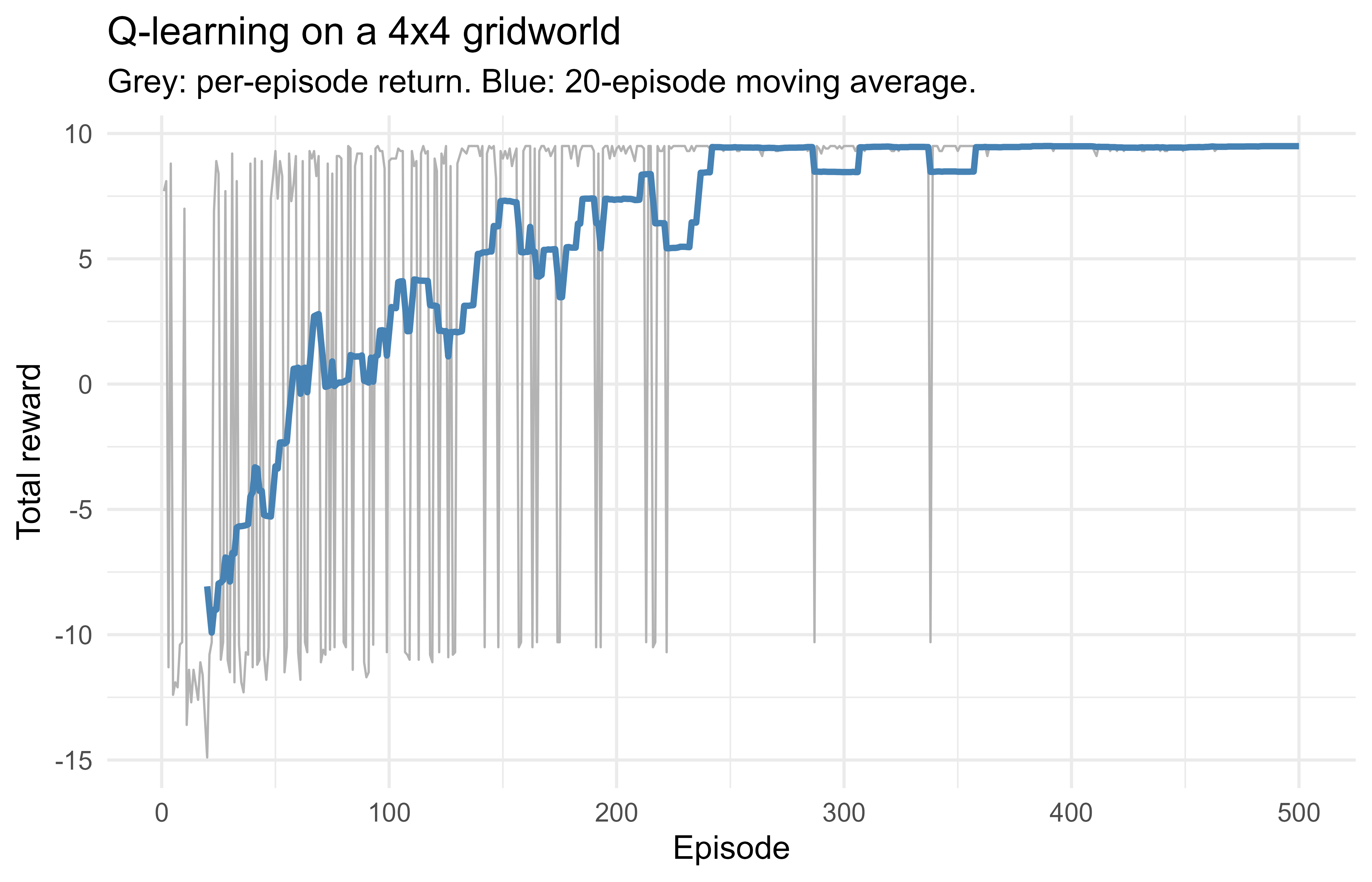
Finally, the learning curve. Plotting return against episode shows the agent improving from random behavior (frequently hitting the trap or wandering) to a stable, near optimal return. A moving average smooths the per episode noise. Figure 71.1 shows this trajectory.
Show code
library(ggplot2)ma<-function(x, k=20L){as.numeric(stats::filter(x, rep(1/k, k), sides =1))}df<-data.frame( episode =seq_along(returns_per_episode), ret =returns_per_episode, smooth =ma(returns_per_episode, 20L))ggplot(df, aes(episode))+geom_line(aes(y =ret), color ="grey70", linewidth =0.4)+geom_line(aes(y =smooth), color ="steelblue", linewidth =1.1, na.rm =TRUE)+labs(x ="Episode", y ="Total reward", title ="Q-learning on a 4x4 gridworld", subtitle ="Grey: per-episode return. Blue: 20-episode moving average.")+theme_minimal(base_size =12)
Figure 71.1: Episode return for tabular Q-learning on the gridworld. The raw return is noisy because of exploration; the moving average shows steady improvement and convergence.
The arrow grid shows the payoff: every cell points along a sensible route toward the goal G, and the cells next to the trap X steer around it rather than into it. The same loop, with the table swapped for a neural network and a replay buffer, is exactly DQN. Keeping the demo tabular makes the convergence visible: the policy arrows and the rising reward curve are the whole story of value based RL on one screen.
Note
The fitted policy reflects the reward you wrote, not your unstated intentions. If you had forgotten the small per step penalty, the agent would have no reason to prefer short paths and might wander indefinitely. This small example already illustrates the single most important lesson in applied RL: the reward function is the specification.
71.8 Computational and sample complexity
The cost of the exact, model-based solvers is easy to state. One sweep of value iteration evaluates Equation 71.3 at every \((s,a)\) pair, each requiring a sum over next states, for \(O(|\mathcal{S}|^2 |\mathcal{A}|)\) work per sweep, and the contraction bound says \(O(\log(1/\epsilon) / \log(1/\gamma))\) sweeps reach error \(\epsilon\). Policy iteration needs far fewer outer iterations (often a handful) but each evaluation step solves a linear system, \(O(|\mathcal{S}|^3)\) if done exactly. The horizon dependence is captured by the effective horizon \(1/(1-\gamma)\): as \(\gamma \to 1\) both the number of sweeps and the variance of sampled returns grow, which is the quantitative reason large \(\gamma\) slows learning.
Sample complexity is the binding constraint in the model-free, deep setting. For tabular Q-learning with a generative model, near-optimal value estimation requires on the order of \(\tilde{O}\big(|\mathcal{S}||\mathcal{A}| / ((1-\gamma)^3 \epsilon^2)\big)\) samples, and the \((1-\gamma)^{-3}\) factor makes long-horizon problems expensive. With function approximation there is no general polynomial guarantee, and the table tradeoff (Table 71.1) reflects this empirically: off-policy value methods reuse each transition many times through the replay buffer and so are more sample-efficient per environment step, whereas on-policy Monte Carlo policy gradients discard data after each update and need more interaction. The deadly triad explains the lack of guarantees: when function approximation, bootstrapping, and off-policy training are combined, the composite update is no longer a contraction in any fixed norm, so the fixed-point argument that underwrites tabular convergence fails and divergence is possible. The DQN devices (replay, target networks, gradient clipping) are heuristics that empirically keep the iteration inside a stable region rather than guarantees that it is a contraction.
71.9 Practical guidance and pitfalls
RL projects fail in characteristic ways, and most of the failures are foreseeable. The following points collect the lessons that save the most time in practice, roughly in the order you will run into them:
Start tabular or small. If your state space is small, a table converges fast and is trivial to debug. Move to function approximation only when you must.
Reward design dominates outcomes. Agents optimize the reward you write, not the one you meant. Sparse rewards make learning hard; dense shaping rewards can introduce unintended shortcuts (reward hacking). Test that the optimal policy under your reward is the behavior you actually want.
Discounting is a modeling choice. A \(\gamma\) too close to \(1\) slows learning and can destabilize bootstrapping; too small makes the agent shortsighted. Tune it.
Exploration must be sufficient and must decay. Too little exploration converges to a suboptimal policy; too much never exploits. Anneal \(\varepsilon\) or temperature.
Deep RL is unstable and sample hungry. The deadly triad (function approximation, bootstrapping, and off policy data together) can cause divergence. Replay buffers, target networks, gradient clipping, and reward or observation normalization exist to fight this. Expect to need many more samples than supervised learning, and seed multiple runs because variance across seeds is large.
Watch for overestimation. The \(\max\) in the Q target biases value estimates upward. Double Q-learning (van Hasselt, 2010; van Hasselt et al., 2016) decouples action selection from evaluation to reduce this.
Evaluate with a separate greedy policy. Training return includes exploration noise. Periodically run the greedy policy with exploration off to measure true progress.
When not to use RL. If you can collect labels and decisions are not sequential, prefer supervised learning. If decisions are one shot with exploration, prefer bandits. RL pays off when delayed, sequential credit assignment is the actual problem.
Tip
Before scaling up, get a tiny version working end to end and confirm the agent solves it. The gridworld in this chapter is a fine starting harness: if a new algorithm cannot beat a 4 by 4 grid, the bug is in the algorithm, not the problem size.
To summarize the chapter in one line: RL formalizes learning from evaluative, delayed feedback as an MDP, value based and policy based methods are two routes to solving it, and the deep variants scale those routes to large inputs at the cost of stability and sample efficiency. The gridworld demo shows the value based route in full, and the same loop with a network in place of the table is the foundation of everything from Atari agents to the alignment of large language models.
71.10 Further reading
Sutton and Barto (2018), Reinforcement Learning: An Introduction (2nd ed.). The standard textbook covering MDPs, TD learning, policy gradients, and exploration.
Watkins and Dayan (1992), Q-learning. The convergence result for tabular Q-learning.
Williams (1992), Simple statistical gradient-following algorithms for connectionist reinforcement learning. The REINFORCE estimator.
Mnih et al. (2015), Human-level control through deep reinforcement learning. The DQN paper introducing replay and target networks.
van Hasselt et al. (2016), Deep reinforcement learning with double Q-learning. Addressing overestimation.
Schulman et al. (2017), Proximal policy optimization algorithms. The PPO objective widely used in actor-critic and RLHF.
Lillicrap et al. (2016), Continuous control with deep reinforcement learning. DDPG for continuous action spaces.
The neural network is doing exactly what it does elsewhere in this book: approximating a function that is too large to write down as a table. In RL the function being approximated is a value or a policy, and the training signal comes from the agent’s own experience rather than a fixed labeled dataset.↩︎
This is a strong assumption, and it is what makes the math tractable. When the raw observation is not Markov (for example, a single video frame does not reveal velocity), practitioners restore the property by stacking recent frames or feeding observations through a recurrent network so the state summarizes enough history.↩︎
This is what separates temporal difference methods from Monte Carlo methods. Monte Carlo waits until the episode ends and uses the actual observed return; TD updates immediately using its own prediction of the future. TD trades a little bias for much lower variance and the ability to learn online, step by step.↩︎
A single Atari screen has \(84 \times 84\) pixels with several intensity levels; the number of distinct states is astronomically larger than any table could hold, and most states are never seen twice. A network instead generalizes across similar states, so experience in one situation improves the estimate for related situations the agent has never encountered.↩︎
Source Code
# Deep Reinforcement Learning {#sec-deep-reinforcement-learning}```{r}#| include: falsesource("_common.R")```Imagine teaching a dog a new trick without ever showing it what to do. You cannot demonstrate the trick and you cannot label each movement as right or wrong. All you can do is hand out treats when the dog happens to do something good. Over many attempts the dog figures out, on its own, what earns treats. Reinforcement learning (RL) is the mathematical version of that story. An agent acts in an environment, receives a numeric reward, and must discover good behavior purely through trial and error.This setting is fundamentally different from supervised learning. In supervised learning a teacher provides the correct answer for every example. In RL the agent is never told the right action; it only sees a scalar reward after acting, and it must work backward from rewards to figure out which actions were worth taking. Deep reinforcement learning (deep RL) is the version of this problem where the value function or the policy is represented by a neural network, which lets the same algorithms scale from small grids to high dimensional inputs such as images or board states.^[The neural network is doing exactly what it does elsewhere in this book: approximating a function that is too large to write down as a table. In RL the function being approximated is a value or a policy, and the training signal comes from the agent's own experience rather than a fixed labeled dataset.]::: {.callout-tip title="Intuition"}Supervised learning answers "what is the label for this input?" Reinforcement learning answers "what should I do now so that things go well later?" The second question is harder because the consequences of an action can show up many steps in the future.:::By the end of this chapter you will understand the core objects of RL (Markov decision processes, value functions, and policies), the two main families of methods (value based and policy based), and the deep learning variants that made RL practical on large problems. The chapter builds intuition first, then the math, then a fully runnable demonstration: a tabular Q-learning agent on a small gridworld implemented in base R, which exposes every moving part without hiding anything inside a library. The chapter builds on the neural network material (@sec-neural-networks) and the contextual bandit chapter (@sec-contextual-bandits), and it sets up the ideas behind techniques such as the alignment of large language models (@sec-llms).## Where reinforcement learning fits in a modern workflowMost production machine learning is supervised: a fixed dataset of inputs and labels, a loss, and a model fit by minimizing that loss. RL applies when the decision you make now changes the data you see next, and when feedback is delayed. Recommendation systems that affect what a user clicks next, inventory and pricing systems, robotics and control, game playing, and the reinforcement learning from human feedback (RLHF) stage used to align large language models are all RL shaped problems.The distinguishing features that should make you reach for RL are:- Sequential decisions, where actions have downstream consequences (credit assignment over time).- Feedback that is evaluative (a reward telling you how good your action was) rather than instructive (a label telling you the right action).- A need to balance exploration (gathering information) against exploitation (using what you already know).If your problem has none of these (you have labels, decisions are one shot, and the data distribution does not depend on your model), supervised learning is simpler, more sample efficient, and easier to debug. A useful middle ground is contextual bandits (@sec-contextual-bandits), which keeps the exploration problem but drops the sequential, multi step structure.::: {.callout-tip title="When to use this"}Reach for RL when the decision you make now changes the data you see next and feedback is delayed. If feedback is immediate and decisions do not affect future inputs, use supervised learning. If decisions are one shot but you still need exploration, use bandits. RL is the right tool only when delayed, sequential credit assignment is genuinely the problem you face.:::## Markov decision processesThe standard formalism is the Markov decision process (MDP), a tuple $(\mathcal{S}, \mathcal{A}, P, R, \gamma)$:- $\mathcal{S}$ is the set of states.- $\mathcal{A}$ is the set of actions.- $P(s' \mid s, a)$ is the transition probability of moving to state $s'$ after taking action $a$ in state $s$.- $R(s, a)$ is the expected immediate reward.- $\gamma \in [0, 1)$ is a discount factor that trades off immediate against future reward.The Markov property says the next state and reward depend only on the current state and action, not on the full history.^[This is a strong assumption, and it is what makes the math tractable. When the raw observation is not Markov (for example, a single video frame does not reveal velocity), practitioners restore the property by stacking recent frames or feeding observations through a recurrent network so the state summarizes enough history.] A policy $\pi(a \mid s)$ is a distribution over actions given a state. Think of the policy as the agent's strategy: given where it is, it tells the agent how to choose what to do. The agent interacts with the environment to produce a trajectory $s_0, a_0, r_0, s_1, a_1, r_1, \dots$, and the quantity it wants to maximize is the expected discounted return$$G_t = \sum_{k=0}^{\infty} \gamma^k\, r_{t+k}.$$The discount $\gamma$ keeps the sum finite and encodes a preference for sooner rewards. With $\gamma$ near $0$ the agent is myopic; with $\gamma$ near $1$ it plans far ahead.::: {.callout-tip title="Intuition"}The discount factor is like compound interest in reverse. A reward received $k$ steps from now is worth only $\gamma^k$ as much as the same reward received right now. A patient agent ($\gamma$ close to $1$) treats distant rewards as nearly as valuable as immediate ones; an impatient agent ($\gamma$ close to $0$) cares almost only about the very next reward.:::### Value functions and the Bellman equationsThe state value function under a policy $\pi$ is the expected return from a state,$$V^\pi(s) = \mathbb{E}_\pi\!\left[ G_t \mid s_t = s \right],$$In words, $V^\pi(s)$ answers "if I start here and follow this strategy, how much total reward should I expect?" The action value (Q) function asks a slightly more specific question: the expected return from taking a particular action $a$ in state $s$ and then following $\pi$,$$Q^\pi(s, a) = \mathbb{E}_\pi\!\left[ G_t \mid s_t = s, a_t = a \right].$$Both satisfy recursive Bellman equations, which follow by splitting the return into the immediate reward plus the discounted return from the next state:$$Q^\pi(s, a) = R(s, a) + \gamma \sum_{s'} P(s' \mid s, a) \sum_{a'} \pi(a' \mid s')\, Q^\pi(s', a').$$The goal is the optimal policy $\pi^*$ whose value dominates every other policy. Its action value $Q^*$ satisfies the Bellman optimality equation, where the inner expectation over the next action is replaced by a maximum:$$Q^*(s, a) = R(s, a) + \gamma \sum_{s'} P(s' \mid s, a) \max_{a'} Q^*(s', a').$$ {#eq-deep-reinforcement-learning-bellman-opt}Once $Q^*$ is known, acting optimally is trivial: pick $\pi^*(s) = \arg\max_a Q^*(s, a)$. This is why so much of RL focuses on estimating $Q^*$.### Deriving the Bellman equations from the returnThe recursion in @eq-deep-reinforcement-learning-bellman-opt is not an assumption; it follows from the definition of the return by linearity of expectation and the Markov property. Write the discounted return as $G_t = r_t + \gamma G_{t+1}$, which is immediate from $G_t = \sum_{k \ge 0} \gamma^k r_{t+k}$. Taking the conditional expectation under $\pi$,$$\begin{aligned}Q^\pi(s,a) &= \mathbb{E}_\pi[\, r_t + \gamma G_{t+1} \mid s_t = s, a_t = a \,] \\&= R(s,a) + \gamma\, \mathbb{E}_\pi[\, G_{t+1} \mid s_t = s, a_t = a \,] \\&= R(s,a) + \gamma \sum_{s'} P(s' \mid s,a)\, \mathbb{E}_\pi[\, G_{t+1} \mid s_{t+1} = s' \,] \\&= R(s,a) + \gamma \sum_{s'} P(s' \mid s,a)\, V^\pi(s'),\end{aligned}$$ {#eq-deep-reinforcement-learning-bellman-derive}where the third line uses the Markov property (conditioning on $(s,a)$ then on $s'$, the future no longer depends on the past) and the fourth uses $V^\pi(s') = \mathbb{E}_\pi[G_{t+1} \mid s_{t+1} = s']$. Substituting $V^\pi(s') = \sum_{a'} \pi(a' \mid s')\, Q^\pi(s',a')$ recovers the action-value Bellman equation stated above. For the optimal value, $V^*(s') = \max_{a'} Q^*(s',a')$, which gives @eq-deep-reinforcement-learning-bellman-opt.### The Bellman operator is a contractionThe reason value iteration and, asymptotically, Q-learning converge is that the Bellman optimality update is a contraction in the supremum norm. Define the Bellman optimality operator $\mathcal{T}$ acting on any action-value table $Q$ by$$(\mathcal{T} Q)(s,a) = R(s,a) + \gamma \sum_{s'} P(s' \mid s,a) \max_{a'} Q(s',a').$$ {#eq-deep-reinforcement-learning-bellman-operator}For any two tables $Q_1, Q_2$, fix a pair $(s,a)$. Using $|\max_{a'} f(a') - \max_{a'} g(a')| \le \max_{a'} |f(a') - g(a')|$,$$\begin{aligned}\big|(\mathcal{T}Q_1)(s,a) - (\mathcal{T}Q_2)(s,a)\big|&= \gamma \left| \sum_{s'} P(s'\mid s,a)\Big( \max_{a'} Q_1(s',a') - \max_{a'} Q_2(s',a') \Big) \right| \\&\le \gamma \sum_{s'} P(s'\mid s,a)\, \big| \max_{a'} Q_1(s',a') - \max_{a'} Q_2(s',a') \big| \\&\le \gamma \sum_{s'} P(s'\mid s,a)\, \max_{a'} \big| Q_1(s',a') - Q_2(s',a') \big| \\&\le \gamma \, \| Q_1 - Q_2 \|_\infty.\end{aligned}$$Taking the supremum over $(s,a)$ on the left gives $\| \mathcal{T}Q_1 - \mathcal{T}Q_2 \|_\infty \le \gamma \, \| Q_1 - Q_2 \|_\infty$. Because $\gamma < 1$, $\mathcal{T}$ is a $\gamma$-contraction, so by the Banach fixed-point theorem it has a unique fixed point, which is $Q^*$, and the iteration $Q_{k+1} = \mathcal{T} Q_k$ converges geometrically: $\| Q_k - Q^* \|_\infty \le \gamma^k \| Q_0 - Q^* \|_\infty$. This is also why $\gamma$ near $1$ slows convergence, since the per-iteration error shrinks only by a factor $\gamma$.::: {.callout-note}The same argument shows the policy-evaluation operator $\mathcal{T}^\pi$ (the version of @eq-deep-reinforcement-learning-bellman-operator with $\max_{a'}$ replaced by $\sum_{a'} \pi(a'\mid s')$) is also a $\gamma$-contraction, with fixed point $V^\pi$. Policy iteration alternates evaluation (solve $V^\pi$) and greedy improvement; each improvement step weakly increases the value at every state (the policy improvement theorem), and since there are finitely many deterministic policies in a finite MDP, it terminates at $\pi^*$ in finitely many iterations.:::We can confirm the geometric contraction rate $\| Q_k - Q^* \|_\infty \le \gamma^k \| Q_0 - Q^* \|_\infty$ numerically on a tiny random MDP using only base R. We build a known model, iterate the Bellman optimality operator to a fixed point $Q^*$, then check that the error contracts by a factor of at most $\gamma$ each step.```{r bellman-contraction-check}set.seed(42)nS <-5L; nA <-3L; gamma <-0.9# Random transition model P[s, a, s'] and reward R[s, a].P <-array(runif(nS * nA * nS), dim =c(nS, nA, nS))for (s in1:nS) for (a in1:nA) P[s, a, ] <- P[s, a, ] /sum(P[s, a, ])R <-matrix(runif(nS * nA), nS, nA)# Bellman optimality operator on a Q-table.bellman_T <-function(Q) { V <-apply(Q, 1, max) # V(s') = max_a Q(s', a) TQ <-matrix(0, nS, nA)for (s in1:nS) for (a in1:nA) TQ[s, a] <- R[s, a] + gamma *sum(P[s, a, ] * V) TQ}# Iterate to the fixed point Q*.Qstar <-matrix(0, nS, nA)for (i in1:500) Qstar <-bellman_T(Qstar)# Track the sup-norm error from an arbitrary start.Q <-matrix(10, nS, nA)errs <-numeric(15)for (k in1:15) { Q <-bellman_T(Q); errs[k] <-max(abs(Q - Qstar)) }ratios <- errs[-1] / errs[-length(errs)] # successive contraction ratioscat("max successive ratio:", round(max(ratios), 4)," (should be <= gamma =", gamma, ")\n")```The largest observed ratio sits at or below $\gamma$, confirming the contraction bound.::: {.callout-important title="Key idea"}The Bellman equation turns a hard global problem (optimize behavior over an entire infinite future) into a local, recursive one (the value of a state equals the immediate reward plus the discounted value of where you land next). Almost every algorithm in this chapter is a way to solve some version of that recursion from sampled experience.:::## Value based methods: Q-learningWhen the transition model $P$ and reward $R$ are known, you can solve the Bellman optimality equation by dynamic programming (value iteration or policy iteration). In most real problems the model is unknown, so the agent must learn from sampled experience. Q-learning is the canonical model free method. It maintains an estimate $Q(s, a)$ and updates it after each transition $(s, a, r, s')$ using the temporal difference (TD) error:$$Q(s, a) \leftarrow Q(s, a) + \alpha \Big[\, r + \gamma \max_{a'} Q(s', a') - Q(s, a) \,\Big],$$ {#eq-deep-reinforcement-learning-qlearn-update}where $\alpha \in (0, 1]$ is the learning rate. The bracketed term is the TD error: the difference between the bootstrapped target $r + \gamma \max_{a'} Q(s', a')$ and the current estimate. "Bootstrapping" here means the update uses the current (imperfect) estimate of the next state's value to improve the estimate of this state, rather than waiting for the true return.^[This is what separates temporal difference methods from Monte Carlo methods. Monte Carlo waits until the episode ends and uses the actual observed return; TD updates immediately using its own prediction of the future. TD trades a little bias for much lower variance and the ability to learn online, step by step.]::: {.callout-tip title="Intuition"}Each Q-learning update nudges the current estimate a fraction $\alpha$ of the way toward a slightly better target. If the target is consistently higher than the current value, the estimate climbs; if lower, it falls. Repeat over enough visits and the estimates settle onto $Q^*$. Q-learning is off policy, meaning it learns about the greedy policy while the data may come from a different (exploratory) behavior policy. Under standard conditions (every state action pair visited infinitely often and a suitably decaying $\alpha$), tabular Q-learning converges to $Q^*$ (Watkins and Dayan, 1992).:::To ensure exploration, a common behavior policy is $\varepsilon$-greedy: with probability $1 - \varepsilon$ take the greedy action $\arg\max_a Q(s, a)$, and with probability $\varepsilon$ take a uniformly random action. Decaying $\varepsilon$ over time shifts the agent from exploring early to exploiting later.### Why Q-learning converges: stochastic approximationThe update @eq-deep-reinforcement-learning-qlearn-update is a stochastic-approximation (Robbins-Monro) scheme for finding the fixed point of the Bellman operator $\mathcal{T}$. To see this, rewrite the update as$$Q_{t+1}(s_t,a_t) = (1 - \alpha_t)\, Q_t(s_t,a_t) + \alpha_t \big[\, r_t + \gamma \max_{a'} Q_t(s_{t+1}, a') \,\big],$$and note that the bracketed sample target is an unbiased estimate of $(\mathcal{T} Q_t)(s_t,a_t)$, because $\mathbb{E}[\, r_t + \gamma \max_{a'} Q_t(s_{t+1},a') \mid s_t,a_t \,] = R(s_t,a_t) + \gamma \sum_{s'} P(s'\mid s_t,a_t) \max_{a'} Q_t(s',a') = (\mathcal{T}Q_t)(s_t,a_t)$. Writing the target as $(\mathcal{T}Q_t)(s_t,a_t)$ plus mean-zero noise, the iteration is the noisy fixed-point search $Q_{t+1} = Q_t + \alpha_t (\mathcal{T}Q_t - Q_t + \text{noise})$. The contraction property of $\mathcal{T}$ supplies the descent direction.The classical convergence theorem (Watkins and Dayan, 1992; Jaakkola, Jordan, and Singh, 1994) states that $Q_t \to Q^*$ with probability one provided:- every state-action pair $(s,a)$ is visited infinitely often (so exploration never stops, which $\varepsilon$-greedy with $\varepsilon > 0$ guarantees), and- the per-pair learning rates satisfy the Robbins-Monro conditions$$\sum_{t} \alpha_t(s,a) = \infty, \qquad \sum_{t} \alpha_t(s,a)^2 < \infty.$$ {#eq-deep-reinforcement-learning-robbins-monro}The first condition forces the steps to be large enough in aggregate to reach $Q^*$ from any start; the second forces them to shrink fast enough that the injected noise averages out. A schedule such as $\alpha_t(s,a) = 1 / (1 + n_t(s,a))$, where $n_t(s,a)$ counts visits, satisfies both. A constant $\alpha$ violates the square-summability condition: the estimates then do not converge to a point but instead hover in a neighborhood of $Q^*$ whose radius scales with $\alpha$, trading asymptotic accuracy for faster tracking. The gridworld demo below uses a constant $\alpha$ for exactly this reason: fast, stable enough on a tiny problem, and the residual noise is invisible at the policy level.::: {.callout-note}The off policy property is what lets $\varepsilon$-greedy work without biasing the result. The agent behaves randomly some of the time to gather information, yet it still learns the value of acting greedily, because the $\max$ in the target always refers to the best action regardless of what action was actually taken.:::### Deep Q-Networks (DQN)Tabular Q-learning stores one number per state action pair, which is impossible when states are images or other high dimensional vectors.^[A single Atari screen has $84 \times 84$ pixels with several intensity levels; the number of distinct states is astronomically larger than any table could hold, and most states are never seen twice. A network instead generalizes across similar states, so experience in one situation improves the estimate for related situations the agent has never encountered.] A Deep Q-Network replaces the table with a neural network $Q(s, a; \theta)$ and fits $\theta$ by minimizing the squared TD error. Naively training this is unstable, so DQN (Mnih et al., 2015) added two ideas that are now standard:1. Experience replay: store transitions $(s, a, r, s')$ in a buffer and train on random minibatches sampled from it. This breaks the temporal correlation between consecutive samples and reuses data.2. A target network: a periodically updated copy $Q(\cdot; \theta^-)$ used to compute the bootstrap target, which stops the target from moving every gradient step.The loss minimized on a minibatch is$$L(\theta) = \mathbb{E}_{(s,a,r,s')}\Big[\big(\, r + \gamma \max_{a'} Q(s', a'; \theta^-) - Q(s, a; \theta) \,\big)^2\Big].$$::: {.callout-warning}Combining a neural network with bootstrapped TD targets is dangerous. Because the same network produces both the prediction and the target, an update can chase a target that it just shifted, sending the values off to infinity. Experience replay and the target network exist precisely to tame this feedback loop.:::The following sketch shows the structure of a DQN training step in keras. It is kept `eval=FALSE` because it is meant as a reference, not a runnable demo: a full agent also needs an environment loop, and the keras backend is not assumed available in this build.```{r dqn-keras-sketch, eval=FALSE}library(keras)# Q-network: maps a state vector to one Q-value per action.build_q_network <-function(state_dim, n_actions) {keras_model_sequential() |>layer_dense(units =64, activation ="relu",input_shape = state_dim) |>layer_dense(units =64, activation ="relu") |>layer_dense(units = n_actions, activation ="linear")}online_net <-build_q_network(state_dim =4, n_actions =2)target_net <-build_q_network(state_dim =4, n_actions =2)target_net |>set_weights(get_weights(online_net))online_net |>compile(optimizer =optimizer_adam(1e-3), loss ="mse")# One gradient step on a minibatch drawn from the replay buffer.dqn_train_step <-function(batch, gamma =0.99) {# batch: list with states, actions, rewards, next_states, done q_next <-predict(target_net, batch$next_states, verbose =0) max_next <-apply(q_next, 1, max) targets_for_taken <- batch$rewards + gamma * max_next * (1- batch$done) q_now <-predict(online_net, batch$states, verbose =0) idx <-cbind(seq_len(nrow(q_now)), batch$actions +1L) # actions 0-indexed q_now[idx] <- targets_for_taken # only the taken action gets a new target online_net |>fit(batch$states, q_now, epochs =1, verbose =0)}# Periodically: target_net |> set_weights(get_weights(online_net))```### Maximization bias and Double Q-learningThe $\max$ in the Q target systematically overestimates. The issue is that $\mathbb{E}[\max_a \hat{Q}(s',a)] \ge \max_a \mathbb{E}[\hat{Q}(s',a)]$ by Jensen's inequality, since the maximum is convex. When the $\hat{Q}(s',a)$ are noisy estimates of equal true values, the same noisy sample is used both to pick the maximizing action and to read off its value, so positive errors are selectively propagated into the target and the bias compounds through bootstrapping. As a concrete case, if $\hat{Q}(s',a) = \mu + \epsilon_a$ with i.i.d. mean-zero noise of variance $\sigma^2$ across $m$ actions whose true values are all $\mu$, then $\mathbb{E}[\max_a \hat{Q}(s',a)] = \mu + \mathbb{E}[\max_a \epsilon_a] > \mu$, and for Gaussian noise the bias grows like $\sigma \sqrt{2 \log m}$, increasing with the number of actions.Double Q-learning (van Hasselt, 2010) removes this by decoupling selection from evaluation. Maintain two estimators $Q^A, Q^B$. To update $Q^A$, select the greedy action with $Q^A$ but evaluate it with $Q^B$:$$Q^A(s,a) \leftarrow Q^A(s,a) + \alpha \Big[\, r + \gamma\, Q^B\big(s', \arg\max_{a'} Q^A(s',a')\big) - Q^A(s,a) \,\Big],$$ {#eq-deep-reinforcement-learning-double-q}and symmetrically for $Q^B$ (choosing which to update at random each step). Because the noise in the selector $Q^A$ is independent of the noise in the evaluator $Q^B$, the selected action's value is no longer biased upward in expectation. Double DQN (van Hasselt et al., 2016) applies the same idea cheaply in the deep setting by reusing the online network for selection and the target network for evaluation, replacing the DQN target with $r + \gamma\, Q(s', \arg\max_{a'} Q(s',a'; \theta); \theta^-)$.## Policy based methodsSo far the agent has learned a value and then read off a policy by taking the action with the highest value. There is a more direct route. Policy based methods skip the value table and parameterize the policy itself as $\pi_\theta(a \mid s)$, then optimize the expected return $J(\theta) = \mathbb{E}_{\pi_\theta}[G_0]$ by gradient ascent. This is attractive when the action space is continuous or very large (where taking a $\max$ over actions is awkward or impossible), and when a stochastic policy is genuinely desirable, for example in games where being predictable is a weakness.::: {.callout-important title="Key idea"}Value based methods learn "how good is each action?" and act greedily. Policy based methods learn "what should I do?" directly and adjust that mapping to earn more reward. The two views are complementary, and actor-critic methods, below, combine them.:::### The policy gradient and REINFORCEThe policy gradient theorem gives an expression for $\nabla_\theta J$ that does not require differentiating through the environment dynamics:$$\nabla_\theta J(\theta) = \mathbb{E}_{\pi_\theta}\!\left[ \sum_{t \ge 0} \gamma^t\, \nabla_\theta \log \pi_\theta(a_t \mid s_t)\, G_t \right].$$ {#eq-deep-reinforcement-learning-pg}#### Deriving the policy gradientThe trajectory form is the cleanest derivation. Let $\tau = (s_0, a_0, s_1, a_1, \dots)$ be a trajectory, $R(\tau) = \sum_{t} \gamma^t r_t$ its return, and$$p_\theta(\tau) = \rho_0(s_0) \prod_{t \ge 0} \pi_\theta(a_t \mid s_t)\, P(s_{t+1} \mid s_t, a_t)$$its probability under policy $\pi_\theta$, where $\rho_0$ is the initial-state distribution. The objective is $J(\theta) = \mathbb{E}_{\tau \sim p_\theta}[R(\tau)] = \int p_\theta(\tau) R(\tau)\, d\tau$. Differentiating and applying the log-derivative identity $\nabla_\theta p_\theta = p_\theta \nabla_\theta \log p_\theta$,$$\nabla_\theta J(\theta) = \int \nabla_\theta p_\theta(\tau)\, R(\tau)\, d\tau= \int p_\theta(\tau)\, \nabla_\theta \log p_\theta(\tau)\, R(\tau)\, d\tau= \mathbb{E}_{\tau}\!\left[ \nabla_\theta \log p_\theta(\tau)\, R(\tau) \right].$$The key simplification is that in $\log p_\theta(\tau)$ only the policy factors depend on $\theta$; the dynamics $P$ and the initial distribution $\rho_0$ drop out under the gradient:$$\nabla_\theta \log p_\theta(\tau) = \nabla_\theta \Big[ \log \rho_0(s_0) + \sum_t \log \pi_\theta(a_t \mid s_t) + \sum_t \log P(s_{t+1}\mid s_t,a_t) \Big] = \sum_t \nabla_\theta \log \pi_\theta(a_t \mid s_t).$$This is why policy gradients are model-free: the gradient never references $P$. Substituting gives $\nabla_\theta J = \mathbb{E}_\tau\big[ (\sum_t \nabla_\theta \log \pi_\theta(a_t\mid s_t))\, R(\tau) \big]$. A further refinement uses causality: an action $a_t$ cannot influence rewards earned before time $t$, so each $\nabla_\theta \log \pi_\theta(a_t \mid s_t)$ may be multiplied by only the discounted return from $t$ onward, which is $\gamma^t G_t$, rather than the full $R(\tau)$. The discarded cross-terms have expectation zero, leaving @eq-deep-reinforcement-learning-pg. (Practical REINFORCE often drops the $\gamma^t$ weighting, which biases the gradient but works well in practice.)The intuition is the log likelihood trick: increase the log probability of actions that led to high return and decrease it for actions that led to low return, weighted by how good the return was. It is reinforcement in the literal sense, make the good actions more likely next time. REINFORCE (Williams, 1992) is the Monte Carlo estimate of this gradient. It runs full episodes, computes the realized return $G_t$ from each step, and takes an ascent step. The estimator is unbiased but high variance, so a state dependent baseline $b(s_t)$ is subtracted (it does not change the expectation):$$\nabla_\theta J(\theta) = \mathbb{E}_{\pi_\theta}\!\left[ \sum_{t \ge 0} \gamma^t\, \nabla_\theta \log \pi_\theta(a_t \mid s_t)\, \big(G_t - b(s_t)\big) \right].$$ {#eq-deep-reinforcement-learning-pg-baseline}#### Why the baseline is unbiased, and why it helpsSubtracting any baseline $b(s_t)$ that does not depend on the action leaves the gradient unchanged in expectation. The added term vanishes because the score function integrates to zero. Conditioning on $s_t$,$$\mathbb{E}_{a_t \sim \pi_\theta(\cdot \mid s_t)}\!\big[ \nabla_\theta \log \pi_\theta(a_t \mid s_t)\, b(s_t) \big]= b(s_t) \sum_{a} \pi_\theta(a \mid s_t)\, \nabla_\theta \log \pi_\theta(a \mid s_t)= b(s_t)\, \nabla_\theta \sum_a \pi_\theta(a \mid s_t) = b(s_t)\, \nabla_\theta 1 = 0.$$ {#eq-deep-reinforcement-learning-baseline-zero}So @eq-deep-reinforcement-learning-pg-baseline is an unbiased estimator for any state-dependent $b$. Its value is variance reduction. For a scalar parameter, the per-step contribution is $g(a) = \nabla_\theta \log \pi_\theta(a\mid s)\,(G - b)$, whose variance is $\mathrm{Var}(g) = \mathbb{E}[(\nabla_\theta\log\pi_\theta)^2 (G-b)^2] - (\nabla_\theta J)^2$. Minimizing over $b$ by setting $\partial \mathrm{Var}/\partial b = 0$ gives the variance-optimal baseline$$b^\star = \frac{\mathbb{E}\big[(\nabla_\theta \log \pi_\theta)^2\, G\big]}{\mathbb{E}\big[(\nabla_\theta \log \pi_\theta)^2\big]},$$ {#eq-deep-reinforcement-learning-optimal-baseline}a gradient-magnitude-weighted average return. In practice the simpler choice $b(s) = V^\pi(s)$ captures most of the benefit: it centers $G_t$ on its conditional mean so the weight $G_t - V(s_t)$ becomes the advantage, which is small whenever the action was merely average and large only when it genuinely beat or missed expectations. This is the formal reason actor-critic methods reduce variance, and it motivates using a learned $V_w$ as the baseline.### Actor-critic methodsActor-critic methods keep an actor (the policy $\pi_\theta$) and a critic (a value estimate $V_w$ or $Q_w$). The critic supplies a low variance learning signal to the actor, typically the advantage$$A(s_t, a_t) = Q(s_t, a_t) - V(s_t) \approx r_t + \gamma V_w(s_{t+1}) - V_w(s_t),$$which measures how much better action $a_t$ was than the policy's average behavior in state $s_t$. A positive advantage means "that action beat expectations, do more of it"; a negative advantage means the opposite. The actor update becomes $\nabla_\theta \log \pi_\theta(a_t \mid s_t)\, A(s_t, a_t)$ and the critic is fit to reduce its own TD error.The one-step advantage $\delta_t = r_t + \gamma V_w(s_{t+1}) - V_w(s_t)$ has low variance but is biased whenever $V_w \ne V^\pi$. The opposite extreme, the Monte Carlo advantage $G_t - V_w(s_t)$, is nearly unbiased but high variance. Generalized advantage estimation (GAE; Schulman et al., 2016) interpolates between them with a parameter $\lambda \in [0,1]$ by taking an exponentially weighted sum of the TD residuals:$$\hat{A}_t^{\text{GAE}(\gamma,\lambda)} = \sum_{l \ge 0} (\gamma \lambda)^l\, \delta_{t+l}, \qquad \delta_t = r_t + \gamma V_w(s_{t+1}) - V_w(s_t).$$ {#eq-deep-reinforcement-learning-gae}Setting $\lambda = 0$ recovers the one-step advantage $\delta_t$ (low variance, biased); $\lambda = 1$ telescopes to $\sum_{l\ge0}\gamma^l r_{t+l} - V_w(s_t) = G_t - V_w(s_t)$ (the Monte Carlo advantage, unbiased, high variance). Intermediate $\lambda$, typically $0.9$ to $0.97$, trades the two off and is one of the most important knobs in modern policy-gradient implementations.::: {.callout-tip title="Intuition"}Think of the actor as a student trying actions and the critic as a coach. The coach does not dictate moves; it just says "that was better than I expected" or "worse than I expected," and the student adjusts. Because the coach's running expectation absorbs most of the variability, the feedback is far less noisy than raw returns. Modern algorithms in this family (A2C, PPO, SAC) add tricks to stay stable, such as clipping the size of each policy update (PPO, Schulman et al., 2017). PPO in particular is the workhorse behind the RLHF stage of instruction tuned language models.:::#### The PPO clipped objectiveVanilla policy gradient takes one update per batch of fresh on-policy data, which is sample-inefficient. We would like to reuse a batch for several gradient steps, but after the policy moves the data is no longer on-policy. Importance sampling corrects for this: with $r_t(\theta) = \pi_\theta(a_t\mid s_t) / \pi_{\theta_{\text{old}}}(a_t \mid s_t)$ the ratio between the current and data-collecting policies, the surrogate objective $\mathbb{E}[\, r_t(\theta)\, \hat{A}_t \,]$ has the same gradient at $\theta = \theta_{\text{old}}$ as the policy gradient. The danger is that maximizing it freely lets $r_t$ blow up, taking a destructively large step. PPO (Schulman et al., 2017) bounds the step by clipping the ratio:$$L^{\text{CLIP}}(\theta) = \mathbb{E}_t\Big[ \min\big( r_t(\theta)\, \hat{A}_t,\; \operatorname{clip}(r_t(\theta), 1-\epsilon, 1+\epsilon)\, \hat{A}_t \big) \Big].$$ {#eq-deep-reinforcement-learning-ppo}The $\min$ with the clipped term makes the objective a pessimistic (lower) bound on the unclipped surrogate. When $\hat{A}_t > 0$, the objective stops rewarding increases in $r_t$ beyond $1 + \epsilon$; when $\hat{A}_t < 0$, it stops past $1 - \epsilon$. Either way the incentive to move the policy far from $\theta_{\text{old}}$ in a single batch is removed, which approximates the trust-region constraint of TRPO without a second-order solve. Typical $\epsilon$ is $0.1$ to $0.2$. This clipped surrogate, combined with a value-function loss and an entropy bonus, is the full PPO loss used in RLHF.## Comparing the method families@tbl-deep-reinforcement-learning-method-families summarizes how the main approaches differ and when each is a reasonable default.| Property | Value based (Q-learning, DQN) | Policy gradient (REINFORCE) | Actor-critic (A2C, PPO, SAC) ||---|---|---|---|| What is learned | Action value $Q(s,a)$ | Policy $\pi_\theta(a\mid s)$ | Policy plus value critic || Action spaces | Discrete | Discrete or continuous | Discrete or continuous || On vs off policy | Off policy | On policy | Either, depending on variant || Sample efficiency | Higher (replay reuses data) | Lower (Monte Carlo returns) | Medium to high || Gradient variance | Not applicable | High | Reduced by the critic || Stochastic policy | Indirect (via $\varepsilon$-greedy) | Native | Native || Typical failure mode | Overestimation, instability | High variance, slow | Critic bias, tuning sensitivity || Good default for | Discrete control, pixels | Simple continuous tasks, teaching | Most large scale problems |: Comparison of the three main reinforcement learning method families across what they learn, the action spaces they handle, sample efficiency, and typical failure modes. {#tbl-deep-reinforcement-learning-method-families}## Exploration strategiesExploration is the part of RL with no supervised analog. A greedy agent that always exploits its current estimates can lock onto a suboptimal action before it has tried the better one, a problem with no equivalent in supervised learning, where the dataset is fixed and never depends on the model's choices.::: {.callout-warning}The exploration versus exploitation tradeoff is unavoidable. Too little exploration and the agent commits early to a mediocre policy; too much and it keeps gambling on random actions instead of using what it has learned. Almost every exploration method below is a different way to schedule the shift from the first regime to the second.:::Several standard strategies manage this tradeoff:- $\varepsilon$-greedy: random action with probability $\varepsilon$, otherwise greedy. Simple and widely used; decay $\varepsilon$ over time.- Boltzmann (softmax) exploration: sample actions with probability $\propto \exp(Q(s,a)/\tau)$, where temperature $\tau$ controls randomness.- Optimistic initialization: start $Q$ values high so unvisited actions look attractive and get tried.- Upper confidence bound (UCB) and Thompson sampling: pick actions by an optimistic or posterior sampled estimate, which is the dominant idea in bandits (@sec-multi-armed-bandits) and carries over to RL.- Intrinsic motivation: add a bonus for visiting novel states, useful when external reward is sparse.## Runnable demo: tabular Q-learning on a gridworldThe cleanest way to internalize Q-learning is to watch it solve a small gridworld with nothing but base R. The environment is a 4 by 4 grid. The agent starts in the top left, the goal is the bottom right, and one cell is a trap. Each step gives a small negative reward (to encourage short paths), reaching the goal gives a large positive reward, and the trap gives a large negative reward. The agent can move up, down, left, or right; moves into a wall leave it in place.::: {.callout-tip}Read the next four chunks as one story. The first defines the environment (geometry, transitions, rewards), the second is the learning loop, the third reads the learned policy off the table, and the fourth plots the learning curve. Everything is plain base R plus `ggplot2`, so you can step through it line by line and inspect the `Q` matrix at any point.:::```{r grid-setup}.libPaths(c("C:/Users/miken/R/library-4.4", .libPaths()))set.seed(1)# Grid geometry: 4x4, states numbered 1..16 row-major.n_rows <-4Ln_cols <-4Ln_states <- n_rows * n_colsactions <-c("up", "down", "left", "right")n_actions <-length(actions)start_state <-1L # top-leftgoal_state <- n_states # bottom-right (16)trap_state <-11L # one penalty cell# Convert between linear index and (row, col).to_rc <-function(s) c(row = ((s -1L) %/% n_cols) +1L,col = ((s -1L) %% n_cols) +1L)to_state <-function(r, c) (r -1L) * n_cols + c# Deterministic transition: returns the next state for a (state, action).step_state <-function(s, a) { rc <-to_rc(s); r <- rc["row"]; c <- rc["col"]if (a =="up") r <-max(1L, r -1L)if (a =="down") r <-min(n_rows, r +1L)if (a =="left") c <-max(1L, c -1L)if (a =="right") c <-min(n_cols, c +1L)as.integer(to_state(r, c))}# Reward and termination for landing in a state.reward_of <-function(s) {if (s == goal_state) return(10)if (s == trap_state) return(-10)-0.1# step cost}is_terminal <-function(s) s == goal_state || s == trap_state```With the environment defined, the Q-learning loop is short. The agent runs many episodes; in each it acts $\varepsilon$-greedily, applies the TD update, and decays $\varepsilon$.```{r q-learning-train}gamma <-0.95# discountalpha <-0.5# learning raten_episodes <-500Lmax_steps <-100Leps_start <-1.0eps_end <-0.05eps_decay <-0.99# Q-table: rows are states, columns are actions.Q <-matrix(0, nrow = n_states, ncol = n_actions,dimnames =list(NULL, actions))epsilon <- eps_startreturns_per_episode <-numeric(n_episodes)for (ep inseq_len(n_episodes)) { s <- start_state total_reward <-0for (t inseq_len(max_steps)) {# epsilon-greedy action choiceif (runif(1) < epsilon) { a_idx <-sample.int(n_actions, 1L) } else { a_idx <-which.max(Q[s, ]) # ties: first max } a <- actions[a_idx] s_next <-step_state(s, a) r <-reward_of(s_next) total_reward <- total_reward + r# Q-learning TD update best_next <-if (is_terminal(s_next)) 0elsemax(Q[s_next, ]) td_target <- r + gamma * best_next Q[s, a_idx] <- Q[s, a_idx] + alpha * (td_target - Q[s, a_idx]) s <- s_nextif (is_terminal(s)) break } returns_per_episode[ep] <- total_reward epsilon <-max(eps_end, epsilon * eps_decay)}cat("Final epsilon:", round(epsilon, 3), "\n")```The learned greedy policy is read directly off the Q-table. The next chunk prints it as an arrow grid so you can see the agent routing toward the goal and around the trap.```{r show-policy}arrow_of <-c(up ="^", down ="v", left ="<", right =">")policy_grid <-matrix("", nrow = n_rows, ncol = n_cols)for (s inseq_len(n_states)) { rc <-to_rc(s)if (s == goal_state) { policy_grid[rc["row"], rc["col"]] <-"G" } elseif (s == trap_state) { policy_grid[rc["row"], rc["col"]] <-"X" } else { best_a <- actions[which.max(Q[s, ])] policy_grid[rc["row"], rc["col"]] <- arrow_of[best_a] }}cat("Learned greedy policy (S=start, G=goal, X=trap):\n\n")policy_grid[to_rc(start_state)["row"], to_rc(start_state)["col"]] <-"S"for (r inseq_len(n_rows)) {cat(" ", paste(policy_grid[r, ], collapse =" "), "\n")}```Finally, the learning curve. Plotting return against episode shows the agent improving from random behavior (frequently hitting the trap or wandering) to a stable, near optimal return. A moving average smooths the per episode noise. @fig-deep-reinforcement-learning-reward-curve shows this trajectory.```{r fig-deep-reinforcement-learning-reward-curve, fig.cap="Episode return for tabular Q-learning on the gridworld. The raw return is noisy because of exploration; the moving average shows steady improvement and convergence.", fig.width=7, fig.height=4.5}library(ggplot2)ma <-function(x, k =20L) {as.numeric(stats::filter(x, rep(1/ k, k), sides =1))}df <-data.frame(episode =seq_along(returns_per_episode),ret = returns_per_episode,smooth =ma(returns_per_episode, 20L))ggplot(df, aes(episode)) +geom_line(aes(y = ret), color ="grey70", linewidth =0.4) +geom_line(aes(y = smooth), color ="steelblue", linewidth =1.1,na.rm =TRUE) +labs(x ="Episode", y ="Total reward",title ="Q-learning on a 4x4 gridworld",subtitle ="Grey: per-episode return. Blue: 20-episode moving average.") +theme_minimal(base_size =12)```The arrow grid shows the payoff: every cell points along a sensible route toward the goal `G`, and the cells next to the trap `X` steer around it rather than into it. The same loop, with the table swapped for a neural network and a replay buffer, is exactly DQN. Keeping the demo tabular makes the convergence visible: the policy arrows and the rising reward curve are the whole story of value based RL on one screen.::: {.callout-note}The fitted policy reflects the reward you wrote, not your unstated intentions. If you had forgotten the small per step penalty, the agent would have no reason to prefer short paths and might wander indefinitely. This small example already illustrates the single most important lesson in applied RL: the reward function is the specification.:::## Computational and sample complexityThe cost of the exact, model-based solvers is easy to state. One sweep of value iteration evaluates @eq-deep-reinforcement-learning-bellman-operator at every $(s,a)$ pair, each requiring a sum over next states, for $O(|\mathcal{S}|^2 |\mathcal{A}|)$ work per sweep, and the contraction bound says $O(\log(1/\epsilon) / \log(1/\gamma))$ sweeps reach error $\epsilon$. Policy iteration needs far fewer outer iterations (often a handful) but each evaluation step solves a linear system, $O(|\mathcal{S}|^3)$ if done exactly. The horizon dependence is captured by the effective horizon $1/(1-\gamma)$: as $\gamma \to 1$ both the number of sweeps and the variance of sampled returns grow, which is the quantitative reason large $\gamma$ slows learning.Sample complexity is the binding constraint in the model-free, deep setting. For tabular Q-learning with a generative model, near-optimal value estimation requires on the order of $\tilde{O}\big(|\mathcal{S}||\mathcal{A}| / ((1-\gamma)^3 \epsilon^2)\big)$ samples, and the $(1-\gamma)^{-3}$ factor makes long-horizon problems expensive. With function approximation there is no general polynomial guarantee, and the table tradeoff (@tbl-deep-reinforcement-learning-method-families) reflects this empirically: off-policy value methods reuse each transition many times through the replay buffer and so are more sample-efficient per environment step, whereas on-policy Monte Carlo policy gradients discard data after each update and need more interaction. The deadly triad explains the lack of guarantees: when function approximation, bootstrapping, and off-policy training are combined, the composite update is no longer a contraction in any fixed norm, so the fixed-point argument that underwrites tabular convergence fails and divergence is possible. The DQN devices (replay, target networks, gradient clipping) are heuristics that empirically keep the iteration inside a stable region rather than guarantees that it is a contraction.## Practical guidance and pitfallsRL projects fail in characteristic ways, and most of the failures are foreseeable. The following points collect the lessons that save the most time in practice, roughly in the order you will run into them:- Start tabular or small. If your state space is small, a table converges fast and is trivial to debug. Move to function approximation only when you must.- Reward design dominates outcomes. Agents optimize the reward you write, not the one you meant. Sparse rewards make learning hard; dense shaping rewards can introduce unintended shortcuts (reward hacking). Test that the optimal policy under your reward is the behavior you actually want.- Discounting is a modeling choice. A $\gamma$ too close to $1$ slows learning and can destabilize bootstrapping; too small makes the agent shortsighted. Tune it.- Exploration must be sufficient and must decay. Too little exploration converges to a suboptimal policy; too much never exploits. Anneal $\varepsilon$ or temperature.- Deep RL is unstable and sample hungry. The deadly triad (function approximation, bootstrapping, and off policy data together) can cause divergence. Replay buffers, target networks, gradient clipping, and reward or observation normalization exist to fight this. Expect to need many more samples than supervised learning, and seed multiple runs because variance across seeds is large.- Watch for overestimation. The $\max$ in the Q target biases value estimates upward. Double Q-learning (van Hasselt, 2010; van Hasselt et al., 2016) decouples action selection from evaluation to reduce this.- Evaluate with a separate greedy policy. Training return includes exploration noise. Periodically run the greedy policy with exploration off to measure true progress.- When not to use RL. If you can collect labels and decisions are not sequential, prefer supervised learning. If decisions are one shot with exploration, prefer bandits. RL pays off when delayed, sequential credit assignment is the actual problem.::: {.callout-tip}Before scaling up, get a tiny version working end to end and confirm the agent solves it. The gridworld in this chapter is a fine starting harness: if a new algorithm cannot beat a 4 by 4 grid, the bug is in the algorithm, not the problem size.:::To summarize the chapter in one line: RL formalizes learning from evaluative, delayed feedback as an MDP, value based and policy based methods are two routes to solving it, and the deep variants scale those routes to large inputs at the cost of stability and sample efficiency. The gridworld demo shows the value based route in full, and the same loop with a network in place of the table is the foundation of everything from Atari agents to the alignment of large language models.## Further reading- Sutton and Barto (2018), Reinforcement Learning: An Introduction (2nd ed.). The standard textbook covering MDPs, TD learning, policy gradients, and exploration.- Watkins and Dayan (1992), Q-learning. The convergence result for tabular Q-learning.- Williams (1992), Simple statistical gradient-following algorithms for connectionist reinforcement learning. The REINFORCE estimator.- Mnih et al. (2015), Human-level control through deep reinforcement learning. The DQN paper introducing replay and target networks.- van Hasselt et al. (2016), Deep reinforcement learning with double Q-learning. Addressing overestimation.- Schulman et al. (2017), Proximal policy optimization algorithms. The PPO objective widely used in actor-critic and RLHF.- Lillicrap et al. (2016), Continuous control with deep reinforcement learning. DDPG for continuous action spaces.