Imagine you had to describe a friend’s face over the phone so that a sketch artist on the other end could draw it. You would not read off the color of every pixel. You would say a few things that matter: round face, dark curly hair, glasses, a small scar above the left eyebrow. From that short description the artist can reconstruct something close to the original. You have just done by hand what an autoencoder does automatically: compress a high-dimensional thing into a short summary, then rebuild it from that summary.
An autoencoder is a neural network trained to copy its input to its output. That sounds pointless, because copying is trivial. The trick is that the network is forced to pass the data through a low-capacity intermediate representation, so the copying cannot be perfect. To reconstruct the input well despite that constraint, the network must learn what is worth keeping. What it learns to keep in that intermediate representation is a compressed code for the data. This makes the autoencoder a tool for representation learning, where the goal is to discover useful features without labels.1
Key idea
An autoencoder is not interesting because it can reconstruct the input. It is interesting because of what it is forced to throw away to do so. The discarded information is noise and redundancy; the retained information is the structure of the data.
By the end of this chapter you will understand the encoder, the decoder, and the bottleneck that makes the whole thing work; you will see the precise sense in which a linear autoencoder is just PCA in disguise; you will meet the main regularized variants (denoising, sparse, contractive) and the variational autoencoder used for generation; and you will run a small demonstration in base R that confirms the linear-autoencoder-equals-PCA result numerically. Autoencoders sit next to the dimension reduction chapter (Chapter 27) as the nonlinear generalization of the ideas you saw there.
41.1 Encoder, Decoder, and the Bottleneck
Every autoencoder is built from two halves that work in opposite directions. The first half squeezes the data down into a short code; the second half tries to rebuild the original from that code. Training rewards the network when the rebuilt output matches the input.
An autoencoder has two parts. The encoder maps an input \(x \in \mathbb{R}^p\) to a code \(z \in \mathbb{R}^k\),
\[
z = f_\theta(x),
\]
and the decoder maps the code back to the input space,
\[
\hat{x} = g_\phi(z).
\]
Training minimizes a reconstruction loss over the data. With squared error the objective is
In words, we want the round trip from input to code and back to land as close to the original input as possible, averaged over the data.2
Everything then hinges on one number: the dimension \(k\) of the code. It controls how much room the network has to store information, and therefore what it can and cannot do. There are two regimes to distinguish.
An undercomplete autoencoder has \(k < p\). The code is smaller than the input, so the network cannot copy every input perfectly. It must use the limited capacity of the code to capture the structure that matters most for reconstruction. The layer that holds \(z\) is called the bottleneck.
An overcomplete autoencoder has \(k \ge p\). Here the code is at least as large as the input, and the network can learn the identity map and reconstruct everything with zero error. That solution is useless because it stores the data rather than a representation of it. Overcomplete autoencoders are only interesting when some form of regularization is added to stop the trivial copy.
The bottleneck is the mechanism that turns a copy machine into a feature learner. By restricting how much information can flow from input to output, it forces the encoder to throw away noise and redundancy and keep the directions that explain the data.
Intuition
Think of the bottleneck as a narrow doorway. If you must pass all your belongings through a doorway only \(k\) items wide, you will carry the essentials and leave the clutter behind. The width \(k\) decides how much detail survives the trip.
Warning
An overcomplete autoencoder with no regularization will happily learn to do nothing useful, achieving zero reconstruction error by memorizing the identity. If you widen the code to \(k \ge p\), you must add one of the constraints from the Regularized Autoencoders section, or the model learns nothing about the data.
41.2 Linear Autoencoders Recover the Principal Subspace
Before reaching for nonlinear networks, it pays to ask what the simplest possible autoencoder learns. The answer is reassuring and clarifying: a linear autoencoder learns exactly the same thing as Principal Component Analysis. This is worth establishing carefully, because it tells us where the power of autoencoders actually comes from (the answer, given at the end of this section, is nonlinearity).
The simplest autoencoder uses linear encoder and decoder with no nonlinear activations,
\[
z = W x, \qquad \hat{x} = U z = U W x,
\]
where \(W\) is \(k \times p\) and \(U\) is \(p \times k\). Assume the data are centered so that \(\frac{1}{n}\sum_i x_i = 0\). The training objective is
\[
\min_{U, W} \; \sum_{i=1}^n \lVert x_i - U W x_i \rVert^2 .
\]
The key theoretical result, due to Baldi and Hornik (1989), is that the global minimum of this loss is reached when \(U W\) equals the orthogonal projection onto the subspace spanned by the top \(k\) principal components of the data. In other words, a linear autoencoder with squared-error loss learns the same subspace that PCA finds.
Key idea
A linear autoencoder is PCA wearing a neural-network costume. Training it by gradient descent and computing the top principal components are two routes to the same low-dimensional subspace.
The reasoning is direct. The composed map \(M = UW\) has rank at most \(k\), so the problem is to find the rank-\(k\) matrix \(M\) that best reconstructs the centered data in squared error,
Let \(X\) be the \(n \times p\) matrix with the centered observations in its rows and let \(\Sigma = \frac{1}{n} X^\top X\) be the sample covariance. The minimizing \(M\) is the projection \(M = V_k V_k^\top\), where \(V_k\) holds the top \(k\) eigenvectors of \(\Sigma\), equivalently the top \(k\) right singular vectors of \(X\). This is the Eckart and Young low-rank approximation result, and it is exactly the rank-\(k\) representation that PCA produces. See the dimension reduction chapter (Chapter 27) for the PCA derivation through the singular value decomposition.
41.2.0.1 Deriving the optimal reconstruction
It is worth carrying the algebra through, because the derivation pins down both the optimal map and the residual error in closed form. Stacking the residuals into the matrix \(X - XM^\top\) (each row is \(x_i^\top - x_i^\top M^\top\)), the objective is the squared Frobenius norm
\[
\sum_{i=1}^n \lVert x_i - M x_i \rVert^2 = \lVert X - X M^\top \rVert_F^2 .
\]
When \(M = M^\top = P\) is a rank-\(k\) orthogonal projector this is \(\lVert X - XP \rVert_F^2 = \lVert X(I - P) \rVert_F^2\). Write the SVD \(X = U_X D V^\top\) with singular values \(d_1 \ge d_2 \ge \cdots \ge d_p \ge 0\). The Eckart and Young theorem states that among all matrices of rank at most \(k\), the best Frobenius approximation of \(X\) is its truncated SVD \(X_k = U_X D_k V^\top\) obtained by zeroing all but the top \(k\) singular values, and the residual is
\[
\min_{\operatorname{rank}(\hat X)\le k} \lVert X - \hat X \rVert_F^2 = \sum_{j=k+1}^{p} d_j^2 .
\tag{41.1}\]
Any reconstruction of the form \(XM^\top\) with \(\operatorname{rank}(M)\le k\) has rank at most \(k\), so it cannot beat the truncated SVD. The truncation is itself achieved by an orthogonal projector, since \(X_k = X V_k V_k^\top\), so setting \(M = V_k V_k^\top\) attains the bound. Dividing by \(n\), the per-observation reconstruction error at the optimum is \(\frac{1}{n}\sum_{j=k+1}^{p} d_j^2 = \sum_{j=k+1}^{p}\lambda_j\), the sum of the discarded eigenvalues \(\lambda_j\) of \(\Sigma\). This is precisely the closed form the demonstration below checks numerically.
A short calculation explains why the projector form is optimal among symmetric candidates and clarifies the link to maximizing variance. For an orthogonal projector \(P = V_k V_k^\top\),
using \(P^2 = P = P^\top\). Since \(\operatorname{tr}(X^\top X)\) is fixed, minimizing reconstruction error is the same as maximizing \(\operatorname{tr}(V_k^\top X^\top X V_k) = n \sum_{j} v_j^\top \Sigma\, v_j\) over orthonormal \(V_k\), the total variance captured in the subspace. By the Ky Fan / Rayleigh-Ritz characterization this trace is maximized by the top \(k\) eigenvectors of \(\Sigma\), recovering PCA. The decoder \(U\) need not equal \(W^\top\) at the optimum, but Baldi and Hornik (1989) show that at any critical point the column space of \(U\) coincides with an invariant subspace of \(\Sigma\), and the global optimum selects the dominant one.
Two points are worth stating precisely, because they are easy to get wrong.
The autoencoder recovers the span of the top \(k\) principal components, not the components themselves. The factorization \(M = UW\) is not unique because \(UW = (UA)(A^{-1}W)\) for any invertible \(A\). So the learned \(W\) rows are some basis of the principal subspace, not necessarily orthonormal and not ordered by variance. PCA pins down a specific orthonormal ordered basis through the eigenvalue ordering, which the plain linear autoencoder does not impose.
Baldi and Hornik (1989) also showed that under squared-error loss the only local minima are global minima for this linear network. The loss surface has saddle points but no suboptimal local minima, which is why gradient descent on a linear autoencoder reliably finds the principal subspace.
The practical message is that nonlinearity is what makes autoencoders more than PCA. A linear autoencoder cannot beat PCA. Once the encoder and decoder use nonlinear activations, the network can learn curved low-dimensional manifolds that no linear projection can represent.
When to use this
If your data really do lie near a flat subspace, PCA is faster, has a closed-form solution, and gives you ordered, orthonormal components for free. Reach for a nonlinear autoencoder only when you have reason to believe the structure is curved, for example images, where a straight-line projection loses too much.
41.3 Regularized Autoencoders
So far the bottleneck has done all the work: a narrow code forces compression. But what if we want a code that is large, perhaps even larger than the input, yet still meaningful? As the warning above noted, a wide code with no other constraint just learns to copy. Regularized autoencoders solve this by adding a penalty or a constraint so that the network learns a useful representation even when the bottleneck alone would not force one. The three variants below differ only in what they penalize, and each encodes a different idea about what makes a representation good.
41.3.1 Denoising Autoencoders
The denoising autoencoder starts from a simple observation: if the network has to repair damage, it cannot get away with copying, because the thing it sees is no longer the thing it must produce.
A denoising autoencoder corrupts the input and asks the network to reconstruct the clean version. Draw a corrupted input \(\tilde{x}\) from a noise process \(C(\tilde{x} \mid x)\), for example by adding Gaussian noise or by randomly zeroing entries, then train
The network cannot simply copy because the input it sees is not the target it must produce. To remove noise it has to learn the structure of the clean data, which gives a representation that captures the data distribution rather than the identity map. This works even when the autoencoder is overcomplete.
The denoising objective is not an arbitrary trick: under additive Gaussian corruption it is, in the small-noise limit, an estimator of the score of the data density. Suppose \(\tilde x = x + \sigma\varepsilon\) with \(\varepsilon \sim \mathcal{N}(0,I)\), and let \(r(\tilde x) = g_\phi(f_\theta(\tilde x))\) denote the reconstruction. The population denoising risk is \(\mathbb{E}\,\lVert x - r(\tilde x) \rVert^2\). For a fixed corrupted point, the conditional expectation \(\mathbb{E}[x \mid \tilde x]\) is the minimizer of squared error, and Tweedie’s formula gives it in closed form in terms of the marginal density \(p_\sigma(\tilde x)\) of the corrupted data,
which rearranges to Equation 41.2. Therefore the optimal reconstruction satisfies \(r^\star(\tilde x) - \tilde x = \sigma^2 \nabla_{\tilde x}\log p_\sigma(\tilde x)\): the residual a trained denoiser produces points back toward the data manifold along the gradient of the log density. This is the basis of denoising score matching (Vincent (2011)) and the reason denoising autoencoders connect directly to modern score-based and diffusion generative models. The same identity explains why a denoiser learns the data distribution rather than the identity even when overcomplete: the best it can do is report the noise-aware posterior mean, which encodes \(p\).
Intuition
Filling in a smudged word in a sentence requires understanding the sentence. Forcing the network to undo corruption forces it to learn how the data are supposed to look, which is exactly the structure we want it to capture.
41.3.2 Sparse Autoencoders
The sparse autoencoder takes a different angle. Instead of corrupting the input, it limits how many code units may switch on for any single example. A sparse autoencoder adds a penalty on the code activations so that only a few units are active for any given input. With an \(L_1\) penalty the objective is
where \(z_i = f_\theta(x_i)\). The \(L_1\) penalty pushes most entries of the code to exactly zero, so each input is explained by a handful of active units. An alternative penalty drives the average activation of each unit toward a small target \(\rho\) (the desired activation rate, for example \(0.05\)) using a Kullback and Leibler term.3 If \(\hat{\rho}_j\) is the mean activation of unit \(j\) over the data, the penalty is
Sparsity lets the code be large while keeping each example explained by a few active features, which tends to produce parts-based and interpretable representations. For a face, one unit might respond to a nose, another to an eyebrow, rather than every unit firing a little for everything.
41.3.3 Contractive Autoencoders
The contractive autoencoder regularizes a third property: stability. It penalizes the sensitivity of the code to small changes in the input, so that wiggling the input a little barely moves the code. A contractive autoencoder penalizes the sensitivity of the code to small changes in the input. The penalty is the squared Frobenius norm of the encoder Jacobian,
This pushes the encoder to be flat in most directions and to respond only along the directions in which the data actually vary, so the learned representation is locally invariant to small perturbations off the data manifold.4
For a single-layer encoder \(z_j = s(a_j)\) with pre-activation \(a = Wx + b\) and elementwise nonlinearity \(s\), the Jacobian penalty has a cheap closed form that avoids ever forming the full matrix. Since \(\partial z_j / \partial x_l = s'(a_j)\, W_{jl}\),
For the logistic sigmoid, \(s'(a_j) = z_j(1 - z_j)\), so the penalty is \(\sum_j z_j^2 (1-z_j)^2 \lVert W_{j\cdot}\rVert^2\), computable in \(O(kp)\) from quantities already available in the forward pass. Two contrasts sharpen the intuition. Against weight decay, which penalizes \(\lVert W \rVert_F^2\) uniformly and is data-independent, Equation 41.4 weights each row by the local activation slope \(s'(a_j)^2\), so it relaxes the penalty exactly where a unit is saturated and active on the data and tightens it elsewhere. Against the denoising autoencoder, a first-order Taylor expansion of the reconstruction shows that training with small additive Gaussian corruption is, to leading order in \(\sigma^2\), equivalent to penalizing the Jacobian of the whole reconstruction \(g_\phi \circ f_\theta\); the contractive penalty instead targets the encoder Jacobian directly, making the connection explicit rather than implicit.
To summarize the three: denoising asks the code to survive corruption, sparsity asks it to use few units at a time, and contraction asks it to stay still under small input nudges. All three break the trivial-copy solution, which is what lets an overcomplete autoencoder learn something real.
41.4 Variational Autoencoders
Every autoencoder so far has been a deterministic compressor: feed in \(x\), get back one code \(z\). The variational autoencoder changes the question from “how do I compress this?” to “how was this data generated?” That shift lets it not only compress but also generate brand-new examples by sampling codes and decoding them.
A variational autoencoder (VAE) is a generative latent-variable model rather than a deterministic compressor. It assumes data are produced by sampling a latent code \(z\) from a prior \(p(z)\), usually a standard normal, then sampling \(x\) from a decoder distribution \(p_\phi(x \mid z)\). We would like to fit the parameters by maximizing the marginal likelihood \(\log p(x)\), but that integral over \(z\) is intractable.
The VAE introduces an approximate posterior \(q_\theta(z \mid x)\), the encoder, and optimizes a lower bound on the log likelihood called the evidence lower bound (ELBO),
The first term rewards reconstructing \(x\) from codes drawn from the encoder, and plays the role of the reconstruction loss. The second term pulls the encoder distribution toward the prior, which regularizes the latent space so that nearby codes decode to similar inputs and the space can be sampled to generate new data.
41.4.0.1 Deriving the ELBO
The bound is not assumed; it follows from a single algebraic identity. Multiply and divide inside the log-marginal by the encoder \(q_\theta(z\mid x)\) and apply Jensen’s inequality to the concave logarithm,
so maximizing the ELBO simultaneously raises a bound on the likelihood and tightens the encoder toward the true posterior \(p(z\mid x)\). The bound is exact precisely when \(q_\theta(z\mid x) = p(z\mid x)\).
With a Gaussian encoder \(q_\theta = \mathcal{N}(\mu, \operatorname{diag}(\sigma^2))\) and standard normal prior \(p(z) = \mathcal{N}(0, I)\) in dimension \(k\), the KL term has a closed form that needs no sampling,
This is the standard KL between two diagonal Gaussians evaluated at unit prior variance and zero prior mean; each coordinate contributes a penalty that is zero only when \(\mu_j = 0\) and \(\sigma_j = 1\), that is, when the posterior coordinate already matches the prior. Only the reconstruction term needs the Monte Carlo estimate via the reparameterized sample, which is why a VAE trains with a single (or a few) noise draws per example. A practical failure mode follows directly from Equation 41.6: when the decoder is powerful enough to model \(x\) without using \(z\), the optimizer can drive the KL to zero by setting \(\mu_j = 0, \sigma_j = 1\), ignoring the input. This is posterior collapse, mitigated by KL warm-up (annealing a weight on the KL term from zero) or by weakening the decoder.
Intuition
The two ELBO terms are in tension, and that tension is the whole point. Reconstruction wants each input to claim its own private corner of the latent space; the KL term wants every input to look like a draw from the same standard normal. The compromise is a latent space that is both faithful and smooth, smooth enough that sampling a random \(z\) and decoding it yields a plausible new example.
To train by gradient descent we need gradients through the sampling step \(z \sim q_\theta(z \mid x)\). The reparameterization trick rewrites the sample as a deterministic function of the parameters and an external noise variable. With a Gaussian encoder \(q_\theta(z \mid x) = \mathcal{N}(\mu_\theta(x), \operatorname{diag}(\sigma_\theta^2(x)))\), write
where \(\odot\) is elementwise multiplication. The randomness now lives in \(\epsilon\), which does not depend on the parameters, so gradients flow through \(\mu_\theta\) and \(\sigma_\theta\). This is the construction of Kingma and Welling (2014).
Note
You cannot backpropagate through a coin flip. Sampling \(z\) directly blocks the gradient because the random draw has no derivative with respect to the parameters. The reparameterization trick sidesteps this by moving the randomness into \(\epsilon\), an input the network does not control, leaving a smooth deterministic path from the parameters to \(z\).
This is only a brief introduction. The full treatment of VAEs, including the decoder likelihood choices and the connection to other generative models, belongs with the generative models material (Chapter 42).
41.5 What Autoencoders Are Used For
The pieces above come together in four recurring applications. Each one reuses the same trained network but reads a different part of it: some use the code, one uses the reconstruction error, one uses the output directly.
Dimensionality reduction. The bottleneck code is a low-dimensional representation. A nonlinear autoencoder can capture curved structure that PCA misses, which is the point of Hinton and Salakhutdinov (2006).
Pretraining. An encoder trained on unlabeled data gives features that can initialize or feed a supervised model, useful when labels are scarce.
Anomaly detection (Chapter 87). Train the autoencoder on normal data only. Normal inputs reconstruct with small error, while anomalous inputs that do not match the learned structure reconstruct poorly. The reconstruction error \(\lVert x - \hat{x} \rVert^2\) becomes an anomaly score.
Denoising. A denoising autoencoder maps corrupted inputs to clean ones, so it can be used directly to clean up noisy signals or images.
Tip
Anomaly detection is the most common practical use and the easiest to deploy. You need only normal data to train, and the anomaly score is just the reconstruction error, with no labels and no threshold tuning beyond picking a cutoff.
41.6 Practical Considerations and Theory
The variants above share a common set of design decisions and failure modes. This section collects the properties that govern how an autoencoder behaves in practice and how to set its knobs.
41.6.1 Choosing and diagnosing the code dimension
The single most consequential hyperparameter is the bottleneck width \(k\), because it sets the capacity of the representation. For the linear model the optimal reconstruction error is the closed form \(\sum_{j>k}\lambda_j\) derived in Equation 41.1, so the reconstruction-error-versus-\(k\) curve is exactly the cumulative tail of the eigenvalue spectrum and its elbow estimates the intrinsic dimension. For nonlinear autoencoders no such closed form exists, but the same diagnostic curve applies: train at several values of \(k\) and look for the elbow where added capacity stops reducing held-out reconstruction error. Use held-out, not training, error, because a sufficiently wide nonlinear autoencoder can drive training error toward zero by memorizing, the nonlinear analogue of the overcomplete identity map. A nonlinear autoencoder can in principle reconstruct \(n\) training points exactly with a code as narrow as \(k=1\), since a sufficiently wiggly encoder can map each point to a distinct real number and the decoder can invert it; this is overfitting through the bottleneck rather than around it, and it is why a capacity bound from \(k\) alone is not a generalization guarantee.
41.6.2 Regularization strength and other knobs
Each regularized variant adds one penalty weight whose scale must be tuned, typically by held-out reconstruction error or by a downstream task.
Denoising: the noise level \(\sigma\) (or the masking probability) is the effective regularizer. Small \(\sigma\) recovers the ordinary autoencoder; large \(\sigma\) forces stronger reliance on data structure but eventually destroys the signal. As Equation 41.2 shows, \(\sigma\) also sets the scale at which the denoiser estimates the score, so it trades resolution against stability.
Sparse: the penalty weight \(\lambda\) and, for the KL form, the target rate \(\rho\) (often \(0.01\) to \(0.05\)). The KL penalty in Equation 41.3 refers to mean activations, so it requires either full-batch or a running estimate of \(\hat\rho_j\) across a minibatch.
Contractive: the weight \(\lambda\) on the Jacobian penalty of Equation 41.4. Because the penalty is computed per minibatch in \(O(kp)\) for a single layer, it is cheap for shallow encoders but scales with the number of layers when the full deep Jacobian is used.
Variational: the optional weight \(\beta\) on the KL term of Equation 41.6 (the \(\beta\)-VAE). Raising \(\beta\) above one buys a more disentangled, prior-conforming latent space at the cost of reconstruction fidelity; lowering it risks losing the generative smoothness that makes sampling work.
41.6.3 Computational cost and connections
Training cost is dominated by the forward and backward passes through encoder and decoder, \(O(\text{layer widths})\) per example per step, identical to a feedforward network of the same architecture; the autoencoder is unusual only in that its target is its input. Two structural connections are worth keeping in view. First, with linear maps and squared error the autoencoder collapses to PCA exactly (the result derived above), so any departure from PCA performance is attributable to nonlinearity or regularization, not to the autoencoder framing itself. Second, tying the decoder weights to the encoder (\(U = W^\top\)) halves the parameter count and is a common default; at the linear optimum this is automatically consistent with an orthonormal-basis solution but in the nonlinear case it is a genuine constraint that can help or hurt depending on the architecture.
Warning
A low reconstruction error is necessary but not sufficient for a useful code. An overcomplete or over-flexible autoencoder can reconstruct perfectly while learning a representation that is no more informative than the raw input. Always evaluate the code on the downstream purpose (separability, anomaly ranking, generative sample quality), not on reconstruction error alone.
41.7 Demonstration: Linear Autoencoder Equals PCA
We will now turn the central theoretical result into numbers you can check. If a linear autoencoder really does learn the PCA subspace, then PCA must produce exactly the reconstruction error that a perfectly trained linear autoencoder would reach. We can verify that without training any network at all.
The runnable demonstration below confirms the central theoretical result in base R. We do not train a neural network. Instead we use the fact that the optimal linear autoencoder reconstruction is the rank-\(k\) PCA projection, so PCA gives us the reconstruction error that an ideally trained linear autoencoder would reach.
We generate data with low-dimensional structure, compute PCA two ways (through prcomp and through the SVD), reconstruct from the top \(k\) components, and tabulate the reconstruction error as a function of the code dimension \(k\). The plan is to build data that secretly lives near a 3-dimensional subspace, then watch the reconstruction error collapse exactly when the code reaches dimension 3.
We start by simulating the data. Three latent factors are mixed by random loadings to fill ten observed dimensions, then a small amount of noise is added so the structure is approximate rather than exact.
Show code
set.seed(1301)n<-500# observationsp<-10# ambient dimensionr<-3# true latent rank# Latent factors and random loadings give data that lives near a 3D subspaceZ<-matrix(rnorm(n*r), n, r)B<-matrix(rnorm(r*p), r, p)signal<-Z%*%Bnoise<-matrix(rnorm(n*p, sd =0.4), n, p)X<-signal+noise# Center the data, which the linear-autoencoder = PCA result assumesX_c<-scale(X, center =TRUE, scale =FALSE)dim(X_c)#> [1] 500 10
Now reconstruct from the top \(k\) principal components. The reconstruction is \(\hat{X} = X_c V_k V_k^\top\), where \(V_k\) holds the top \(k\) right singular vectors. This \(V_k V_k^\top\) is exactly the projection \(UW\) that an optimal linear autoencoder learns.
Show code
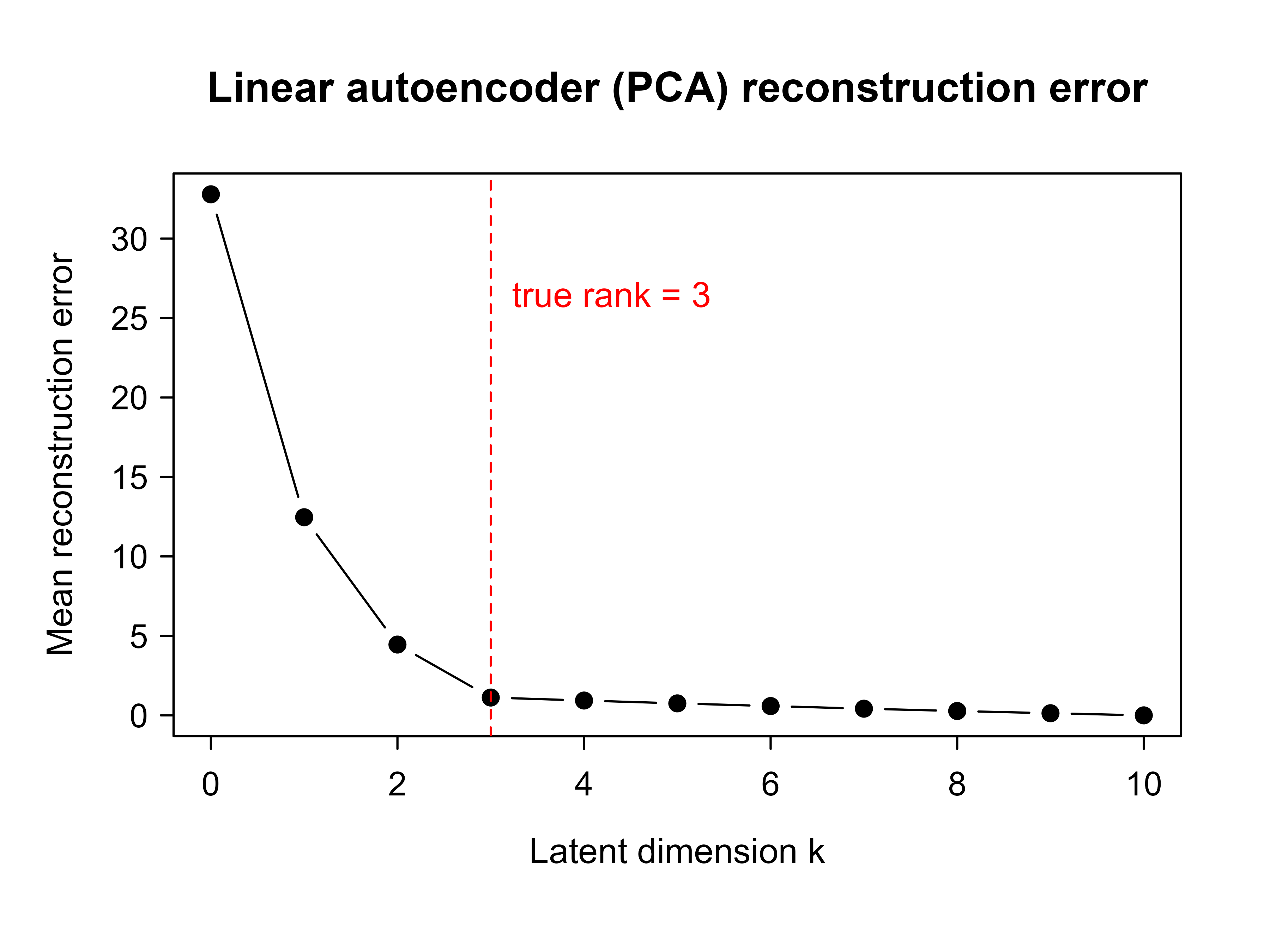
# SVD of the centered datasv<-svd(X_c)V<-sv$v# right singular vectors (principal directions)# Mean squared reconstruction error per observation for a given code size krecon_error<-function(k){if(k==0){Xhat<-matrix(0, nrow(X_c), ncol(X_c))}else{Vk<-V[, 1:k, drop =FALSE]Xhat<-X_c%*%Vk%*%t(Vk)# project then lift back}mean(rowSums((X_c-Xhat)^2))}ks<-0:perrors<-sapply(ks, recon_error)err_table<-data.frame( latent_dim_k =ks, reconstruction_error =round(errors, 4))err_table#> latent_dim_k reconstruction_error#> 1 0 32.7841#> 2 1 12.4651#> 3 2 4.4560#> 4 3 1.1217#> 5 4 0.9340#> 6 5 0.7546#> 7 6 0.5853#> 8 7 0.4210#> 9 8 0.2743#> 10 9 0.1343#> 11 10 0.0000
Reading down the table, the error drops sharply up to \(k = 3\), the true latent rank, and then flattens because the remaining components capture only noise. This is the signature of an undercomplete bottleneck matching the intrinsic dimension of the data: once the code is wide enough to hold the real structure, extra capacity buys almost nothing.
We can confirm that the SVD reconstruction agrees with prcomp and that the error equals the sum of the discarded eigenvalues, which is the closed form for the optimal linear reconstruction error.
Show code
# prcomp route should match the SVD route at, say, k = 3pc<-prcomp(X, center =TRUE, scale. =FALSE)k<-3scores_k<-pc$x[, 1:k, drop =FALSE]Xhat_pc<-scores_k%*%t(pc$rotation[, 1:k, drop =FALSE])err_prcomp<-mean(rowSums((X_c-Xhat_pc)^2))# Closed form: discarded variance = sum of squared singular values beyond k,# divided by n, summed over the dropped directionsd2<-sv$d^2err_closed<-sum(d2[(k+1):p])/nrow(X_c)c(svd_route =recon_error(k), prcomp_route =err_prcomp, closed_form =err_closed)#> svd_route prcomp_route closed_form #> 1.121718 1.121718 1.121718
The three numbers agree, which is the numerical statement of the Baldi and Hornik (1989) result: the best rank-\(k\) linear map is the PCA projection, and its reconstruction error is the variance left in the dropped directions. A trained linear autoencoder cannot do better than this, and at its optimum it does exactly this.
Finally we plot the reconstruction-error curve against the code dimension.
Show code
plot(ks, errors, type ="b", pch =19, xlab ="Latent dimension k", ylab ="Mean reconstruction error", main ="Linear autoencoder (PCA) reconstruction error")abline(v =r, lty =2, col ="red")text(r, max(errors)*0.8, labels ="true rank = 3", pos =4, col ="red")
Figure 41.1: Reconstruction error as a function of the latent code dimension k. The elbow at k = 3 matches the true latent rank of the data.
Figure 41.1 shows the resulting curve. The elbow at \(k = 3\) tells us how many code units a linear autoencoder needs to capture the data, and it lines up with the rank we built into the simulation. In practice you rarely know the true rank in advance, so reading the elbow off a curve like this is one way to choose the bottleneck size.
41.8 Sketch of a Nonlinear Autoencoder in Keras
The demonstration above stayed linear so it could run anywhere. To go beyond PCA you add nonlinear activations, and at that point the model is a genuine neural network that needs a deep-learning backend to train. The code below shows how a nonlinear undercomplete autoencoder is specified with Keras. It is not run here because the Python backend is not available in this build. The point of contrast with the demonstration above is the nonlinear activations, which let the model fit curved low-dimensional structure that the linear PCA reconstruction cannot.
Notice that the architecture mirrors the encoder-decoder picture from the start of the chapter: a stack of layers narrows down to a three-unit bottleneck, then a symmetric stack widens back out to the input dimension. The single change that lifts this above PCA is the relu activations, which let the encoder and decoder bend, so the code can trace curved low-dimensional structure that no straight projection can follow.
41.9 Summary
An autoencoder learns by reconstruction: it compresses an input into a code and rebuilds the input from it, and the value lies in what the bottleneck forces it to discard. When the encoder and decoder are linear, the result is PCA, a fact you verified numerically above. Nonlinear activations are what let autoencoders outrun PCA by fitting curved manifolds. When you want a wide code rather than a narrow one, regularization (denoising, sparsity, or contraction) takes over the job the bottleneck was doing, and the variational autoencoder turns the whole apparatus into a generative model by making the code a distribution instead of a point. From there the same trained network serves dimensionality reduction, pretraining, anomaly detection, and denoising.
41.10 Further Reading
The three works below are the foundational references for the results in this chapter.
Baldi and Hornik (1989) prove that a linear autoencoder under squared-error loss recovers the principal subspace and that its loss surface has no suboptimal local minima.
Hinton and Salakhutdinov (2006) show that deep nonlinear autoencoders, trained with a careful initialization, produce low-dimensional codes that outperform PCA for reconstruction and visualization.
Kingma and Welling (2014) introduce the variational autoencoder, the ELBO objective, and the reparameterization trick.
Baldi, Pierre, and Kurt Hornik. 1989. “Neural Networks and Principal Component Analysis: Learning from Examples Without Local Minima.”Neural Networks 2 (1): 53–58.
Hinton, Geoffrey E., and Ruslan R. Salakhutdinov. 2006. “Reducing the Dimensionality of Data with Neural Networks.”Science 313 (5786): 504–7.
Kingma, Diederik P., and Max Welling. 2014. “Auto-Encoding Variational Bayes.” In International Conference on Learning Representations (ICLR).
Vincent, Pascal. 2011. “A Connection Between Score Matching and Denoising Autoencoders.”Neural Computation 23 (7): 1661–74.
Most of the supervised methods in this book need labeled examples: an input paired with a known answer. Autoencoders need only the inputs themselves, which is why they belong to unsupervised learning alongside PCA and clustering.↩︎
Squared error is the natural loss for real-valued inputs. For binary or pixel-intensity inputs in \([0,1]\) a cross-entropy reconstruction loss is more common, but the logic is identical: reward faithful reconstruction.↩︎
The Kullback-Leibler divergence measures how far one probability is from another. Here it compares the observed average activation \(\hat{\rho}_j\) to the target \(\rho\) and grows whenever a unit fires far more or far less often than intended.↩︎
The Jacobian \(\partial f_\theta(x)/\partial x\) collects all the partial derivatives of the code with respect to the inputs. Its Frobenius norm is large when small input changes produce large code changes, so penalizing it asks the encoder to ignore directions that lead off the data.↩︎
Source Code
# Autoencoders and Representation Learning {#sec-autoencoders}```{r}#| include: falsesource("_common.R")```Imagine you had to describe a friend's face over the phone so that a sketch artist on the other end could draw it. You would not read off the color of every pixel. You would say a few things that matter: round face, dark curly hair, glasses, a small scar above the left eyebrow. From that short description the artist can reconstruct something close to the original. You have just done by hand what an autoencoder does automatically: compress a high-dimensional thing into a short summary, then rebuild it from that summary.An autoencoder is a neural network trained to copy its input to its output. That sounds pointless, because copying is trivial. The trick is that the network is forced to pass the data through a low-capacity intermediate representation, so the copying cannot be perfect. To reconstruct the input well despite that constraint, the network must learn what is worth keeping. What it learns to keep in that intermediate representation is a compressed code for the data. This makes the autoencoder a tool for representation learning, where the goal is to discover useful features without labels.^[Most of the supervised methods in this book need labeled examples: an input paired with a known answer. Autoencoders need only the inputs themselves, which is why they belong to *unsupervised* learning alongside PCA and clustering.]::: {.callout-important title="Key idea"}An autoencoder is not interesting because it can reconstruct the input. It is interesting because of *what it is forced to throw away* to do so. The discarded information is noise and redundancy; the retained information is the structure of the data.:::By the end of this chapter you will understand the encoder, the decoder, and the bottleneck that makes the whole thing work; you will see the precise sense in which a linear autoencoder is just PCA in disguise; you will meet the main regularized variants (denoising, sparse, contractive) and the variational autoencoder used for generation; and you will run a small demonstration in base R that confirms the linear-autoencoder-equals-PCA result numerically. Autoencoders sit next to the dimension reduction chapter (@sec-dimension-reduction) as the nonlinear generalization of the ideas you saw there.## Encoder, Decoder, and the BottleneckEvery autoencoder is built from two halves that work in opposite directions. The first half squeezes the data down into a short code; the second half tries to rebuild the original from that code. Training rewards the network when the rebuilt output matches the input.An autoencoder has two parts. The encoder maps an input $x \in \mathbb{R}^p$ to a code $z \in \mathbb{R}^k$,$$z = f_\theta(x),$$and the decoder maps the code back to the input space,$$\hat{x} = g_\phi(z).$$Training minimizes a reconstruction loss over the data. With squared error the objective is$$\min_{\theta, \phi} \; \sum_{i=1}^n \lVert x_i - g_\phi(f_\theta(x_i)) \rVert^2 .$$In words, we want the round trip from input to code and back to land as close to the original input as possible, averaged over the data.^[Squared error is the natural loss for real-valued inputs. For binary or pixel-intensity inputs in $[0,1]$ a cross-entropy reconstruction loss is more common, but the logic is identical: reward faithful reconstruction.]Everything then hinges on one number: the dimension $k$ of the code. It controls how much room the network has to store information, and therefore what it can and cannot do. There are two regimes to distinguish.- An undercomplete autoencoder has $k < p$. The code is smaller than the input, so the network cannot copy every input perfectly. It must use the limited capacity of the code to capture the structure that matters most for reconstruction. The layer that holds $z$ is called the bottleneck.- An overcomplete autoencoder has $k \ge p$. Here the code is at least as large as the input, and the network can learn the identity map and reconstruct everything with zero error. That solution is useless because it stores the data rather than a representation of it. Overcomplete autoencoders are only interesting when some form of regularization is added to stop the trivial copy.The bottleneck is the mechanism that turns a copy machine into a feature learner. By restricting how much information can flow from input to output, it forces the encoder to throw away noise and redundancy and keep the directions that explain the data.::: {.callout-tip title="Intuition"}Think of the bottleneck as a narrow doorway. If you must pass all your belongings through a doorway only $k$ items wide, you will carry the essentials and leave the clutter behind. The width $k$ decides how much detail survives the trip.:::::: {.callout-warning}An overcomplete autoencoder with no regularization will happily learn to do nothing useful, achieving zero reconstruction error by memorizing the identity. If you widen the code to $k \ge p$, you must add one of the constraints from the [Regularized Autoencoders] section, or the model learns nothing about the data.:::## Linear Autoencoders Recover the Principal SubspaceBefore reaching for nonlinear networks, it pays to ask what the simplest possible autoencoder learns. The answer is reassuring and clarifying: a linear autoencoder learns exactly the same thing as Principal Component Analysis. This is worth establishing carefully, because it tells us where the power of autoencoders actually comes from (the answer, given at the end of this section, is nonlinearity).The simplest autoencoder uses linear encoder and decoder with no nonlinear activations,$$z = W x, \qquad \hat{x} = U z = U W x,$$where $W$ is $k \times p$ and $U$ is $p \times k$. Assume the data are centered so that $\frac{1}{n}\sum_i x_i = 0$. The training objective is$$\min_{U, W} \; \sum_{i=1}^n \lVert x_i - U W x_i \rVert^2 .$$The key theoretical result, due to @baldi1989, is that the global minimum of this loss is reached when $U W$ equals the orthogonal projection onto the subspace spanned by the top $k$ principal components of the data. In other words, a linear autoencoder with squared-error loss learns the same subspace that PCA finds.::: {.callout-important title="Key idea"}A linear autoencoder is PCA wearing a neural-network costume. Training it by gradient descent and computing the top principal components are two routes to the same low-dimensional subspace.:::The reasoning is direct. The composed map $M = UW$ has rank at most $k$, so the problem is to find the rank-$k$ matrix $M$ that best reconstructs the centered data in squared error,$$\min_{\operatorname{rank}(M)\le k} \; \sum_{i=1}^n \lVert x_i - M x_i \rVert^2 .$$Let $X$ be the $n \times p$ matrix with the centered observations in its rows and let $\Sigma = \frac{1}{n} X^\top X$ be the sample covariance. The minimizing $M$ is the projection $M = V_k V_k^\top$, where $V_k$ holds the top $k$ eigenvectors of $\Sigma$, equivalently the top $k$ right singular vectors of $X$. This is the Eckart and Young low-rank approximation result, and it is exactly the rank-$k$ representation that PCA produces. See the dimension reduction chapter (@sec-dimension-reduction) for the PCA derivation through the singular value decomposition.#### Deriving the optimal reconstruction {#sec-autoencoders-eckartyoung}It is worth carrying the algebra through, because the derivation pins down both the optimal map and the residual error in closed form. Stacking the residuals into the matrix $X - XM^\top$ (each row is $x_i^\top - x_i^\top M^\top$), the objective is the squared Frobenius norm$$\sum_{i=1}^n \lVert x_i - M x_i \rVert^2 = \lVert X - X M^\top \rVert_F^2 .$$When $M = M^\top = P$ is a rank-$k$ orthogonal projector this is $\lVert X - XP \rVert_F^2 = \lVert X(I - P) \rVert_F^2$. Write the SVD $X = U_X D V^\top$ with singular values $d_1 \ge d_2 \ge \cdots \ge d_p \ge 0$. The Eckart and Young theorem states that among all matrices of rank at most $k$, the best Frobenius approximation of $X$ is its truncated SVD $X_k = U_X D_k V^\top$ obtained by zeroing all but the top $k$ singular values, and the residual is$$\min_{\operatorname{rank}(\hat X)\le k} \lVert X - \hat X \rVert_F^2 = \sum_{j=k+1}^{p} d_j^2 .$$ {#eq-autoencoders-eckartyoung}Any reconstruction of the form $XM^\top$ with $\operatorname{rank}(M)\le k$ has rank at most $k$, so it cannot beat the truncated SVD. The truncation is itself achieved by an orthogonal projector, since $X_k = X V_k V_k^\top$, so setting $M = V_k V_k^\top$ attains the bound. Dividing by $n$, the per-observation reconstruction error at the optimum is $\frac{1}{n}\sum_{j=k+1}^{p} d_j^2 = \sum_{j=k+1}^{p}\lambda_j$, the sum of the discarded eigenvalues $\lambda_j$ of $\Sigma$. This is precisely the closed form the demonstration below checks numerically.A short calculation explains why the projector form is optimal among symmetric candidates and clarifies the link to maximizing variance. For an orthogonal projector $P = V_k V_k^\top$,$$\lVert X(I - P) \rVert_F^2 = \operatorname{tr}\!\big((I-P) X^\top X (I-P)\big) = \operatorname{tr}(X^\top X) - \operatorname{tr}(P\, X^\top X),$$using $P^2 = P = P^\top$. Since $\operatorname{tr}(X^\top X)$ is fixed, minimizing reconstruction error is the same as maximizing $\operatorname{tr}(V_k^\top X^\top X V_k) = n \sum_{j} v_j^\top \Sigma\, v_j$ over orthonormal $V_k$, the total variance captured in the subspace. By the Ky Fan / Rayleigh-Ritz characterization this trace is maximized by the top $k$ eigenvectors of $\Sigma$, recovering PCA. The decoder $U$ need not equal $W^\top$ at the optimum, but @baldi1989 show that at any critical point the column space of $U$ coincides with an invariant subspace of $\Sigma$, and the global optimum selects the dominant one.Two points are worth stating precisely, because they are easy to get wrong.- The autoencoder recovers the span of the top $k$ principal components, not the components themselves. The factorization $M = UW$ is not unique because $UW = (UA)(A^{-1}W)$ for any invertible $A$. So the learned $W$ rows are some basis of the principal subspace, not necessarily orthonormal and not ordered by variance. PCA pins down a specific orthonormal ordered basis through the eigenvalue ordering, which the plain linear autoencoder does not impose.- @baldi1989 also showed that under squared-error loss the only local minima are global minima for this linear network. The loss surface has saddle points but no suboptimal local minima, which is why gradient descent on a linear autoencoder reliably finds the principal subspace.The practical message is that nonlinearity is what makes autoencoders more than PCA. A linear autoencoder cannot beat PCA. Once the encoder and decoder use nonlinear activations, the network can learn curved low-dimensional manifolds that no linear projection can represent.::: {.callout-tip title="When to use this"}If your data really do lie near a flat subspace, PCA is faster, has a closed-form solution, and gives you ordered, orthonormal components for free. Reach for a nonlinear autoencoder only when you have reason to believe the structure is curved, for example images, where a straight-line projection loses too much.:::## Regularized AutoencodersSo far the bottleneck has done all the work: a narrow code forces compression. But what if we want a code that is large, perhaps even larger than the input, yet still meaningful? As the warning above noted, a wide code with no other constraint just learns to copy. Regularized autoencoders solve this by adding a penalty or a constraint so that the network learns a useful representation even when the bottleneck alone would not force one. The three variants below differ only in *what* they penalize, and each encodes a different idea about what makes a representation good.### Denoising AutoencodersThe denoising autoencoder starts from a simple observation: if the network has to repair damage, it cannot get away with copying, because the thing it sees is no longer the thing it must produce.A denoising autoencoder corrupts the input and asks the network to reconstruct the clean version. Draw a corrupted input $\tilde{x}$ from a noise process $C(\tilde{x} \mid x)$, for example by adding Gaussian noise or by randomly zeroing entries, then train$$\min_{\theta, \phi} \; \mathbb{E}_{x}\, \mathbb{E}_{\tilde{x} \sim C(\cdot \mid x)} \; \lVert x - g_\phi(f_\theta(\tilde{x})) \rVert^2 .$$The network cannot simply copy because the input it sees is not the target it must produce. To remove noise it has to learn the structure of the clean data, which gives a representation that captures the data distribution rather than the identity map. This works even when the autoencoder is overcomplete.The denoising objective is not an arbitrary trick: under additive Gaussian corruption it is, in the small-noise limit, an estimator of the score of the data density. Suppose $\tilde x = x + \sigma\varepsilon$ with $\varepsilon \sim \mathcal{N}(0,I)$, and let $r(\tilde x) = g_\phi(f_\theta(\tilde x))$ denote the reconstruction. The population denoising risk is $\mathbb{E}\,\lVert x - r(\tilde x) \rVert^2$. For a fixed corrupted point, the conditional expectation $\mathbb{E}[x \mid \tilde x]$ is the minimizer of squared error, and Tweedie's formula gives it in closed form in terms of the marginal density $p_\sigma(\tilde x)$ of the corrupted data,$$\mathbb{E}[x \mid \tilde x] = \tilde x + \sigma^2 \,\nabla_{\tilde x} \log p_\sigma(\tilde x).$$ {#eq-autoencoders-tweedie}To derive @eq-autoencoders-tweedie, write $p_\sigma(\tilde x) = \int p(x)\,\mathcal{N}(\tilde x; x, \sigma^2 I)\,dx$ and differentiate. Because $\nabla_{\tilde x}\mathcal{N}(\tilde x; x, \sigma^2 I) = -\sigma^{-2}(\tilde x - x)\,\mathcal{N}(\tilde x; x, \sigma^2 I)$,$$\nabla_{\tilde x} \log p_\sigma(\tilde x) = \frac{\nabla_{\tilde x} p_\sigma(\tilde x)}{p_\sigma(\tilde x)} = \frac{\int p(x)\,(-\sigma^{-2})(\tilde x - x)\,\mathcal{N}(\tilde x; x, \sigma^2 I)\,dx}{p_\sigma(\tilde x)} = \sigma^{-2}\big(\mathbb{E}[x \mid \tilde x] - \tilde x\big),$$which rearranges to @eq-autoencoders-tweedie. Therefore the optimal reconstruction satisfies $r^\star(\tilde x) - \tilde x = \sigma^2 \nabla_{\tilde x}\log p_\sigma(\tilde x)$: the residual a trained denoiser produces points back toward the data manifold along the gradient of the log density. This is the basis of denoising score matching (@vincent2011) and the reason denoising autoencoders connect directly to modern score-based and diffusion generative models. The same identity explains why a denoiser learns the data distribution rather than the identity even when overcomplete: the best it can do is report the noise-aware posterior mean, which encodes $p$.::: {.callout-tip title="Intuition"}Filling in a smudged word in a sentence requires understanding the sentence. Forcing the network to undo corruption forces it to learn how the data are supposed to look, which is exactly the structure we want it to capture.:::### Sparse AutoencodersThe sparse autoencoder takes a different angle. Instead of corrupting the input, it limits how many code units may switch on for any single example. A sparse autoencoder adds a penalty on the code activations so that only a few units are active for any given input. With an $L_1$ penalty the objective is$$\min_{\theta, \phi} \; \sum_{i=1}^n \lVert x_i - g_\phi(z_i) \rVert^2 + \lambda \lVert z_i \rVert_1 ,$$where $z_i = f_\theta(x_i)$. The $L_1$ penalty pushes most entries of the code to exactly zero, so each input is explained by a handful of active units. An alternative penalty drives the average activation of each unit toward a small target $\rho$ (the desired activation rate, for example $0.05$) using a Kullback and Leibler term.^[The Kullback-Leibler divergence measures how far one probability is from another. Here it compares the observed average activation $\hat{\rho}_j$ to the target $\rho$ and grows whenever a unit fires far more or far less often than intended.] If $\hat{\rho}_j$ is the mean activation of unit $j$ over the data, the penalty is$$\sum_{j=1}^k \mathrm{KL}(\rho \,\Vert\, \hat{\rho}_j) = \sum_{j=1}^k \left[ \rho \log \frac{\rho}{\hat{\rho}_j} + (1-\rho) \log \frac{1-\rho}{1-\hat{\rho}_j} \right] .$$ {#eq-autoencoders-sparse-kl}Sparsity lets the code be large while keeping each example explained by a few active features, which tends to produce parts-based and interpretable representations. For a face, one unit might respond to a nose, another to an eyebrow, rather than every unit firing a little for everything.### Contractive AutoencodersThe contractive autoencoder regularizes a third property: stability. It penalizes the sensitivity of the code to small changes in the input, so that wiggling the input a little barely moves the code. A contractive autoencoder penalizes the sensitivity of the code to small changes in the input. The penalty is the squared Frobenius norm of the encoder Jacobian,$$\min_{\theta, \phi} \; \sum_{i=1}^n \lVert x_i - g_\phi(f_\theta(x_i)) \rVert^2 + \lambda \left\lVert \frac{\partial f_\theta(x_i)}{\partial x} \right\rVert_F^2 .$$This pushes the encoder to be flat in most directions and to respond only along the directions in which the data actually vary, so the learned representation is locally invariant to small perturbations off the data manifold.^[The Jacobian $\partial f_\theta(x)/\partial x$ collects all the partial derivatives of the code with respect to the inputs. Its Frobenius norm is large when small input changes produce large code changes, so penalizing it asks the encoder to ignore directions that lead off the data.]For a single-layer encoder $z_j = s(a_j)$ with pre-activation $a = Wx + b$ and elementwise nonlinearity $s$, the Jacobian penalty has a cheap closed form that avoids ever forming the full matrix. Since $\partial z_j / \partial x_l = s'(a_j)\, W_{jl}$,$$\left\lVert \frac{\partial f_\theta(x)}{\partial x} \right\rVert_F^2 = \sum_{j=1}^k \sum_{l=1}^p \big(s'(a_j)\,W_{jl}\big)^2 = \sum_{j=1}^k s'(a_j)^2 \sum_{l=1}^p W_{jl}^2 = \sum_{j=1}^k s'(a_j)^2 \,\lVert W_{j\cdot} \rVert^2 .$$ {#eq-autoencoders-cae-jacobian}For the logistic sigmoid, $s'(a_j) = z_j(1 - z_j)$, so the penalty is $\sum_j z_j^2 (1-z_j)^2 \lVert W_{j\cdot}\rVert^2$, computable in $O(kp)$ from quantities already available in the forward pass. Two contrasts sharpen the intuition. Against weight decay, which penalizes $\lVert W \rVert_F^2$ uniformly and is data-independent, @eq-autoencoders-cae-jacobian weights each row by the local activation slope $s'(a_j)^2$, so it relaxes the penalty exactly where a unit is saturated and active on the data and tightens it elsewhere. Against the denoising autoencoder, a first-order Taylor expansion of the reconstruction shows that training with small additive Gaussian corruption is, to leading order in $\sigma^2$, equivalent to penalizing the Jacobian of the whole reconstruction $g_\phi \circ f_\theta$; the contractive penalty instead targets the encoder Jacobian directly, making the connection explicit rather than implicit.To summarize the three: denoising asks the code to survive corruption, sparsity asks it to use few units at a time, and contraction asks it to stay still under small input nudges. All three break the trivial-copy solution, which is what lets an overcomplete autoencoder learn something real.## Variational AutoencodersEvery autoencoder so far has been a deterministic compressor: feed in $x$, get back one code $z$. The variational autoencoder changes the question from "how do I compress this?" to "how was this data generated?" That shift lets it not only compress but also *generate* brand-new examples by sampling codes and decoding them.A variational autoencoder (VAE) is a generative latent-variable model rather than a deterministic compressor. It assumes data are produced by sampling a latent code $z$ from a prior $p(z)$, usually a standard normal, then sampling $x$ from a decoder distribution $p_\phi(x \mid z)$. We would like to fit the parameters by maximizing the marginal likelihood $\log p(x)$, but that integral over $z$ is intractable.The VAE introduces an approximate posterior $q_\theta(z \mid x)$, the encoder, and optimizes a lower bound on the log likelihood called the evidence lower bound (ELBO),$$\log p(x) \ge \mathbb{E}_{q_\theta(z \mid x)}\big[\log p_\phi(x \mid z)\big] - \mathrm{KL}\big(q_\theta(z \mid x) \,\Vert\, p(z)\big).$$The first term rewards reconstructing $x$ from codes drawn from the encoder, and plays the role of the reconstruction loss. The second term pulls the encoder distribution toward the prior, which regularizes the latent space so that nearby codes decode to similar inputs and the space can be sampled to generate new data.#### Deriving the ELBO {#sec-autoencoders-elbo}The bound is not assumed; it follows from a single algebraic identity. Multiply and divide inside the log-marginal by the encoder $q_\theta(z\mid x)$ and apply Jensen's inequality to the concave logarithm,$$\log p(x) = \log \int p_\phi(x\mid z)\,p(z)\,dz = \log \mathbb{E}_{q_\theta(z\mid x)}\!\left[\frac{p_\phi(x\mid z)\,p(z)}{q_\theta(z\mid x)}\right] \ge \mathbb{E}_{q_\theta(z\mid x)}\!\left[\log \frac{p_\phi(x\mid z)\,p(z)}{q_\theta(z\mid x)}\right].$$Splitting the logarithm separates a reconstruction term from a prior-matching term,$$\mathbb{E}_{q_\theta}\big[\log p_\phi(x\mid z)\big] + \mathbb{E}_{q_\theta}\!\left[\log \frac{p(z)}{q_\theta(z\mid x)}\right] = \mathbb{E}_{q_\theta}\big[\log p_\phi(x\mid z)\big] - \mathrm{KL}\big(q_\theta(z\mid x)\,\Vert\,p(z)\big),$$which is the ELBO. The gap in the inequality is exactly the posterior approximation error: a direct expansion gives$$\log p(x) - \mathrm{ELBO}(x) = \mathrm{KL}\big(q_\theta(z\mid x)\,\Vert\,p(z\mid x)\big) \ge 0,$$ {#eq-autoencoders-elbo-gap}so maximizing the ELBO simultaneously raises a bound on the likelihood and tightens the encoder toward the true posterior $p(z\mid x)$. The bound is exact precisely when $q_\theta(z\mid x) = p(z\mid x)$.With a Gaussian encoder $q_\theta = \mathcal{N}(\mu, \operatorname{diag}(\sigma^2))$ and standard normal prior $p(z) = \mathcal{N}(0, I)$ in dimension $k$, the KL term has a closed form that needs no sampling,$$\mathrm{KL}\big(q_\theta(z\mid x)\,\Vert\,p(z)\big) = \frac{1}{2}\sum_{j=1}^{k}\Big(\mu_j^2 + \sigma_j^2 - \log \sigma_j^2 - 1\Big).$$ {#eq-autoencoders-vae-kl}This is the standard KL between two diagonal Gaussians evaluated at unit prior variance and zero prior mean; each coordinate contributes a penalty that is zero only when $\mu_j = 0$ and $\sigma_j = 1$, that is, when the posterior coordinate already matches the prior. Only the reconstruction term needs the Monte Carlo estimate via the reparameterized sample, which is why a VAE trains with a single (or a few) noise draws per example. A practical failure mode follows directly from @eq-autoencoders-vae-kl: when the decoder is powerful enough to model $x$ without using $z$, the optimizer can drive the KL to zero by setting $\mu_j = 0, \sigma_j = 1$, ignoring the input. This is posterior collapse, mitigated by KL warm-up (annealing a weight on the KL term from zero) or by weakening the decoder.::: {.callout-tip title="Intuition"}The two ELBO terms are in tension, and that tension is the whole point. Reconstruction wants each input to claim its own private corner of the latent space; the KL term wants every input to look like a draw from the same standard normal. The compromise is a latent space that is both faithful and smooth, smooth enough that sampling a random $z$ and decoding it yields a plausible new example.:::To train by gradient descent we need gradients through the sampling step $z \sim q_\theta(z \mid x)$. The reparameterization trick rewrites the sample as a deterministic function of the parameters and an external noise variable. With a Gaussian encoder $q_\theta(z \mid x) = \mathcal{N}(\mu_\theta(x), \operatorname{diag}(\sigma_\theta^2(x)))$, write$$z = \mu_\theta(x) + \sigma_\theta(x) \odot \epsilon, \qquad \epsilon \sim \mathcal{N}(0, I),$$where $\odot$ is elementwise multiplication. The randomness now lives in $\epsilon$, which does not depend on the parameters, so gradients flow through $\mu_\theta$ and $\sigma_\theta$. This is the construction of @kingma2014.::: {.callout-note}You cannot backpropagate through a coin flip. Sampling $z$ directly blocks the gradient because the random draw has no derivative with respect to the parameters. The reparameterization trick sidesteps this by moving the randomness into $\epsilon$, an input the network does not control, leaving a smooth deterministic path from the parameters to $z$.:::This is only a brief introduction. The full treatment of VAEs, including the decoder likelihood choices and the connection to other generative models, belongs with the generative models material (@sec-generative-models).## What Autoencoders Are Used ForThe pieces above come together in four recurring applications. Each one reuses the same trained network but reads a different part of it: some use the code, one uses the reconstruction error, one uses the output directly.- Dimensionality reduction. The bottleneck code is a low-dimensional representation. A nonlinear autoencoder can capture curved structure that PCA misses, which is the point of @hinton2006.- Pretraining. An encoder trained on unlabeled data gives features that can initialize or feed a supervised model, useful when labels are scarce.- Anomaly detection (@sec-anomaly-detection). Train the autoencoder on normal data only. Normal inputs reconstruct with small error, while anomalous inputs that do not match the learned structure reconstruct poorly. The reconstruction error $\lVert x - \hat{x} \rVert^2$ becomes an anomaly score.- Denoising. A denoising autoencoder maps corrupted inputs to clean ones, so it can be used directly to clean up noisy signals or images.::: {.callout-tip}Anomaly detection is the most common practical use and the easiest to deploy. You need only normal data to train, and the anomaly score is just the reconstruction error, with no labels and no threshold tuning beyond picking a cutoff.:::## Practical Considerations and TheoryThe variants above share a common set of design decisions and failure modes. This section collects the properties that govern how an autoencoder behaves in practice and how to set its knobs.### Choosing and diagnosing the code dimensionThe single most consequential hyperparameter is the bottleneck width $k$, because it sets the capacity of the representation. For the linear model the optimal reconstruction error is the closed form $\sum_{j>k}\lambda_j$ derived in @eq-autoencoders-eckartyoung, so the reconstruction-error-versus-$k$ curve is exactly the cumulative tail of the eigenvalue spectrum and its elbow estimates the intrinsic dimension. For nonlinear autoencoders no such closed form exists, but the same diagnostic curve applies: train at several values of $k$ and look for the elbow where added capacity stops reducing held-out reconstruction error. Use held-out, not training, error, because a sufficiently wide nonlinear autoencoder can drive training error toward zero by memorizing, the nonlinear analogue of the overcomplete identity map. A nonlinear autoencoder can in principle reconstruct $n$ training points exactly with a code as narrow as $k=1$, since a sufficiently wiggly encoder can map each point to a distinct real number and the decoder can invert it; this is overfitting through the bottleneck rather than around it, and it is why a capacity bound from $k$ alone is not a generalization guarantee.### Regularization strength and other knobsEach regularized variant adds one penalty weight whose scale must be tuned, typically by held-out reconstruction error or by a downstream task.- Denoising: the noise level $\sigma$ (or the masking probability) is the effective regularizer. Small $\sigma$ recovers the ordinary autoencoder; large $\sigma$ forces stronger reliance on data structure but eventually destroys the signal. As @eq-autoencoders-tweedie shows, $\sigma$ also sets the scale at which the denoiser estimates the score, so it trades resolution against stability.- Sparse: the penalty weight $\lambda$ and, for the KL form, the target rate $\rho$ (often $0.01$ to $0.05$). The KL penalty in @eq-autoencoders-sparse-kl refers to mean activations, so it requires either full-batch or a running estimate of $\hat\rho_j$ across a minibatch.- Contractive: the weight $\lambda$ on the Jacobian penalty of @eq-autoencoders-cae-jacobian. Because the penalty is computed per minibatch in $O(kp)$ for a single layer, it is cheap for shallow encoders but scales with the number of layers when the full deep Jacobian is used.- Variational: the optional weight $\beta$ on the KL term of @eq-autoencoders-vae-kl (the $\beta$-VAE). Raising $\beta$ above one buys a more disentangled, prior-conforming latent space at the cost of reconstruction fidelity; lowering it risks losing the generative smoothness that makes sampling work.### Computational cost and connectionsTraining cost is dominated by the forward and backward passes through encoder and decoder, $O(\text{layer widths})$ per example per step, identical to a feedforward network of the same architecture; the autoencoder is unusual only in that its target is its input. Two structural connections are worth keeping in view. First, with linear maps and squared error the autoencoder collapses to PCA exactly (the result derived above), so any departure from PCA performance is attributable to nonlinearity or regularization, not to the autoencoder framing itself. Second, tying the decoder weights to the encoder ($U = W^\top$) halves the parameter count and is a common default; at the linear optimum this is automatically consistent with an orthonormal-basis solution but in the nonlinear case it is a genuine constraint that can help or hurt depending on the architecture.::: {.callout-warning}A low reconstruction error is necessary but not sufficient for a useful code. An overcomplete or over-flexible autoencoder can reconstruct perfectly while learning a representation that is no more informative than the raw input. Always evaluate the code on the downstream purpose (separability, anomaly ranking, generative sample quality), not on reconstruction error alone.:::## Demonstration: Linear Autoencoder Equals PCAWe will now turn the central theoretical result into numbers you can check. If a linear autoencoder really does learn the PCA subspace, then PCA must produce exactly the reconstruction error that a perfectly trained linear autoencoder would reach. We can verify that without training any network at all.The runnable demonstration below confirms the central theoretical result in base R. We do not train a neural network. Instead we use the fact that the optimal linear autoencoder reconstruction is the rank-$k$ PCA projection, so PCA gives us the reconstruction error that an ideally trained linear autoencoder would reach.We generate data with low-dimensional structure, compute PCA two ways (through `prcomp` and through the SVD), reconstruct from the top $k$ components, and tabulate the reconstruction error as a function of the code dimension $k$. The plan is to build data that secretly lives near a 3-dimensional subspace, then watch the reconstruction error collapse exactly when the code reaches dimension 3.We start by simulating the data. Three latent factors are mixed by random loadings to fill ten observed dimensions, then a small amount of noise is added so the structure is approximate rather than exact.```{r ae-data}set.seed(1301)n <-500# observationsp <-10# ambient dimensionr <-3# true latent rank# Latent factors and random loadings give data that lives near a 3D subspaceZ <-matrix(rnorm(n * r), n, r)B <-matrix(rnorm(r * p), r, p)signal <- Z %*% Bnoise <-matrix(rnorm(n * p, sd =0.4), n, p)X <- signal + noise# Center the data, which the linear-autoencoder = PCA result assumesX_c <-scale(X, center =TRUE, scale =FALSE)dim(X_c)```Now reconstruct from the top $k$ principal components. The reconstruction is $\hat{X} = X_c V_k V_k^\top$, where $V_k$ holds the top $k$ right singular vectors. This $V_k V_k^\top$ is exactly the projection $UW$ that an optimal linear autoencoder learns.```{r ae-recon}# SVD of the centered datasv <-svd(X_c)V <- sv$v # right singular vectors (principal directions)# Mean squared reconstruction error per observation for a given code size krecon_error <-function(k) {if (k ==0) { Xhat <-matrix(0, nrow(X_c), ncol(X_c)) } else { Vk <- V[, 1:k, drop =FALSE] Xhat <- X_c %*% Vk %*%t(Vk) # project then lift back }mean(rowSums((X_c - Xhat)^2))}ks <-0:perrors <-sapply(ks, recon_error)err_table <-data.frame(latent_dim_k = ks,reconstruction_error =round(errors, 4))err_table```Reading down the table, the error drops sharply up to $k = 3$, the true latent rank, and then flattens because the remaining components capture only noise. This is the signature of an undercomplete bottleneck matching the intrinsic dimension of the data: once the code is wide enough to hold the real structure, extra capacity buys almost nothing.We can confirm that the SVD reconstruction agrees with `prcomp` and that the error equals the sum of the discarded eigenvalues, which is the closed form for the optimal linear reconstruction error.```{r ae-check}# prcomp route should match the SVD route at, say, k = 3pc <-prcomp(X, center =TRUE, scale. =FALSE)k <-3scores_k <- pc$x[, 1:k, drop =FALSE]Xhat_pc <- scores_k %*%t(pc$rotation[, 1:k, drop =FALSE])err_prcomp <-mean(rowSums((X_c - Xhat_pc)^2))# Closed form: discarded variance = sum of squared singular values beyond k,# divided by n, summed over the dropped directionsd2 <- sv$d^2err_closed <-sum(d2[(k +1):p]) /nrow(X_c)c(svd_route =recon_error(k),prcomp_route = err_prcomp,closed_form = err_closed)```The three numbers agree, which is the numerical statement of the @baldi1989 result: the best rank-$k$ linear map is the PCA projection, and its reconstruction error is the variance left in the dropped directions. A trained linear autoencoder cannot do better than this, and at its optimum it does exactly this.Finally we plot the reconstruction-error curve against the code dimension.```{r fig-autoencoders-recon-error-curve, fig.width=6, fig.height=4.5, fig.cap="Reconstruction error as a function of the latent code dimension k. The elbow at k = 3 matches the true latent rank of the data."}plot(ks, errors, type ="b", pch =19,xlab ="Latent dimension k",ylab ="Mean reconstruction error",main ="Linear autoencoder (PCA) reconstruction error")abline(v = r, lty =2, col ="red")text(r, max(errors) *0.8, labels ="true rank = 3",pos =4, col ="red")```@fig-autoencoders-recon-error-curve shows the resulting curve. The elbow at $k = 3$ tells us how many code units a linear autoencoder needs to capture the data, and it lines up with the rank we built into the simulation. In practice you rarely know the true rank in advance, so reading the elbow off a curve like this is one way to choose the bottleneck size.## Sketch of a Nonlinear Autoencoder in KerasThe demonstration above stayed linear so it could run anywhere. To go beyond PCA you add nonlinear activations, and at that point the model is a genuine neural network that needs a deep-learning backend to train. The code below shows how a nonlinear undercomplete autoencoder is specified with Keras. It is not run here because the Python backend is not available in this build. The point of contrast with the demonstration above is the nonlinear activations, which let the model fit curved low-dimensional structure that the linear PCA reconstruction cannot.```{r ae-keras, eval=FALSE}library(keras)input_dim <-10code_dim <-3inputs <-layer_input(shape = input_dim)code <- inputs |>layer_dense(units =16, activation ="relu") |>layer_dense(units = code_dim, activation ="relu", name ="bottleneck")outputs <- code |>layer_dense(units =16, activation ="relu") |>layer_dense(units = input_dim, activation ="linear")autoencoder <-keras_model(inputs, outputs)autoencoder |>compile(optimizer ="adam", loss ="mse")# autoencoder |> fit(X, X, epochs = 50, batch_size = 32)```Notice that the architecture mirrors the encoder-decoder picture from the start of the chapter: a stack of layers narrows down to a three-unit `bottleneck`, then a symmetric stack widens back out to the input dimension. The single change that lifts this above PCA is the `relu` activations, which let the encoder and decoder bend, so the code can trace curved low-dimensional structure that no straight projection can follow.## SummaryAn autoencoder learns by reconstruction: it compresses an input into a code and rebuilds the input from it, and the value lies in what the bottleneck forces it to discard. When the encoder and decoder are linear, the result is PCA, a fact you verified numerically above. Nonlinear activations are what let autoencoders outrun PCA by fitting curved manifolds. When you want a wide code rather than a narrow one, regularization (denoising, sparsity, or contraction) takes over the job the bottleneck was doing, and the variational autoencoder turns the whole apparatus into a generative model by making the code a distribution instead of a point. From there the same trained network serves dimensionality reduction, pretraining, anomaly detection, and denoising.## Further ReadingThe three works below are the foundational references for the results in this chapter.- @baldi1989 prove that a linear autoencoder under squared-error loss recovers the principal subspace and that its loss surface has no suboptimal local minima.- @hinton2006 show that deep nonlinear autoencoders, trained with a careful initialization, produce low-dimensional codes that outperform PCA for reconstruction and visualization.- @kingma2014 introduce the variational autoencoder, the ELBO objective, and the reparameterization trick.