Imagine you have written a careful script that holds out some data, fits one model, and reports its error. It works. Then a colleague asks you to compare ten models, each with a different preprocessing recipe, each tuned over a handful of settings, all judged fairly on the same data splits. Suddenly your tidy script becomes a sprawl of copy-pasted loops, and somewhere in that sprawl it is easy to accidentally let the test data influence the training step, which quietly inflates every number you report. The mlr3 ecosystem exists to make that whole comparison routine, repeatable, and hard to get wrong.
The mlr3 ecosystem is a modern, object oriented framework for machine learning in R.1 It is the successor to the older mlr package, rebuilt on top of R6 classes and data.table for speed and a consistent interface. The name stands for “machine learning in R, version 3”. This chapter explains the building blocks (tasks, learners, measures), the pipeline system (mlr3pipelines), automated tuning (mlr3tuning), and benchmarking, then contrasts the design with tidymodels. By the end you should understand not just the mlr3 syntax but the underlying workflow that any serious comparison of models needs, regardless of which framework you use.
Key idea
A model comparison is only honest if every candidate is evaluated under identical conditions and no information from the held out data ever reaches the training step. Everything mlr3 does is in service of those two rules.
Because mlr3 is probably not installed in your environment, the mlr3 specific code chunks are marked eval=FALSE. They are written to be correct and current, so you can copy them into a session that has mlr3 installed. To teach the core ideas with code that actually runs, the chapter also includes a base R implementation of the resampling and benchmarking loop that mlr3 automates, so you can see exactly what the framework is doing under the hood.
91.1 Where this fits in a modern workflow
A supervised learning project repeats the same skeleton regardless of the algorithm: hold out data for honest evaluation, fit a model on the training portion, predict on the held out portion, score the predictions, and compare candidate models under identical conditions. Doing this by hand for one model is easy. Doing it consistently across a dozen models, several preprocessing variants, and a hyperparameter search, without leaking information from the test set into training, is where bookkeeping errors creep in.
mlr3 exists to remove that bookkeeping. Its central design move is to give each concept in the skeleton above its own first class object, so that the parts can be mixed and matched. The four core objects are the following.
A task bundles the data with its prediction target and metadata (which column is the outcome, which are features, what the problem type is).
A learner wraps a fitting algorithm behind a uniform $train() and $predict() interface, so a random forest and a penalized regression look the same to the surrounding code.
A measure is a scoring function such as classification error or root mean squared error.
A resampling describes how to split the data (cross validation, holdout, bootstrap).
The payoff of separating these concerns is that they become interchangeable. Because a learner is just an object that exposes $train() and $predict(), you can swap one for another without touching the evaluation code, attach preprocessing as a reusable graph, and run an apples to apples benchmark. In a larger AI or ML engineering setting this matters because the same task and resampling can be reused across experiments, logged, and handed to a tuning routine, which keeps the comparison fair and reproducible.
Intuition
Think of the four objects as standardized plugs and sockets. As long as every learner has the same shape of plug, you can swap which algorithm is plugged into your evaluation harness without rewiring anything else.
With the vocabulary in place, we can look at the three foundational objects in code.
91.2 Tasks, learners, and measures
A task fixes the supervised learning problem: it answers “what are we predicting, from what, and what kind of prediction is it?” For a regression task with target \(y\) and feature vector \(x \in \mathbb{R}^p\), the goal is to learn a function \(\hat{f}: \mathbb{R}^p \to \mathbb{R}\) that maps features to a numeric prediction. For classification the target is categorical and the learner may produce either class labels or class probabilities.
Show code
library(mlr3)library(mlr3learners)# A regression task: predict median house value from the mtcars-like exampletask<-as_task_regr(mtcars, target ="mpg", id ="cars")task# prints target, features, and number of rows# A learner is an algorithm wrapped behind a uniform interfacelearner<-lrn("regr.ranger", num.trees =500)# A measure scores predictionsmeasure<-msr("regr.rmse")# Manual train / predict on an explicit splitset.seed(1)split<-partition(task, ratio =0.7)# train / test row idslearner$train(task, row_ids =split$train)pred<-learner$predict(task, row_ids =split$test)pred$score(measure)# RMSE on the held out rows
The key idea is that task, learner, and measure are independent. To try a different algorithm you change only the lrn(...) line; the splitting, training, prediction, and scoring code stays exactly as it is. The naming convention is lrn("<type>.<algorithm>"), for example regr.ranger, classif.xgboost, or classif.log_reg. You can list everything available with mlr_learners and as.data.table(mlr_learners).
Tip
The prefix before the dot is the task type (regr for regression, classif for classification) and the part after the dot names the underlying R package or algorithm. If lrn("classif.ranger") complains that it cannot find the learner, the usual cause is that the mlr3learners package, or the backing package such as ranger, is not loaded.
A measure is just a function of the prediction object and the truth: it takes what the model predicted and what actually happened, and returns a single number summarizing the gap. For regression the root mean squared error over a held out set of size \(m\) is
In words, RMSE penalizes large numeric misses heavily because the errors are squared, and log loss rewards a classifier for being confident and right while punishing it severely for being confident and wrong.2
91.2.1 Resampling and the math it estimates
We now have a way to score a model on one held out set. But a single split is a coin flip: a lucky split can make a mediocre model look good. Resampling is the practice of splitting many times and averaging, and it is the heart of honest evaluation. The goal is to estimate how well a learner generalizes to data it has never seen, the central concern of the model performance chapter (Chapter 82).
Let \(L(y, \hat{f}(x))\) be a loss. The quantity we care about is the expected loss on a fresh observation drawn from the same distribution,
where \(\hat{f}\) was trained on a sample. We cannot compute this expectation, so we estimate it by repeatedly splitting the data into a part used for training and a disjoint part used for scoring. In \(K\) fold cross validation the data are partitioned into \(K\) roughly equal folds. For fold \(k\) the model is trained on all other folds and scored on fold \(k\), giving an estimate
where \(D_k\) is the set of rows in fold \(k\) and \(\hat{f}^{(-k)}\) is the model trained with fold \(k\) removed. The disjointness of training and scoring rows is what makes this an honest estimate rather than an optimistic one.
Intuition
Every row gets to be a test point exactly once, judged by a model that never saw it during training. Averaging the \(K\) scores uses all the data for both purposes without ever letting a row grade its own homework.
In mlr3 this entire procedure is one object plus one call.
Show code
# 5 fold cross validation, fully described as an objectresampling<-rsmp("cv", folds =5)rr<-resample(task, learner, resampling)rr$aggregate(msr("regr.rmse"))# mean RMSE across foldsrr$score(msr("regr.rmse"))# per fold RMSE
91.3 A runnable base R analogue of the resampling and benchmark loop
It is easy to treat resample() and benchmark() as magic. They are not. The following chunk runs, and it implements in plain base R exactly what those functions do: a \(K\) fold cross validation loop that scores several learners on the same folds. Reading it once makes the rest of the chapter feel like convenience wrappers rather than new concepts. Notice the trick that keeps the comparison fair: we generate one set of fold assignments and reuse it for every learner, which removes split to split noise from the comparison so any difference in scores reflects the models, not luck of the draw.
Show code
set.seed(123)# A simple regression problem with a known structuren<-300x1<-rnorm(n); x2<-rnorm(n); x3<-rnorm(n)y<-2*x1-1.5*x2+0.5*x1*x2+rnorm(n, sd =1)dat<-data.frame(y, x1, x2, x3)# Define a uniform "learner" interface: each is a list with fit() and predict()learners<-list( ols =list( fit =function(train)lm(y~., data =train), predict =function(model, newdata)predict(model, newdata)), ols_interact =list( fit =function(train)lm(y~x1*x2+x3, data =train), predict =function(model, newdata)predict(model, newdata)), mean_only =list( fit =function(train)mean(train$y), predict =function(model, newdata)rep(model, nrow(newdata))))rmse<-function(truth, pred)sqrt(mean((truth-pred)^2))# One set of folds, shared across all learners (the core fairness idea)K<-5folds<-sample(rep(1:K, length.out =n))# Resample-and-benchmark loopresults<-data.frame()for(lnameinnames(learners)){lr<-learners[[lname]]fold_rmse<-numeric(K)for(kin1:K){train<-dat[folds!=k, ]test<-dat[folds==k, ]model<-lr$fit(train)preds<-lr$predict(model, test)fold_rmse[k]<-rmse(test$y, preds)}results<-rbind(results,data.frame(learner =lname, mean_rmse =mean(fold_rmse), se_rmse =sd(fold_rmse)/sqrt(K)))}results<-results[order(results$mean_rmse), ]print(results, row.names =FALSE)#> learner mean_rmse se_rmse#> ols_interact 1.028901 0.03421155#> ols 1.110769 0.02721009#> mean_only 2.595046 0.11054147
Reading the output table, the model with the interaction term wins, because the data generating process includes an \(x_1 x_2\) term that the plain additive model cannot represent, and the intercept only baseline (mean_only, which always predicts the training mean) is worst, as it should be. That baseline is not pointless: it tells us the floor. Any model that cannot beat it has learned nothing. The mean_rmse column is the cross validation estimate \(\widehat{\text{Err}}_{CV}\) from the formula above, and se_rmse is a rough standard error across folds that tells you how much to trust the differences.3 In mlr3 this entire loop collapses to a single benchmark() call over a grid of tasks, learners, and resamplings, which we will see at the end of the chapter.
91.3.1 A figure: the cross validation estimate across folds
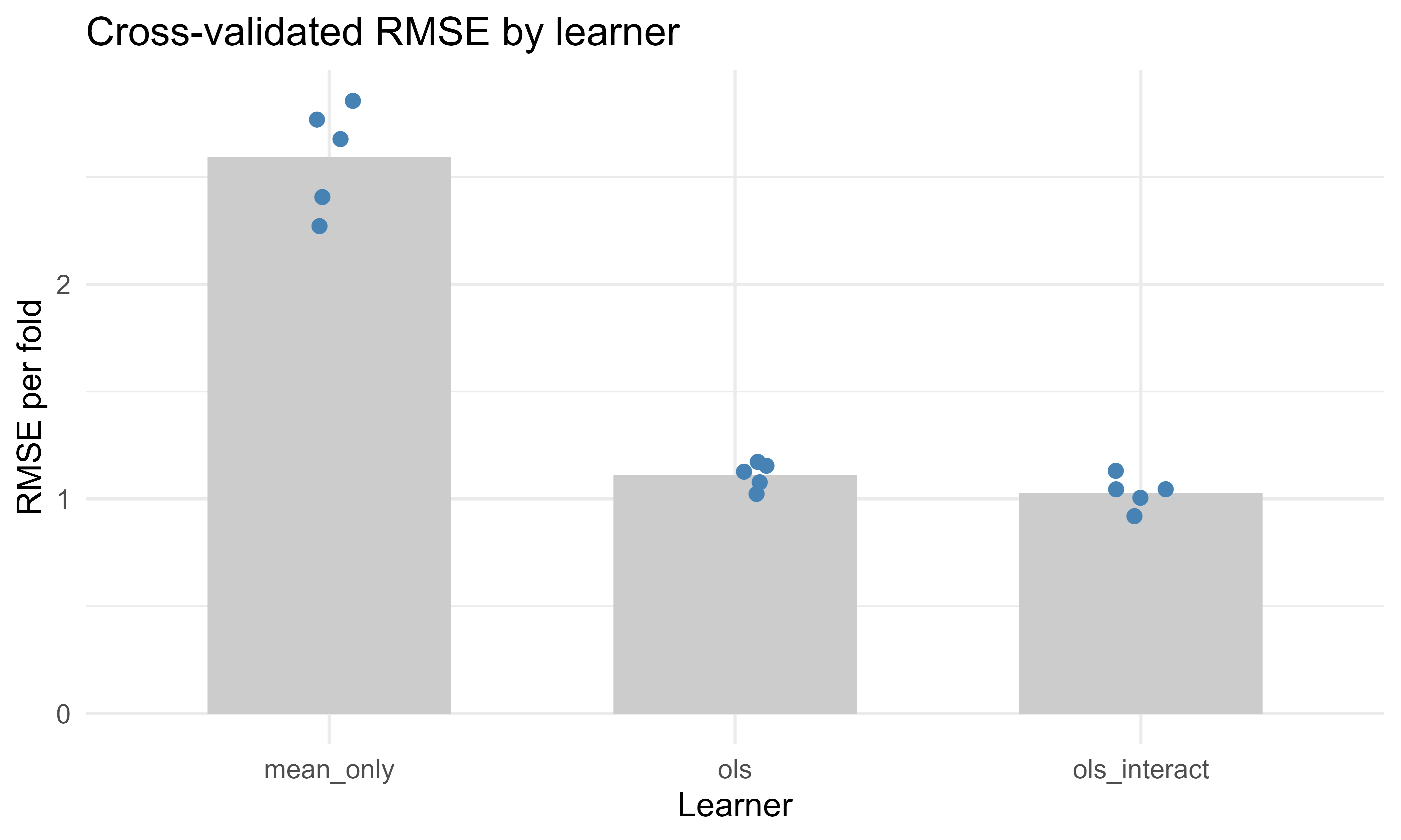
Figure 91.1 makes the spread behind those averages visible: each point is one fold’s RMSE and the grey bar is the cross-validated mean, so you can judge at a glance whether a gap between learners is comfortably larger than the fold-to-fold scatter.
Show code
# Recompute per-fold values so we can show their spreaddetail<-data.frame()for(lnameinnames(learners)){lr<-learners[[lname]]for(kin1:K){train<-dat[folds!=k, ]test<-dat[folds==k, ]model<-lr$fit(train)preds<-lr$predict(model, test)detail<-rbind(detail,data.frame(learner =lname, fold =k, rmse =rmse(test$y, preds)))}}library(ggplot2)agg<-aggregate(rmse~learner, detail, mean)ggplot(detail, aes(x =learner, y =rmse))+geom_col(data =agg, aes(x =learner, y =rmse), fill ="grey80", width =0.6)+geom_jitter(width =0.08, height =0, size =2, colour ="steelblue")+labs(x ="Learner", y ="RMSE per fold", title ="Cross-validated RMSE by learner")+theme_minimal(base_size =12)
Figure 91.1: Per-fold RMSE for three learners under shared 5-fold cross validation. Points are folds and the bar is the cross-validated mean.
91.4 Pipelines with mlr3pipelines
Real data is rarely ready to model. It needs preprocessing: imputation of missing values, encoding of categorical factors into numbers, scaling features to comparable ranges, feature selection. Here lurks one of the most common and most invisible mistakes in applied machine learning. If you learn a preprocessing rule from the whole data set, for example the mean used to center a feature, then that rule has already peeked at the rows you intend to hold out, and your cross validation estimate becomes optimistic. The fix is to treat preprocessing as part of the model, so that every step is refit inside each training fold and never sees the test rows.
Warning
Centering, scaling, imputing, or selecting features on the full data set before you split is leakage. It is tempting because it is convenient, and it silently makes every reported score too good. The whole point of a pipeline is to make the correct thing the easy thing.
mlr3pipelines represents the full model, preprocessing included, as a directed graph of PipeOp objects (short for pipeline operators). Each PipeOp has a $train() and $predict() step, mirroring a learner, which is exactly what lets preprocessing be refit per fold. Connecting operators with the %>>% operator builds a Graph, and wrapping the graph as a GraphLearner produces something that behaves exactly like an ordinary learner, so it slots into resampling and tuning unchanged.
Show code
library(mlr3pipelines)library(mlr3learners)graph<-po("imputemedian")%>>%# impute numeric NAs by training-fold medianpo("scale")%>>%# standardize using training-fold statisticspo("encode")%>>%# one-hot encode factorslrn("classif.xgboost", nrounds =200)glrn<-as_learner(graph)# now behaves like any other learner# Because preprocessing lives inside the graph, statistics are recomputed# on each training fold during resampling, which prevents leakageglrn$train(task)
The leakage point deserves a concrete example. Suppose you standardize a feature using its mean \(\bar{x}\) and standard deviation \(s\) computed on the full data set, then cross validate. The test fold rows contributed to \(\bar{x}\) and \(s\), so the scaled test features already encode information about the held out rows, and the held out set is no longer truly held out. With a pipeline, \(\bar{x}\) and \(s\) are estimated only on the training rows of each fold and then applied to that fold’s test rows, which keeps the estimate honest. This is the same disjointness principle from cross validation, now extended to cover preprocessing as well as model fitting.
91.5 Tuning with mlr3tuning
Most learners have hyperparameters: settings that the training algorithm does not learn from the data and that you must choose yourself, such as the number of trees in a forest, the learning rate of a boosting model, or the strength of a regularization penalty. Different choices can change performance dramatically, so we search for good ones. Tuning is that search, framed as an optimization problem over configurations to minimize the resampled loss. Let \(\lambda\) be a hyperparameter configuration and \(\widehat{\text{Err}}_{CV}(\lambda)\) the cross validated loss for a learner configured with \(\lambda\). Tuning solves
over a search space \(\Lambda\). The strategies differ only in how they explore that space: grid search evaluates a fixed lattice of points, random search samples points at random (often more efficient when only a few hyperparameters matter), and Bayesian optimization fits a surrogate model of \(\widehat{\text{Err}}_{CV}(\lambda)\) to predict which configurations are worth trying next. The hyperparameter optimization chapter (Chapter 84) covers these search strategies in more depth.
Note
Random search frequently beats grid search for the same budget, because grids waste evaluations on dimensions that do not matter, while random sampling spreads its trials across the dimensions that do. Bayesian optimization adds a layer of intelligence on top of that by learning from the trials it has already run.
Now for the subtle point that trips up even experienced practitioners. Tuning is itself part of model fitting, because the data is what chose \(\lambda^*\). So if you report the best inner cross validation score as your model’s performance, you are reporting a number that was chosen because it was the best, which makes it optimistic almost by definition. To get an unbiased estimate you must wrap the tuning inside an outer resampling loop. This is called nested resampling: an inner loop selects \(\lambda^*\), and an outer loop scores the whole tuning procedure on data the inner loop never saw.
Warning
The single most common way to overstate a model’s accuracy is to tune on cross validation and then report the best cross validation score as the final number. The same data both chose and judged the configuration. Nested resampling is the cure, and mlr3 makes it a one-liner via auto_tuner inside an outer resample().
Show code
library(mlr3tuning)library(paradox)# Define the search space with the modern ps() / to_tune() stylelearner<-lrn("classif.xgboost", nrounds =to_tune(50, 500), eta =to_tune(1e-3, 0.3, logscale =TRUE), max_depth =to_tune(2, 8))# An auto-tuning learner: tuning happens inside trainingat<-auto_tuner( tuner =tnr("random_search"), learner =learner, resampling =rsmp("cv", folds =3), # inner loop measure =msr("classif.logloss"), term_evals =40)# Nested resampling: the outer loop scores the entire tuning procedureouter<-rsmp("cv", folds =5)# outer looprr<-resample(task, at, outer, store_models =TRUE)rr$aggregate(msr("classif.logloss"))# unbiased estimate
91.6 Benchmarking many learners at once
We can now return to the comparison problem that motivated the chapter. Benchmarking runs a grid of (task, learner, resampling) combinations and collects all scores in one table, with every learner evaluated on the same splits. This is the structured, leakage-safe version of the base R loop from earlier, except that the learners can be full GraphLearner pipelines and auto-tuners, and the bookkeeping is handled for you.
Show code
design<-benchmark_grid( tasks =task, learners =list(lrn("classif.featureless"), # baselinelrn("classif.log_reg"),lrn("classif.ranger"),lrn("classif.xgboost")), resamplings =rsmp("cv", folds =5))bmr<-benchmark(design)bmr$aggregate(msr("classif.auc"))# one row per learner, shared foldsautoplot(bmr)# boxplot of per-fold scores
91.7 Comparison to tidymodels
If you have read the tidymodels material elsewhere in this book (Chapter 90), you may be wondering how the two frameworks relate. The short answer is that they solve the same problem in the same spirit and differ mainly in taste. Both mlr3 and tidymodels prevent leakage by treating preprocessing as part of the model, and both delegate parallelism to the same future backend. The visible difference is programming style. mlr3 uses R6 mutable objects with $train() and $predict() methods, which feels like classic object oriented programming where you call methods on objects that hold state. tidymodels uses a functional, pipe friendly style built around the tidyverse, where objects are immutable and you compose verbs into a workflow. Table 91.1 lines up the corresponding pieces of each framework so you can translate a workflow from one to the other.
Table 91.1: Correspondence between the core building blocks of the mlr3 and tidymodels frameworks.
Concept
mlr3
tidymodels
Problem definition
Task (e.g. as_task_classif)
implicit in the formula and data passed to functions
Algorithm wrapper
Learner via lrn("classif.ranger")
parsnip model spec, e.g. rand_forest()
Preprocessing
mlr3pipelinesPipeOp graph
recipes recipe
Model plus preprocessing
GraphLearner
workflow
Resampling
rsmp("cv") from mlr3
rsample (vfold_cv)
Tuning
mlr3tuning plus paradox search space
tune plus dials
Metrics
Measure via msr(...)
yardstick
Object model
mutable R6 classes
immutable, functional, tidyverse
Parallel backend
future
future
Ensembling and stacking
mlr3pipelines graphs
stacks
A useful way to think about the choice: if you already live in the tidyverse and like pipes of immutable objects, tidymodels will feel natural. If you want a compact object graph where learners, pipelines, and tuners are all interchangeable objects you can store, clone, and pass around, mlr3 will feel natural. Neither is faster or more correct in principle; both delegate parallelism to future and both protect against leakage when used as intended.
The base R loop earlier in this chapter is the conceptual common denominator of both. Each defines a uniform fit and predict interface, fixes a set of folds, and scores every candidate on the same folds.
91.8 Practical guidance, pitfalls, and when to use it
When to use this
Reach for mlr3 when you need to compare many models or preprocessing variants under identical, reproducible conditions, when you want preprocessing bundled into the model so that resampling stays honest, or when you want automated tuning with nested resampling done correctly. It is well suited to research style benchmarking and to ML engineering pipelines where the same task and resampling objects are reused across experiments. For a quick one-off fit of a single model, the framework’s machinery is more than you need.
Most of the ways these workflows go wrong are variations on the two rules from the start of the chapter: keep test data out of training, and judge every model under identical conditions. The recurring pitfalls below are all special cases.
Preprocessing outside the resampling loop. Scaling, imputing, or selecting features on the full data set before cross validation leaks the test folds into training. Always wrap preprocessing in a GraphLearner so it refits per fold.
Tuning without nested resampling. Reporting the best inner cross validation score as the model’s performance is optimistic, because the same data both chose and judged the configuration. Use auto_tuner inside an outer resample().
Different splits per learner. Comparing models that were each evaluated on their own random splits confounds the model with the split. Reuse one resampling object across the whole benchmark, as benchmark_grid does automatically.
Forgetting a baseline. Always include a trivial learner (classif.featureless or regr.featureless) so you know the floor; a model that cannot beat predicting the mean or majority class is not learning anything.
Reading too much into a single fold. Look at the per fold spread, not just the aggregate, and use repeated cross validation when folds are noisy.
To tie it all together, here is a reasonable default workflow. Define the task, build a GraphLearner with the needed preprocessing, set up a five or ten fold resampling, benchmark a small set of learners plus a baseline, then tune the winner with auto_tuner under nested resampling before reporting its score. Follow that sequence and the honesty of your numbers is built in rather than hoped for.
Key idea
Everything in this chapter, in mlr3 or in the base R loop, comes down to a uniform fit-and-predict interface, a fixed set of folds shared across candidates, and preprocessing and tuning kept strictly inside the training side of each split. Master that pattern and the specific framework becomes a detail.
91.9 Further reading
Lang, Binder, Richter, Schratz, Pfisterer, Coors, Au, Casalicchio, Kotthoff, and Bischl (2019). “mlr3: A modern object-oriented machine learning framework in R.” Journal of Open Source Software.
Bischl, Sonabend, Kotthoff, and Lang, editors (2024). “Applied Machine Learning Using mlr3 in R.” CRC Press. Available online as the mlr3book.
Binder, Pfisterer, Lang, Schneider, Kotthoff, and Bischl (2021). “mlr3pipelines: Flexible machine learning pipelines in R.” Journal of Machine Learning Research.
Kuhn and Silge (2022). “Tidy Modeling with R.” O’Reilly. The reference for the tidymodels comparison.
Hastie, Tibshirani, and Friedman (2009). “The Elements of Statistical Learning,” second edition. Springer. For the underlying theory of cross validation and model assessment in Chapter 7.
Object oriented here means the framework is organized around “objects” that carry both data and the methods that act on them. A learner object, for instance, knows how to train itself and how to predict, so you call learner$train(...) rather than passing the model through a chain of standalone functions.↩︎
Log loss goes to infinity as the predicted probability of the true class goes to zero, which is why a single confidently-wrong prediction can dominate the score. This is a feature, not a bug: it discourages overconfidence.↩︎
A standard error roughly the size of the gap between two learners is a hint that the difference may be noise rather than signal. Repeated cross validation, which reruns the whole split-and-score procedure with fresh fold assignments, gives a more stable comparison.↩︎
Source Code
# The mlr3 Ecosystem {#sec-mlr3-ecosystem}```{r}#| include: falsesource("_common.R")```Imagine you have written a careful script that holds out some data, fits one model, and reports its error. It works. Then a colleague asks you to compare ten models, each with a different preprocessing recipe, each tuned over a handful of settings, all judged fairly on the same data splits. Suddenly your tidy script becomes a sprawl of copy-pasted loops, and somewhere in that sprawl it is easy to accidentally let the test data influence the training step, which quietly inflates every number you report. The `mlr3` ecosystem exists to make that whole comparison routine, repeatable, and hard to get wrong.The `mlr3` ecosystem is a modern, object oriented framework for machine learning in R.^[Object oriented here means the framework is organized around "objects" that carry both data and the methods that act on them. A learner object, for instance, knows how to train itself and how to predict, so you call `learner$train(...)` rather than passing the model through a chain of standalone functions.] It is the successor to the older `mlr` package, rebuilt on top of `R6` classes and `data.table` for speed and a consistent interface. The name stands for "machine learning in R, version 3". This chapter explains the building blocks (tasks, learners, measures), the pipeline system (`mlr3pipelines`), automated tuning (`mlr3tuning`), and benchmarking, then contrasts the design with `tidymodels`. By the end you should understand not just the `mlr3` syntax but the underlying workflow that any serious comparison of models needs, regardless of which framework you use.::: {.callout-important title="Key idea"}A model comparison is only honest if every candidate is evaluated under identical conditions and no information from the held out data ever reaches the training step. Everything `mlr3` does is in service of those two rules.:::Because `mlr3` is probably not installed in your environment, the `mlr3` specific code chunks are marked `eval=FALSE`. They are written to be correct and current, so you can copy them into a session that has `mlr3` installed. To teach the core ideas with code that actually runs, the chapter also includes a base R implementation of the resampling and benchmarking loop that `mlr3` automates, so you can see exactly what the framework is doing under the hood.## Where this fits in a modern workflowA supervised learning project repeats the same skeleton regardless of the algorithm: hold out data for honest evaluation, fit a model on the training portion, predict on the held out portion, score the predictions, and compare candidate models under identical conditions. Doing this by hand for one model is easy. Doing it consistently across a dozen models, several preprocessing variants, and a hyperparameter search, without leaking information from the test set into training, is where bookkeeping errors creep in.`mlr3` exists to remove that bookkeeping. Its central design move is to give each concept in the skeleton above its own first class object, so that the parts can be mixed and matched. The four core objects are the following.- A task bundles the data with its prediction target and metadata (which column is the outcome, which are features, what the problem type is).- A learner wraps a fitting algorithm behind a uniform `$train()` and `$predict()` interface, so a random forest and a penalized regression look the same to the surrounding code.- A measure is a scoring function such as classification error or root mean squared error.- A resampling describes how to split the data (cross validation, holdout, bootstrap).The payoff of separating these concerns is that they become interchangeable. Because a learner is just an object that exposes `$train()` and `$predict()`, you can swap one for another without touching the evaluation code, attach preprocessing as a reusable graph, and run an apples to apples benchmark. In a larger AI or ML engineering setting this matters because the same task and resampling can be reused across experiments, logged, and handed to a tuning routine, which keeps the comparison fair and reproducible.::: {.callout-tip title="Intuition"}Think of the four objects as standardized plugs and sockets. As long as every learner has the same shape of plug, you can swap which algorithm is plugged into your evaluation harness without rewiring anything else.:::With the vocabulary in place, we can look at the three foundational objects in code.## Tasks, learners, and measuresA task fixes the supervised learning problem: it answers "what are we predicting, from what, and what kind of prediction is it?" For a regression task with target $y$ and feature vector $x \in \mathbb{R}^p$, the goal is to learn a function $\hat{f}: \mathbb{R}^p \to \mathbb{R}$ that maps features to a numeric prediction. For classification the target is categorical and the learner may produce either class labels or class probabilities.```{r mlr3-basics, eval=FALSE}library(mlr3)library(mlr3learners)# A regression task: predict median house value from the mtcars-like exampletask <-as_task_regr(mtcars, target ="mpg", id ="cars")task # prints target, features, and number of rows# A learner is an algorithm wrapped behind a uniform interfacelearner <-lrn("regr.ranger", num.trees =500)# A measure scores predictionsmeasure <-msr("regr.rmse")# Manual train / predict on an explicit splitset.seed(1)split <-partition(task, ratio =0.7) # train / test row idslearner$train(task, row_ids = split$train)pred <- learner$predict(task, row_ids = split$test)pred$score(measure) # RMSE on the held out rows```The key idea is that `task`, `learner`, and `measure` are independent. To try a different algorithm you change only the `lrn(...)` line; the splitting, training, prediction, and scoring code stays exactly as it is. The naming convention is `lrn("<type>.<algorithm>")`, for example `regr.ranger`, `classif.xgboost`, or `classif.log_reg`. You can list everything available with `mlr_learners` and `as.data.table(mlr_learners)`.::: {.callout-tip}The prefix before the dot is the task type (`regr` for regression, `classif` for classification) and the part after the dot names the underlying R package or algorithm. If `lrn("classif.ranger")` complains that it cannot find the learner, the usual cause is that the `mlr3learners` package, or the backing package such as `ranger`, is not loaded.:::A measure is just a function of the prediction object and the truth: it takes what the model predicted and what actually happened, and returns a single number summarizing the gap. For regression the root mean squared error over a held out set of size $m$ is$$\text{RMSE} = \sqrt{\frac{1}{m} \sum_{i=1}^{m} \left( y_i - \hat{f}(x_i) \right)^2 } .$$For classification with predicted probabilities $\hat{p}_i$ for the positive class and labels $y_i \in \{0,1\}$, the log loss is$$\text{LogLoss} = -\frac{1}{m} \sum_{i=1}^{m} \left[ y_i \log \hat{p}_i + (1 - y_i) \log (1 - \hat{p}_i) \right] .$$In words, RMSE penalizes large numeric misses heavily because the errors are squared, and log loss rewards a classifier for being confident and right while punishing it severely for being confident and wrong.^[Log loss goes to infinity as the predicted probability of the true class goes to zero, which is why a single confidently-wrong prediction can dominate the score. This is a feature, not a bug: it discourages overconfidence.]### Resampling and the math it estimatesWe now have a way to score a model on one held out set. But a single split is a coin flip: a lucky split can make a mediocre model look good. Resampling is the practice of splitting many times and averaging, and it is the heart of honest evaluation. The goal is to estimate how well a learner generalizes to data it has never seen, the central concern of the model performance chapter (@sec-model-performance).Let $L(y, \hat{f}(x))$ be a loss. The quantity we care about is the expected loss on a fresh observation drawn from the same distribution,$$\text{Err} = \mathbb{E}_{(x,y)} \left[ L\big(y, \hat{f}(x)\big) \right],$$where $\hat{f}$ was trained on a sample. We cannot compute this expectation, so we estimate it by repeatedly splitting the data into a part used for training and a disjoint part used for scoring. In $K$ fold cross validation the data are partitioned into $K$ roughly equal folds. For fold $k$ the model is trained on all other folds and scored on fold $k$, giving an estimate$$\widehat{\text{Err}}_{CV} = \frac{1}{K} \sum_{k=1}^{K} \frac{1}{|D_k|} \sum_{i \in D_k} L\big(y_i, \hat{f}^{(-k)}(x_i)\big),$$where $D_k$ is the set of rows in fold $k$ and $\hat{f}^{(-k)}$ is the model trained with fold $k$ removed. The disjointness of training and scoring rows is what makes this an honest estimate rather than an optimistic one.::: {.callout-tip title="Intuition"}Every row gets to be a test point exactly once, judged by a model that never saw it during training. Averaging the $K$ scores uses all the data for both purposes without ever letting a row grade its own homework.:::In `mlr3` this entire procedure is one object plus one call.```{r mlr3-resample, eval=FALSE}# 5 fold cross validation, fully described as an objectresampling <-rsmp("cv", folds =5)rr <-resample(task, learner, resampling)rr$aggregate(msr("regr.rmse")) # mean RMSE across foldsrr$score(msr("regr.rmse")) # per fold RMSE```## A runnable base R analogue of the resampling and benchmark loopIt is easy to treat `resample()` and `benchmark()` as magic. They are not. The following chunk runs, and it implements in plain base R exactly what those functions do: a $K$ fold cross validation loop that scores several learners on the same folds. Reading it once makes the rest of the chapter feel like convenience wrappers rather than new concepts. Notice the trick that keeps the comparison fair: we generate one set of fold assignments and reuse it for every learner, which removes split to split noise from the comparison so any difference in scores reflects the models, not luck of the draw.```{r base-cv-benchmark}set.seed(123)# A simple regression problem with a known structuren <-300x1 <-rnorm(n); x2 <-rnorm(n); x3 <-rnorm(n)y <-2* x1 -1.5* x2 +0.5* x1 * x2 +rnorm(n, sd =1)dat <-data.frame(y, x1, x2, x3)# Define a uniform "learner" interface: each is a list with fit() and predict()learners <-list(ols =list(fit =function(train) lm(y ~ ., data = train),predict =function(model, newdata) predict(model, newdata) ),ols_interact =list(fit =function(train) lm(y ~ x1 * x2 + x3, data = train),predict =function(model, newdata) predict(model, newdata) ),mean_only =list(fit =function(train) mean(train$y),predict =function(model, newdata) rep(model, nrow(newdata)) ))rmse <-function(truth, pred) sqrt(mean((truth - pred)^2))# One set of folds, shared across all learners (the core fairness idea)K <-5folds <-sample(rep(1:K, length.out = n))# Resample-and-benchmark loopresults <-data.frame()for (lname innames(learners)) { lr <- learners[[lname]] fold_rmse <-numeric(K)for (k in1:K) { train <- dat[folds != k, ] test <- dat[folds == k, ] model <- lr$fit(train) preds <- lr$predict(model, test) fold_rmse[k] <-rmse(test$y, preds) } results <-rbind( results,data.frame(learner = lname,mean_rmse =mean(fold_rmse),se_rmse =sd(fold_rmse) /sqrt(K)) )}results <- results[order(results$mean_rmse), ]print(results, row.names =FALSE)```Reading the output table, the model with the interaction term wins, because the data generating process includes an $x_1 x_2$ term that the plain additive model cannot represent, and the intercept only baseline (`mean_only`, which always predicts the training mean) is worst, as it should be. That baseline is not pointless: it tells us the floor. Any model that cannot beat it has learned nothing. The `mean_rmse` column is the cross validation estimate $\widehat{\text{Err}}_{CV}$ from the formula above, and `se_rmse` is a rough standard error across folds that tells you how much to trust the differences.^[A standard error roughly the size of the gap between two learners is a hint that the difference may be noise rather than signal. Repeated cross validation, which reruns the whole split-and-score procedure with fresh fold assignments, gives a more stable comparison.] In `mlr3` this entire loop collapses to a single `benchmark()` call over a grid of tasks, learners, and resamplings, which we will see at the end of the chapter.### A figure: the cross validation estimate across folds@fig-mlr3-ecosystem-cv-rmse makes the spread behind those averages visible: each point is one fold's RMSE and the grey bar is the cross-validated mean, so you can judge at a glance whether a gap between learners is comfortably larger than the fold-to-fold scatter.```{r fig-mlr3-ecosystem-cv-rmse, fig.cap="Per-fold RMSE for three learners under shared 5-fold cross validation. Points are folds and the bar is the cross-validated mean.", fig.width=7, fig.height=4.2}# Recompute per-fold values so we can show their spreaddetail <-data.frame()for (lname innames(learners)) { lr <- learners[[lname]]for (k in1:K) { train <- dat[folds != k, ] test <- dat[folds == k, ] model <- lr$fit(train) preds <- lr$predict(model, test) detail <-rbind(detail,data.frame(learner = lname, fold = k, rmse =rmse(test$y, preds))) }}library(ggplot2)agg <-aggregate(rmse ~ learner, detail, mean)ggplot(detail, aes(x = learner, y = rmse)) +geom_col(data = agg, aes(x = learner, y = rmse),fill ="grey80", width =0.6) +geom_jitter(width =0.08, height =0, size =2, colour ="steelblue") +labs(x ="Learner", y ="RMSE per fold",title ="Cross-validated RMSE by learner") +theme_minimal(base_size =12)```## Pipelines with mlr3pipelinesReal data is rarely ready to model. It needs preprocessing: imputation of missing values, encoding of categorical factors into numbers, scaling features to comparable ranges, feature selection. Here lurks one of the most common and most invisible mistakes in applied machine learning. If you learn a preprocessing rule from the whole data set, for example the mean used to center a feature, then that rule has already peeked at the rows you intend to hold out, and your cross validation estimate becomes optimistic. The fix is to treat preprocessing as part of the model, so that every step is refit inside each training fold and never sees the test rows.::: {.callout-warning}Centering, scaling, imputing, or selecting features on the full data set before you split is leakage. It is tempting because it is convenient, and it silently makes every reported score too good. The whole point of a pipeline is to make the correct thing the easy thing.:::`mlr3pipelines` represents the full model, preprocessing included, as a directed graph of `PipeOp` objects (short for pipeline operators). Each `PipeOp` has a `$train()` and `$predict()` step, mirroring a learner, which is exactly what lets preprocessing be refit per fold. Connecting operators with the `%>>%` operator builds a `Graph`, and wrapping the graph as a `GraphLearner` produces something that behaves exactly like an ordinary learner, so it slots into resampling and tuning unchanged.```{r mlr3-pipeline, eval=FALSE}library(mlr3pipelines)library(mlr3learners)graph <-po("imputemedian") %>>%# impute numeric NAs by training-fold medianpo("scale") %>>%# standardize using training-fold statisticspo("encode") %>>%# one-hot encode factorslrn("classif.xgboost", nrounds =200)glrn <-as_learner(graph) # now behaves like any other learner# Because preprocessing lives inside the graph, statistics are recomputed# on each training fold during resampling, which prevents leakageglrn$train(task)```The leakage point deserves a concrete example. Suppose you standardize a feature using its mean $\bar{x}$ and standard deviation $s$ computed on the full data set, then cross validate. The test fold rows contributed to $\bar{x}$ and $s$, so the scaled test features already encode information about the held out rows, and the held out set is no longer truly held out. With a pipeline, $\bar{x}$ and $s$ are estimated only on the training rows of each fold and then applied to that fold's test rows, which keeps the estimate honest. This is the same disjointness principle from cross validation, now extended to cover preprocessing as well as model fitting.## Tuning with mlr3tuningMost learners have hyperparameters: settings that the training algorithm does not learn from the data and that you must choose yourself, such as the number of trees in a forest, the learning rate of a boosting model, or the strength of a regularization penalty. Different choices can change performance dramatically, so we search for good ones. Tuning is that search, framed as an optimization problem over configurations to minimize the resampled loss. Let $\lambda$ be a hyperparameter configuration and $\widehat{\text{Err}}_{CV}(\lambda)$ the cross validated loss for a learner configured with $\lambda$. Tuning solves$$\lambda^* = \arg\min_{\lambda \in \Lambda} \widehat{\text{Err}}_{CV}(\lambda),$$over a search space $\Lambda$. The strategies differ only in how they explore that space: grid search evaluates a fixed lattice of points, random search samples points at random (often more efficient when only a few hyperparameters matter), and Bayesian optimization fits a surrogate model of $\widehat{\text{Err}}_{CV}(\lambda)$ to predict which configurations are worth trying next. The hyperparameter optimization chapter (@sec-hyperparameter-optimization) covers these search strategies in more depth.::: {.callout-note}Random search frequently beats grid search for the same budget, because grids waste evaluations on dimensions that do not matter, while random sampling spreads its trials across the dimensions that do. Bayesian optimization adds a layer of intelligence on top of that by learning from the trials it has already run.:::Now for the subtle point that trips up even experienced practitioners. Tuning is itself part of model fitting, because the data is what chose $\lambda^*$. So if you report the best inner cross validation score as your model's performance, you are reporting a number that was chosen because it was the best, which makes it optimistic almost by definition. To get an unbiased estimate you must wrap the tuning inside an outer resampling loop. This is called nested resampling: an inner loop selects $\lambda^*$, and an outer loop scores the whole tuning procedure on data the inner loop never saw.::: {.callout-warning}The single most common way to overstate a model's accuracy is to tune on cross validation and then report the best cross validation score as the final number. The same data both chose and judged the configuration. Nested resampling is the cure, and `mlr3` makes it a one-liner via `auto_tuner` inside an outer `resample()`.:::```{r mlr3-tuning, eval=FALSE}library(mlr3tuning)library(paradox)# Define the search space with the modern ps() / to_tune() stylelearner <-lrn("classif.xgboost",nrounds =to_tune(50, 500),eta =to_tune(1e-3, 0.3, logscale =TRUE),max_depth =to_tune(2, 8))# An auto-tuning learner: tuning happens inside trainingat <-auto_tuner(tuner =tnr("random_search"),learner = learner,resampling =rsmp("cv", folds =3), # inner loopmeasure =msr("classif.logloss"),term_evals =40)# Nested resampling: the outer loop scores the entire tuning procedureouter <-rsmp("cv", folds =5) # outer looprr <-resample(task, at, outer, store_models =TRUE)rr$aggregate(msr("classif.logloss")) # unbiased estimate```## Benchmarking many learners at onceWe can now return to the comparison problem that motivated the chapter. Benchmarking runs a grid of (task, learner, resampling) combinations and collects all scores in one table, with every learner evaluated on the same splits. This is the structured, leakage-safe version of the base R loop from earlier, except that the learners can be full `GraphLearner` pipelines and auto-tuners, and the bookkeeping is handled for you.```{r mlr3-benchmark, eval=FALSE}design <-benchmark_grid(tasks = task,learners =list(lrn("classif.featureless"), # baselinelrn("classif.log_reg"),lrn("classif.ranger"),lrn("classif.xgboost") ),resamplings =rsmp("cv", folds =5))bmr <-benchmark(design)bmr$aggregate(msr("classif.auc")) # one row per learner, shared foldsautoplot(bmr) # boxplot of per-fold scores```## Comparison to tidymodelsIf you have read the tidymodels material elsewhere in this book (@sec-tidymodels-framework), you may be wondering how the two frameworks relate. The short answer is that they solve the same problem in the same spirit and differ mainly in taste. Both `mlr3` and `tidymodels` prevent leakage by treating preprocessing as part of the model, and both delegate parallelism to the same `future` backend. The visible difference is programming style. `mlr3` uses `R6` mutable objects with `$train()` and `$predict()` methods, which feels like classic object oriented programming where you call methods on objects that hold state. `tidymodels` uses a functional, pipe friendly style built around the tidyverse, where objects are immutable and you compose verbs into a workflow. @tbl-mlr3-ecosystem-framework-map lines up the corresponding pieces of each framework so you can translate a workflow from one to the other.| Concept | mlr3 | tidymodels ||---|---|---|| Problem definition |`Task` (e.g. `as_task_classif`) | implicit in the formula and data passed to functions || Algorithm wrapper |`Learner` via `lrn("classif.ranger")`|`parsnip` model spec, e.g. `rand_forest()`|| Preprocessing |`mlr3pipelines``PipeOp` graph |`recipes` recipe || Model plus preprocessing |`GraphLearner`|`workflow`|| Resampling |`rsmp("cv")` from `mlr3`|`rsample` (`vfold_cv`) || Tuning |`mlr3tuning` plus `paradox` search space |`tune` plus `dials`|| Metrics |`Measure` via `msr(...)`|`yardstick`|| Object model | mutable `R6` classes | immutable, functional, tidyverse || Parallel backend |`future`|`future`|| Ensembling and stacking |`mlr3pipelines` graphs |`stacks`|: Correspondence between the core building blocks of the mlr3 and tidymodels frameworks. {#tbl-mlr3-ecosystem-framework-map}A useful way to think about the choice: if you already live in the tidyverse and like pipes of immutable objects, `tidymodels` will feel natural. If you want a compact object graph where learners, pipelines, and tuners are all interchangeable objects you can store, clone, and pass around, `mlr3` will feel natural. Neither is faster or more correct in principle; both delegate parallelism to `future` and both protect against leakage when used as intended.The base R loop earlier in this chapter is the conceptual common denominator of both. Each defines a uniform fit and predict interface, fixes a set of folds, and scores every candidate on the same folds.## Practical guidance, pitfalls, and when to use it::: {.callout-tip title="When to use this"}Reach for `mlr3` when you need to compare many models or preprocessing variants under identical, reproducible conditions, when you want preprocessing bundled into the model so that resampling stays honest, or when you want automated tuning with nested resampling done correctly. It is well suited to research style benchmarking and to ML engineering pipelines where the same task and resampling objects are reused across experiments. For a quick one-off fit of a single model, the framework's machinery is more than you need.:::Most of the ways these workflows go wrong are variations on the two rules from the start of the chapter: keep test data out of training, and judge every model under identical conditions. The recurring pitfalls below are all special cases.- Preprocessing outside the resampling loop. Scaling, imputing, or selecting features on the full data set before cross validation leaks the test folds into training. Always wrap preprocessing in a `GraphLearner` so it refits per fold.- Tuning without nested resampling. Reporting the best inner cross validation score as the model's performance is optimistic, because the same data both chose and judged the configuration. Use `auto_tuner` inside an outer `resample()`.- Different splits per learner. Comparing models that were each evaluated on their own random splits confounds the model with the split. Reuse one resampling object across the whole benchmark, as `benchmark_grid` does automatically.- Forgetting a baseline. Always include a trivial learner (`classif.featureless` or `regr.featureless`) so you know the floor; a model that cannot beat predicting the mean or majority class is not learning anything.- Reading too much into a single fold. Look at the per fold spread, not just the aggregate, and use repeated cross validation when folds are noisy.To tie it all together, here is a reasonable default workflow. Define the task, build a `GraphLearner` with the needed preprocessing, set up a five or ten fold resampling, benchmark a small set of learners plus a baseline, then tune the winner with `auto_tuner` under nested resampling before reporting its score. Follow that sequence and the honesty of your numbers is built in rather than hoped for.::: {.callout-important title="Key idea"}Everything in this chapter, in `mlr3` or in the base R loop, comes down to a uniform fit-and-predict interface, a fixed set of folds shared across candidates, and preprocessing and tuning kept strictly inside the training side of each split. Master that pattern and the specific framework becomes a detail.:::## Further reading- Lang, Binder, Richter, Schratz, Pfisterer, Coors, Au, Casalicchio, Kotthoff, and Bischl (2019). "mlr3: A modern object-oriented machine learning framework in R." Journal of Open Source Software.- Bischl, Sonabend, Kotthoff, and Lang, editors (2024). "Applied Machine Learning Using mlr3 in R." CRC Press. Available online as the mlr3book.- Binder, Pfisterer, Lang, Schneider, Kotthoff, and Bischl (2021). "mlr3pipelines: Flexible machine learning pipelines in R." Journal of Machine Learning Research.- Kuhn and Silge (2022). "Tidy Modeling with R." O'Reilly. The reference for the tidymodels comparison.- Hastie, Tibshirani, and Friedman (2009). "The Elements of Statistical Learning," second edition. Springer. For the underlying theory of cross validation and model assessment in Chapter 7.