Advanced Data Analysis

Nguyen, Mike

36 Convolutional Neural Networks

Show a photograph to the feedforward networks of Chapter 15 and the first thing they do is throw away everything that makes it a photograph. A dense layer flattens the image into one long vector, so the pixel at the top left and the pixel just below it become two unrelated coordinates, no closer in the model’s eyes than two pixels at opposite corners. The grid is gone. Yet the grid is the whole point: in an image, meaning lives in local arrangements of nearby pixels (an edge, a corner, a patch of texture) and those arrangements mean the same thing wherever they appear. A cat in the top left of the frame is still a cat in the bottom right. A network that has to relearn “what an edge looks like” separately for every location is wasting both its parameters and your data.

Convolutional neural networks (CNNs) are built around two ideas that put that lost structure back. The first is locality: a unit should look at a small neighborhood of the input, not all of it, because the features that matter are local. The second is weight sharing: the same small set of weights (a filter, or kernel) is slid across the entire image, so a feature detector learned in one place is reused everywhere. Together these turn a dense layer with millions of free parameters into a convolution with a few dozen, and they bake in an assumption (translation equivariance) that happens to be true for natural images. The result is the architecture that made deep learning famous on vision, and the same machinery extends to audio, text, and any data that lives on a grid.

Key idea

A convolutional layer is a dense layer with two constraints imposed by hand: each output sees only a local patch of the input (locality), and every output reuses the same weights (sharing). These constraints are not a loss of generality. They encode the prior that useful features are local and appear anywhere, which is exactly the structure of grid data.

By the end of this chapter you will be able to write down the discrete convolution with stride and padding and compute the size of its output; count the parameters of a conv layer and see how few there are next to a dense layer; explain what pooling buys you and what it costs; read the canonical conv-pool-conv-pool-dense architecture and reason about how its receptive field grows with depth; and derive the backward pass, where you will see that the gradient of a convolution is itself a convolution. A runnable base-R demonstration applies real edge-detection kernels to a small image so that the convolution operation stops being abstract. CNNs sit alongside the autoencoders of Chapter 41 and the attention models of Chapter 38 as the third great family of deep architectures, and they share the gradient-based training machinery of Chapter 15 throughout.

The treatment here follows the standard references, which are good next stops for more depth.

Deep Learning¹ (Goodfellow, Bengio, and Courville 2016, Ch 9)
(Hastie, Friedman, and Tibshirani 2001, Ch 11)
Deep Learning with R (Chollet 2018)

36.1 Why Not Just Use a Dense Layer?

It is worth being concrete about how badly a fully connected network scales on images, because the cost is what motivates everything that follows.

Take a modest color image of $224 \times 224$ pixels with three channels (red, green, blue). Flattened, that is $224 \times 224 \times 3 = 150{,}528$ inputs. Connect it to a hidden layer of just $1000$ units and every one of those units needs a weight for every input, giving $150{,}528 \times 1000 \approx 1.5 \times 10^8$ weights in a single layer. That is more parameters in one layer than many full networks have, and we have not yet detected a single edge. With that many free parameters the model can memorize the training set effortlessly and generalizes poorly, exactly the overfitting risk discussed in Chapter 15.

The waste is not only in count, it is in structure. The dense layer treats the input as an unordered bag of numbers. It has no built-in notion that input $7{,}001$ sits directly below input $6{,}777$, so it cannot exploit the fact that adjacent pixels are correlated and that the same local pattern recurs across the image. Anything it learns about a feature in one corner it must learn again, from scratch and from separate examples, for every other corner. A convolutional layer fixes both problems at once: it connects each output to a small local patch (cutting the connection count), and it forces every output to share one filter (cutting the parameter count to the size of that single filter, independent of image size).

36.2 The Convolution Operation

The plain-language version is simple. Take a small grid of numbers, the kernel. Slide it across the image. At each position, multiply the kernel against the patch of image underneath it, add up the products, and write that single number into the output. Sweep over every position and the numbers you wrote out form a new image, called a feature map. A kernel tuned to respond to vertical edges lights up wherever the image has a vertical edge. That sliding-multiply-add is the whole operation.

36.2.1 One dimension first

Start in one dimension, where the bookkeeping is lightest. Let the input be a signal $x[0], x[1], \dots, x[n-1]$ and the kernel be $w[0], \dots, w[k-1]$. The operation a CNN actually computes (called cross-correlation, though the field universally calls it convolution) places the output at position $i$ as

\[ s[i] = \sum_{a=0}^{k-1} x[i+a]\, w[a]. \tag{36.1}\]

Each output is a weighted sum of $k$ consecutive inputs, using the same weights $w$ at every position $i$. That single reuse of $w$ is weight sharing, and the fact that the sum runs only over $k$ neighbors (not all $n$ inputs) is locality.

Convolution versus cross-correlation

The mathematician’s convolution flips the kernel: $(x * w)[i] = \sum_a x[i-a]\, w[a]$. Equation 36.1 does not flip it. The two differ only by reversing the kernel, and since the kernel weights are learned, the network can absorb the flip into the weights it chooses. The distinction is therefore irrelevant to a CNN, and the deep learning literature uses “convolution” for the unflipped Equation 36.1 throughout. We follow that convention.

36.2.2 Two dimensions

For an image $X$ of size $H \times W$ and a kernel $K$ of size $k_h \times k_w$, the two-dimensional version sums over a small rectangle:

\[ S[i,j] = \sum_{a=0}^{k_h-1} \sum_{b=0}^{k_w-1} X[i+a,\; j+b]\; K[a,b]. \tag{36.2}\]

Real images have multiple input channels (three for RGB, or many more for the feature maps produced by an earlier layer). A single filter then has a kernel for every input channel, and the layer learns many filters, each producing one output channel. Writing $C_{\text{in}}$ for the number of input channels and indexing the output channel by $o$, the full layer computes

\[ S_o[i,j] = b_o + \sum_{c=1}^{C_{\text{in}}}\sum_{a=0}^{k_h-1}\sum_{b=0}^{k_w-1} X_c[i+a,\; j+b]\; K_{o,c}[a,b], \tag{36.3}\]

where $b_o$ is a per-filter bias and $K_{o,c}$ is the slice of filter $o$ that acts on input channel $c$. A nonlinearity (typically the ReLU of Chapter 15) is then applied elementwise to each $S_o$. The key structural fact is that the spatial indices $a,b$ range only over the small kernel, while the sum over channels $c$ is dense: a filter looks at a small spatial patch but all of the channels in it.

36.2.3 Stride and padding

Two knobs control how the kernel sweeps the image.

Stride $s$ is how far the kernel jumps between positions. With $s=1$ it moves one pixel at a time and the output is nearly as large as the input. With $s=2$ it skips every other position, halving the output’s height and width and cheaply downsampling the feature map.

Padding $p$ adds a border of (usually zero) pixels around the input before convolving. Without padding the kernel cannot be centered on the edge pixels, so the output shrinks and border information is undersampled. Adding $p$ rows and columns of zeros on each side lets the output keep the input’s size (“same” padding) and treats the borders evenly.

With these, the output height is

\[ H_{\text{out}} = \left\lfloor \frac{H + 2p - k_h}{s} \right\rfloor + 1, \tag{36.4}\]

and $W_{\text{out}}$ is given by the identical formula in the width direction. Two sanity checks make this memorable. With no padding and unit stride ($p=0,\,s=1$) it gives $H_{\text{out}} = H - k_h + 1$: a $k_h$-tall kernel loses $k_h - 1$ rows because it cannot hang off the edge. To preserve the size with $s=1$, set $p = (k_h - 1)/2$, which is why odd kernel sizes like $3 \times 3$ and $5 \times 5$ are universal (they give an integer pad).

A quick worked size

A $32 \times 32$ input, a $5 \times 5$ kernel, stride $1$, no padding gives $\lfloor (32 + 0 - 5)/1 \rfloor + 1 = 28$, a $28 \times 28$ output. Switch to stride $2$ and you get $\lfloor 27/2 \rfloor + 1 = 14$, halving each dimension. Add padding $p=2$ at stride $1$ and you get $\lfloor (32 + 4 - 5)/1 \rfloor + 1 = 32$, the original size preserved.

36.3 Counting Parameters

The payoff of weight sharing shows up the moment you count parameters, so it is worth doing carefully.

A convolutional layer with $C_{\text{out}}$ filters, each of spatial size $k_h \times k_w$ and acting on $C_{\text{in}}$ input channels, has

\[ \#\text{params}_{\text{conv}} = C_{\text{out}}\,\bigl(C_{\text{in}}\, k_h\, k_w + 1\bigr), \tag{36.5}\]

where the $+1$ is the bias per filter. The striking feature of Equation 36.5 is what it does not contain: the spatial size of the image, $H$ and $W$. A filter that scans a tiny image and one that scans a huge image cost the same, because the same kernel weights are reused at every position.

Contrast a dense layer mapping the same input to the same number of outputs. If the input is $H \times W \times C_{\text{in}}$ and the output is $H_{\text{out}} \times W_{\text{out}} \times C_{\text{out}}$ values, a fully connected layer needs a separate weight for every (input, output) pair:

\[ \#\text{params}_{\text{dense}} = (H\,W\,C_{\text{in}})\,(H_{\text{out}}\,W_{\text{out}}\,C_{\text{out}}) + H_{\text{out}}\,W_{\text{out}}\,C_{\text{out}}. \tag{36.6}\]

Put numbers in. A $28 \times 28$ single-channel input, a layer producing $32$ feature maps with $3 \times 3$ filters and “same” padding so the output is $28 \times 28 \times 32$. The conv layer costs $32 \times (1 \times 3 \times 3 + 1) = 320$ parameters. A dense layer producing the same $28 \times 28 \times 32 = 25{,}088$ outputs from the $784$ inputs costs $784 \times 25{,}088 + 25{,}088 \approx 1.97 \times 10^7$ parameters. The convolution is roughly sixty thousand times smaller and, because of weight sharing, it generalizes from far less data.

Equivariance, the prior you are buying

Weight sharing makes convolution translation equivariant: shift the input and the feature map shifts by the same amount, $\text{conv}(\text{shift}(x)) = \text{shift}(\text{conv}(x))$. The network does not need to see an object in every position to recognize it in every position. This is the inductive bias that pays for the constraint, and it is exactly right for images, where content can appear anywhere.

36.4 Pooling

After a convolution we usually want to summarize each small neighborhood and shrink the feature map. Pooling does this with no parameters at all. A pooling window of size $r \times r$ slides over the feature map (typically with stride $r$, so windows do not overlap) and replaces each window with a single number. Max pooling takes the largest value in the window,

\[ P[i,j] = \max_{0 \le a,b < r} S[\,i\,r + a,\; j\,r + b\,], \tag{36.7}\]

and average pooling takes the mean instead. Max pooling reports whether a feature was detected anywhere in the window, discarding its exact position, which gives a small amount of translation invariance: jiggle the input by less than the window and the pooled output is unchanged. It also halves the spatial dimensions (with $r=2$), cutting the computation of every layer that follows.

Pooling has a cost worth naming. By throwing away position it can hurt tasks where precise location matters, such as segmentation, and modern architectures often replace it with strided convolutions (which downsample while still learning weights). For classification, where you ultimately want “is there a cat, anywhere,” the invariance pooling provides is usually a feature, not a bug.

36.5 The Canonical Architecture and the Receptive Field

Stack the pieces and a classic image classifier emerges: convolution, nonlinearity, pooling, repeated a few times, then a flatten and one or two dense layers to a softmax over classes. The pattern is conv-pool-conv-pool-dense, and Figure 36.1 sketches it.

Show code

graph LR
  IN["Input image<br/>HxWxC"] --> C1["Conv + ReLU<br/>(local features)"]
  C1 --> P1["Pool<br/>(downsample)"]
  P1 --> C2["Conv + ReLU<br/>(richer features)"]
  C2 --> P2["Pool<br/>(downsample)"]
  P2 --> FL["Flatten"]
  FL --> D1["Dense + ReLU"]
  D1 --> OUT["Softmax<br/>(class scores)"]

graph LR
  IN["Input image<br/>HxWxC"] --> C1["Conv + ReLU<br/>(local features)"]
  C1 --> P1["Pool<br/>(downsample)"]
  P1 --> C2["Conv + ReLU<br/>(richer features)"]
  C2 --> P2["Pool<br/>(downsample)"]
  P2 --> FL["Flatten"]
  FL --> D1["Dense + ReLU"]
  D1 --> OUT["Softmax<br/>(class scores)"]

Figure 36.1: The canonical convolutional classifier. Convolution and pooling blocks build up spatial features while shrinking resolution; a flatten and dense head turns those features into class scores.

The reason depth helps is the receptive field: the region of the original input that a given unit can “see.” A unit in the first conv layer with a $k \times k$ kernel sees a $k \times k$ patch. A unit in the second conv layer sees a $k \times k$ patch of the first layer’s output, and each of those came from a $k \times k$ patch of the input, so the second-layer unit’s receptive field is larger. Pooling and stride accelerate this growth because each downsampling step multiplies the input area covered per step. For a stack of conv layers with kernel size $k$, stride $1$, and no pooling, the receptive field after $L$ layers is

\[ R_L = 1 + L\,(k-1), \tag{36.8}\]

growing linearly with depth. Insert pooling or strided layers and the growth becomes multiplicative, which is how a network of $3 \times 3$ kernels can end up with units that respond to whole objects. This is the hierarchy at work: early layers detect edges and blobs, middle layers assemble them into textures and parts, deep layers represent whole objects, with each level reusing the level below. It is the same compositional story as the deep feedforward networks of Chapter 15, specialized to space.

36.6 Backpropagation Through a Convolution

Training a CNN uses the same gradient descent as any other network (Chapter 15); the only new work is differentiating the convolution. The clean result, and the reason convolutions are efficient to train, is that every gradient in a conv layer is itself a convolution. We derive it in one dimension using Equation 36.1; the two-dimensional case is identical with an extra index.

Let the loss be $\mathcal{L}$ and let the gradient arriving at the layer output be $\delta[i] = \partial \mathcal{L} / \partial s[i]$, supplied by backprop from above. We need two things: the gradient with respect to the kernel weights $w$ (to update them) and the gradient with respect to the input $x$ (to pass further back).

Start with the weights. Because $w[a]$ is shared across every output position, it appears in $s[i]$ for every $i$, so the chain rule sums its contributions over all positions:

\[ \frac{\partial \mathcal{L}}{\partial w[a]} = \sum_i \frac{\partial \mathcal{L}}{\partial s[i]} \frac{\partial s[i]}{\partial w[a]} = \sum_i \delta[i]\, x[i+a]. \tag{36.9}\]

Read Equation 36.9 as a function of $a$: it is the cross-correlation of the input $x$ with the upstream gradient $\delta$. The weight gradient is a convolution of the forward input against the backward signal. (The sum over all positions is exactly where weight sharing reappears in the backward pass, accumulating one update for the single shared kernel.)

Now the input. The pixel $x[m]$ enters $s[i]$ only when $i + a = m$ for some valid $a$, that is when $a = m - i$. From Equation 36.1, $\partial s[i]/\partial x[m] = w[m-i]$ whenever $0 \le m - i < k$ and zero otherwise. The chain rule gives

\[ \frac{\partial \mathcal{L}}{\partial x[m]} = \sum_i \delta[i]\, \frac{\partial s[i]}{\partial x[m]} = \sum_i \delta[i]\, w[m-i]. \tag{36.10}\]

The right side of Equation 36.10 is a convolution (with the flip, in the strict mathematical sense) of the upstream gradient $\delta$ with the kernel $w$. Equivalently it is the cross-correlation of $\delta$ with the kernel reversed, often called the “full” or transposed convolution. Either way, the backward pass through a conv layer is another conv layer, so it runs in the same time as the forward pass and reuses the same highly optimized routines. This is the structural reason CNNs train efficiently.

The three convolutions of a conv layer

A convolutional layer involves a convolution in each of its three roles. The forward pass (Equation 36.2) convolves input with kernel. The weight gradient (Equation 36.9) convolves input with the upstream gradient. The input gradient (Equation 36.10) convolves the upstream gradient with the flipped kernel. One operation, three uses.

36.7 Complexity, Assumptions, and Failure Modes

The computational cost of a conv layer is the number of output positions times the work per position. For an output of size $H_{\text{out}} \times W_{\text{out}}$ with $C_{\text{out}}$ filters, each summing over $C_{\text{in}} k_h k_w$ terms, the forward cost is

\[ O\bigl(H_{\text{out}}\, W_{\text{out}}\, C_{\text{out}}\, C_{\text{in}}\, k_h\, k_w\bigr). \tag{36.11}\]

Unlike the parameter count of Equation 36.5, the compute does scale with image size through $H_{\text{out}} W_{\text{out}}$, because the same small kernel is applied at every one of those positions. The practical consequence is that CNNs are parameter-light but compute-heavy, which is why they ride on GPUs.

The assumptions that make convolution work are equally worth stating, because they identify when it fails.

Stationarity and locality. Convolution assumes the same local features are useful everywhere and that what matters is local. On data where this holds (natural images, audio, time series) it is a powerful prior. On data where position carries fixed meaning (a spreadsheet column, where column $3$ is always “age”) weight sharing is wrong and a dense or tabular model is better.
Limited global context. A single conv layer sees only its kernel; long-range relationships must be assembled through depth, which can be inefficient. This is precisely the gap that the attention mechanism of Chapter 38 fills, and modern vision increasingly blends or replaces convolution with attention.
Sensitivity to large transformations. Equivariance buys robustness to small translations only. Large rotations, scale changes, and adversarial perturbations are not handled for free and require data augmentation or specialized layers. CNNs are also famously vulnerable to imperceptible adversarial noise, a failure mode they share with deep networks generally.
Data hunger and opacity. Despite the parameter savings, competitive CNNs still need large labeled datasets, and like the rest of the deep learning family (Chapter 15) they are hard to interpret, motivating the tools of Chapter 35.

36.8 Practical How-To

A few rules of thumb cover most of what you need to build a working CNN.

Prefer small kernels and depth. Two stacked $3 \times 3$ convolutions have the same receptive field as one $5 \times 5$ but fewer parameters and an extra nonlinearity, so the field standardized on small kernels.
Grow channels as you shrink space. As pooling and stride reduce $H$ and $W$, increase $C_{\text{out}}$ (for example $32 \to 64 \to 128$) so the representation keeps capacity while resolution drops.
Normalize and augment. Batch normalization stabilizes and speeds training; data augmentation (random crops, flips, small rotations) manufactures the translation and scale variation that equivariance alone does not cover.
Use “same” padding with odd kernels so spatial sizes are predictable, and reach for transfer learning (start from a network pretrained on a large dataset) whenever your own labeled data is limited, a pattern that dominates applied vision.

The Keras code below shows the canonical classifier end to end. It is shown but not executed here, since it requires a GPU-backed deep learning stack.

Show code

library(keras)

model <- keras_model_sequential() |>
  layer_conv_2d(filters = 32, kernel_size = c(3, 3), activation = "relu",
                padding = "same", input_shape = c(28, 28, 1)) |>
  layer_max_pooling_2d(pool_size = c(2, 2)) |>
  layer_conv_2d(filters = 64, kernel_size = c(3, 3), activation = "relu",
                padding = "same") |>
  layer_max_pooling_2d(pool_size = c(2, 2)) |>
  layer_flatten() |>
  layer_dense(units = 128, activation = "relu") |>
  layer_dropout(rate = 0.5) |>
  layer_dense(units = 10, activation = "softmax")

model |> compile(
  optimizer = "adam",
  loss      = "sparse_categorical_crossentropy",
  metrics   = "accuracy"
)

# x_train: array of shape (n, 28, 28, 1); y_train: integer labels 0..9
model |> fit(x_train, y_train, epochs = 10, batch_size = 128,
             validation_split = 0.1)

36.9 A Runnable Demonstration: Convolution by Hand

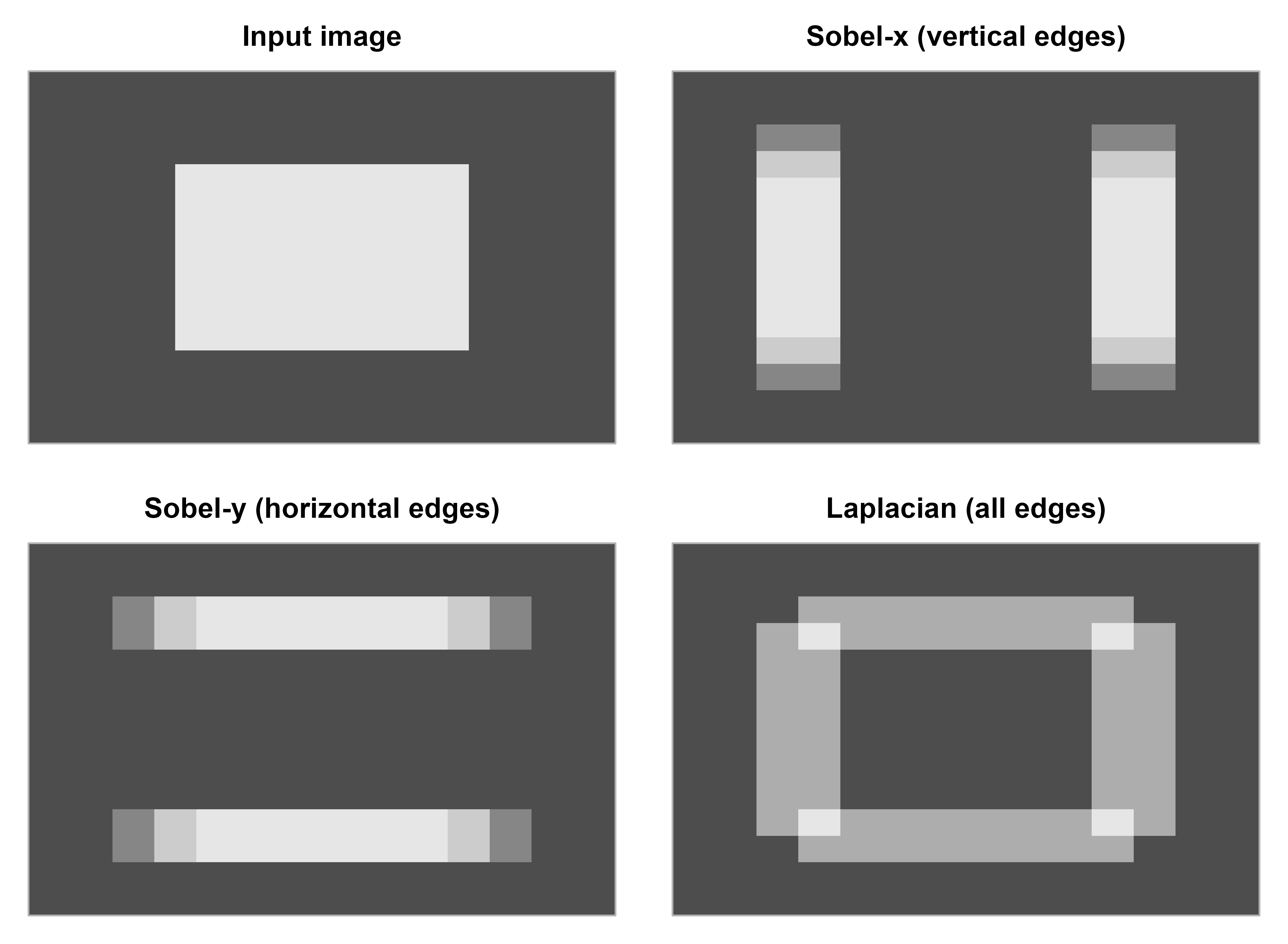
To make the operation concrete we implement Equation 36.2 in base R and apply real edge-detection kernels to a small synthetic image. The image is a grey square on a darker background, so it has crisp vertical and horizontal edges that the kernels should expose. Nothing here needs a deep learning library; convolution is just sliding-multiply-add.

Show code

# --- A tiny 2D convolution (cross-correlation), valid padding, stride 1 -------
conv2d <- function(img, kernel) {
  kh <- nrow(kernel); kw <- ncol(kernel)
  H  <- nrow(img);    W  <- ncol(img)
  Hout <- H - kh + 1                     # output-size formula, p = 0, s = 1
  Wout <- W - kw + 1
  out  <- matrix(0, Hout, Wout)
  for (i in seq_len(Hout)) {
    for (j in seq_len(Wout)) {
      patch     <- img[i:(i + kh - 1), j:(j + kw - 1)]
      out[i, j] <- sum(patch * kernel)   # multiply-add over the patch
    }
  }
  out
}

# --- Build a 16x16 image: a bright square on a dark background ----------------
set.seed(1)
img <- matrix(0.15, 16, 16)
img[5:12, 5:12] <- 0.85

# --- Classic 3x3 edge-detection kernels --------------------------------------
sobel_x <- matrix(c(-1, 0, 1,
                    -2, 0, 2,
                    -1, 0, 1), 3, 3, byrow = TRUE)   # vertical edges
sobel_y <- matrix(c(-1, -2, -1,
                     0,  0,  0,
                     1,  2,  1), 3, 3, byrow = TRUE)  # horizontal edges
laplace <- matrix(c( 0, -1,  0,
                    -1,  4, -1,
                     0, -1,  0), 3, 3, byrow = TRUE)  # all edges

edge_x <- conv2d(img, sobel_x)
edge_y <- conv2d(img, sobel_y)
edge_l <- conv2d(img, laplace)

# --- Verify the output-size formula (eq-cnn-outsize) --------------------------
cat(sprintf("Input %dx%d, 3x3 kernel, p=0, s=1  ->  output %dx%d\n",
            nrow(img), ncol(img), nrow(edge_x), ncol(edge_x)))
#> Input 16x16, 3x3 kernel, p=0, s=1  ->  output 14x14

# --- Show input and the three feature maps -----------------------------------
show_map <- function(m, title) {
  image(t(apply(m, 2, rev)), col = grey.colors(64),
        axes = FALSE, main = title)
  box(col = "grey70")
}
op <- par(mfrow = c(2, 2), mar = c(1, 1, 2.5, 1))
show_map(img,    "Input image")
show_map(abs(edge_x), "Sobel-x (vertical edges)")
show_map(abs(edge_y), "Sobel-y (horizontal edges)")
show_map(abs(edge_l), "Laplacian (all edges)")

Show code

par(op)

The size report confirms Equation 36.4: a $16 \times 16$ image convolved with a $3 \times 3$ kernel at stride $1$ with no padding yields a $14 \times 14$ feature map, exactly $H - k_h + 1$. The four panels (rendered above) make the operation visible. The input is a solid bright square. The Sobel-x map fires along the left and right sides of the square, where intensity changes horizontally (a vertical edge), and is dark everywhere the image is flat. The Sobel-y map fires along the top and bottom. The Laplacian responds to every edge at once. These are not learned weights; they are the hand-designed filters that inspired the very first conv layers, and a trained CNN discovers filters like these on its own in its earliest layer. To check the backward-pass result of Section 36.6 numerically, we confirm that the weight gradient of Equation 36.9 matches a finite-difference gradient.

Show code

# Forward: s = conv2d(x, w); loss = sum(delta * s) for a fixed upstream delta.
# Then dL/dw should equal conv2d(x, delta) by eq-cnn-dw.
set.seed(7)
x     <- matrix(rnorm(8 * 8), 8, 8)
w     <- matrix(rnorm(3 * 3), 3, 3)
s     <- conv2d(x, w)
delta <- matrix(rnorm(length(s)), nrow(s), ncol(s))   # upstream gradient

loss  <- function(w) sum(delta * conv2d(x, w))

grad_analytic <- conv2d(x, delta)                     # eq-cnn-dw

# Finite-difference gradient for comparison
grad_numeric <- matrix(0, 3, 3)
eps <- 1e-6
for (a in 1:3) for (b in 1:3) {
  wp <- w; wp[a, b] <- wp[a, b] + eps
  wm <- w; wm[a, b] <- wm[a, b] - eps
  grad_numeric[a, b] <- (loss(wp) - loss(wm)) / (2 * eps)
}

cat("Max abs difference (analytic vs numeric):",
    format(max(abs(grad_analytic - grad_numeric)), digits = 3), "\n")
#> Max abs difference (analytic vs numeric): 1.48e-09

The two gradients agree to within numerical-differentiation error, confirming the central claim of Section 36.6: the gradient of a convolution is itself a convolution. With the forward operation, the size formula, and the backward operation all verified on a few lines of base R, the machinery that a deep learning library scales to millions of parameters and GPU kernels is no longer a black box.

36.10 Summary

Convolutional networks replace the dense layer’s blind flattening with two structural priors that match grid data: locality (each unit sees a small patch) and weight sharing (one filter is reused everywhere). Those priors slash the parameter count by orders of magnitude (Equation 36.5 versus Equation 36.6), encode translation equivariance, and let depth build a hierarchy of features whose receptive fields grow with each layer. The forward pass is the sliding-multiply-add of Equation 36.2, sized by Equation 36.4; pooling adds cheap invariance and downsampling; and the backward pass (Equation 36.9, Equation 36.10) is again a convolution, which is why training is efficient. Where convolution’s local view falls short, attention (Chapter 38) takes over, and the unsupervised cousins of these ideas appear in the autoencoders of Chapter 41.

https://www.deeplearningbook.org/↩︎

# Convolutional Neural Networks {#sec-cnn} ```{r} #| include: false source("_common.R") ``` Show a photograph to the feedforward networks of @sec-neural-networks and the first thing they do is throw away everything that makes it a photograph. A dense layer flattens the image into one long vector, so the pixel at the top left and the pixel just below it become two unrelated coordinates, no closer in the model's eyes than two pixels at opposite corners. The grid is gone. Yet the grid is the whole point: in an image, meaning lives in local arrangements of nearby pixels (an edge, a corner, a patch of texture) and those arrangements mean the same thing wherever they appear. A cat in the top left of the frame is still a cat in the bottom right. A network that has to relearn "what an edge looks like" separately for every location is wasting both its parameters and your data. Convolutional neural networks (CNNs) are built around two ideas that put that lost structure back. The first is locality: a unit should look at a small neighborhood of the input, not all of it, because the features that matter are local. The second is weight sharing: the same small set of weights (a filter, or kernel) is slid across the entire image, so a feature detector learned in one place is reused everywhere. Together these turn a dense layer with millions of free parameters into a convolution with a few dozen, and they bake in an assumption (translation equivariance) that happens to be true for natural images. The result is the architecture that made deep learning famous on vision, and the same machinery extends to audio, text, and any data that lives on a grid. ::: {.callout-important title="Key idea"} A convolutional layer is a dense layer with two constraints imposed by hand: each output sees only a local patch of the input (locality), and every output reuses the same weights (sharing). These constraints are not a loss of generality. They encode the prior that useful features are local and appear anywhere, which is exactly the structure of grid data. ::: By the end of this chapter you will be able to write down the discrete convolution with stride and padding and compute the size of its output; count the parameters of a conv layer and see how few there are next to a dense layer; explain what pooling buys you and what it costs; read the canonical conv-pool-conv-pool-dense architecture and reason about how its receptive field grows with depth; and derive the backward pass, where you will see that the gradient of a convolution is itself a convolution. A runnable base-R demonstration applies real edge-detection kernels to a small image so that the convolution operation stops being abstract. CNNs sit alongside the autoencoders of @sec-autoencoders and the attention models of @sec-transformers as the third great family of deep architectures, and they share the gradient-based training machinery of @sec-neural-networks throughout. The treatment here follows the standard references, which are good next stops for more depth. - Deep Learning^[<https://www.deeplearningbook.org/>] [@Goodfellow-et-al-2016, Ch 9] - [@hastie2001a, Ch 11] - Deep Learning with R [@alma991043601650103276] ## Why Not Just Use a Dense Layer? It is worth being concrete about how badly a fully connected network scales on images, because the cost is what motivates everything that follows. Take a modest color image of $224 \times 224$ pixels with three channels (red, green, blue). Flattened, that is $224 \times 224 \times 3 = 150{,}528$ inputs. Connect it to a hidden layer of just $1000$ units and every one of those units needs a weight for every input, giving $150{,}528 \times 1000 \approx 1.5 \times 10^8$ weights in a single layer. That is more parameters in one layer than many full networks have, and we have not yet detected a single edge. With that many free parameters the model can memorize the training set effortlessly and generalizes poorly, exactly the overfitting risk discussed in @sec-neural-networks. The waste is not only in count, it is in structure. The dense layer treats the input as an unordered bag of numbers. It has no built-in notion that input $7{,}001$ sits directly below input $6{,}777$, so it cannot exploit the fact that adjacent pixels are correlated and that the same local pattern recurs across the image. Anything it learns about a feature in one corner it must learn again, from scratch and from separate examples, for every other corner. A convolutional layer fixes both problems at once: it connects each output to a small local patch (cutting the connection count), and it forces every output to share one filter (cutting the parameter count to the size of that single filter, independent of image size). ## The Convolution Operation The plain-language version is simple. Take a small grid of numbers, the kernel. Slide it across the image. At each position, multiply the kernel against the patch of image underneath it, add up the products, and write that single number into the output. Sweep over every position and the numbers you wrote out form a new image, called a feature map. A kernel tuned to respond to vertical edges lights up wherever the image has a vertical edge. That sliding-multiply-add is the whole operation. ### One dimension first Start in one dimension, where the bookkeeping is lightest. Let the input be a signal $x[0], x[1], \dots, x[n-1]$ and the kernel be $w[0], \dots, w[k-1]$. The operation a CNN actually computes (called cross-correlation, though the field universally calls it convolution) places the output at position $i$ as $$ s[i] = \sum_{a=0}^{k-1} x[i+a]\, w[a]. $$ {#eq-cnn-conv1d} Each output is a weighted sum of $k$ consecutive inputs, using the same weights $w$ at every position $i$. That single reuse of $w$ is weight sharing, and the fact that the sum runs only over $k$ neighbors (not all $n$ inputs) is locality. ::: {.callout-note title="Convolution versus cross-correlation"} The mathematician's convolution flips the kernel: $(x * w)[i] = \sum_a x[i-a]\, w[a]$. @eq-cnn-conv1d does not flip it. The two differ only by reversing the kernel, and since the kernel weights are learned, the network can absorb the flip into the weights it chooses. The distinction is therefore irrelevant to a CNN, and the deep learning literature uses "convolution" for the unflipped @eq-cnn-conv1d throughout. We follow that convention. ::: ### Two dimensions For an image $X$ of size $H \times W$ and a kernel $K$ of size $k_h \times k_w$, the two-dimensional version sums over a small rectangle: $$ S[i,j] = \sum_{a=0}^{k_h-1} \sum_{b=0}^{k_w-1} X[i+a,\; j+b]\; K[a,b]. $$ {#eq-cnn-conv2d} Real images have multiple input channels (three for RGB, or many more for the feature maps produced by an earlier layer). A single filter then has a kernel for every input channel, and the layer learns many filters, each producing one output channel. Writing $C_{\text{in}}$ for the number of input channels and indexing the output channel by $o$, the full layer computes $$ S_o[i,j] = b_o + \sum_{c=1}^{C_{\text{in}}}\sum_{a=0}^{k_h-1}\sum_{b=0}^{k_w-1} X_c[i+a,\; j+b]\; K_{o,c}[a,b], $$ {#eq-cnn-conv-full} where $b_o$ is a per-filter bias and $K_{o,c}$ is the slice of filter $o$ that acts on input channel $c$. A nonlinearity (typically the ReLU of @sec-neural-networks) is then applied elementwise to each $S_o$. The key structural fact is that the spatial indices $a,b$ range only over the small kernel, while the sum over channels $c$ is dense: a filter looks at a small spatial patch but all of the channels in it. ### Stride and padding Two knobs control how the kernel sweeps the image. Stride $s$ is how far the kernel jumps between positions. With $s=1$ it moves one pixel at a time and the output is nearly as large as the input. With $s=2$ it skips every other position, halving the output's height and width and cheaply downsampling the feature map. Padding $p$ adds a border of (usually zero) pixels around the input before convolving. Without padding the kernel cannot be centered on the edge pixels, so the output shrinks and border information is undersampled. Adding $p$ rows and columns of zeros on each side lets the output keep the input's size ("same" padding) and treats the borders evenly. With these, the output height is $$ H_{\text{out}} = \left\lfloor \frac{H + 2p - k_h}{s} \right\rfloor + 1, $$ {#eq-cnn-outsize} and $W_{\text{out}}$ is given by the identical formula in the width direction. Two sanity checks make this memorable. With no padding and unit stride ($p=0,\,s=1$) it gives $H_{\text{out}} = H - k_h + 1$: a $k_h$-tall kernel loses $k_h - 1$ rows because it cannot hang off the edge. To preserve the size with $s=1$, set $p = (k_h - 1)/2$, which is why odd kernel sizes like $3 \times 3$ and $5 \times 5$ are universal (they give an integer pad). ::: {.callout-tip title="A quick worked size"} A $32 \times 32$ input, a $5 \times 5$ kernel, stride $1$, no padding gives $\lfloor (32 + 0 - 5)/1 \rfloor + 1 = 28$, a $28 \times 28$ output. Switch to stride $2$ and you get $\lfloor 27/2 \rfloor + 1 = 14$, halving each dimension. Add padding $p=2$ at stride $1$ and you get $\lfloor (32 + 4 - 5)/1 \rfloor + 1 = 32$, the original size preserved. ::: ## Counting Parameters The payoff of weight sharing shows up the moment you count parameters, so it is worth doing carefully. A convolutional layer with $C_{\text{out}}$ filters, each of spatial size $k_h \times k_w$ and acting on $C_{\text{in}}$ input channels, has $$ \#\text{params}_{\text{conv}} = C_{\text{out}}\,\bigl(C_{\text{in}}\, k_h\, k_w + 1\bigr), $$ {#eq-cnn-params} where the $+1$ is the bias per filter. The striking feature of @eq-cnn-params is what it does not contain: the spatial size of the image, $H$ and $W$. A filter that scans a tiny image and one that scans a huge image cost the same, because the same kernel weights are reused at every position. Contrast a dense layer mapping the same input to the same number of outputs. If the input is $H \times W \times C_{\text{in}}$ and the output is $H_{\text{out}} \times W_{\text{out}} \times C_{\text{out}}$ values, a fully connected layer needs a separate weight for every (input, output) pair: $$ \#\text{params}_{\text{dense}} = (H\,W\,C_{\text{in}})\,(H_{\text{out}}\,W_{\text{out}}\,C_{\text{out}}) + H_{\text{out}}\,W_{\text{out}}\,C_{\text{out}}. $$ {#eq-cnn-params-dense} Put numbers in. A $28 \times 28$ single-channel input, a layer producing $32$ feature maps with $3 \times 3$ filters and "same" padding so the output is $28 \times 28 \times 32$. The conv layer costs $32 \times (1 \times 3 \times 3 + 1) = 320$ parameters. A dense layer producing the same $28 \times 28 \times 32 = 25{,}088$ outputs from the $784$ inputs costs $784 \times 25{,}088 + 25{,}088 \approx 1.97 \times 10^7$ parameters. The convolution is roughly sixty thousand times smaller and, because of weight sharing, it generalizes from far less data. ::: {.callout-note title="Equivariance, the prior you are buying"} Weight sharing makes convolution translation equivariant: shift the input and the feature map shifts by the same amount, $\text{conv}(\text{shift}(x)) = \text{shift}(\text{conv}(x))$. The network does not need to see an object in every position to recognize it in every position. This is the inductive bias that pays for the constraint, and it is exactly right for images, where content can appear anywhere. ::: ## Pooling After a convolution we usually want to summarize each small neighborhood and shrink the feature map. Pooling does this with no parameters at all. A pooling window of size $r \times r$ slides over the feature map (typically with stride $r$, so windows do not overlap) and replaces each window with a single number. Max pooling takes the largest value in the window, $$ P[i,j] = \max_{0 \le a,b < r} S[\,i\,r + a,\; j\,r + b\,], $$ {#eq-cnn-maxpool} and average pooling takes the mean instead. Max pooling reports whether a feature was detected anywhere in the window, discarding its exact position, which gives a small amount of translation invariance: jiggle the input by less than the window and the pooled output is unchanged. It also halves the spatial dimensions (with $r=2$), cutting the computation of every layer that follows. Pooling has a cost worth naming. By throwing away position it can hurt tasks where precise location matters, such as segmentation, and modern architectures often replace it with strided convolutions (which downsample while still learning weights). For classification, where you ultimately want "is there a cat, anywhere," the invariance pooling provides is usually a feature, not a bug. ## The Canonical Architecture and the Receptive Field Stack the pieces and a classic image classifier emerges: convolution, nonlinearity, pooling, repeated a few times, then a flatten and one or two dense layers to a softmax over classes. The pattern is conv-pool-conv-pool-dense, and @fig-cnn-architecture sketches it. ```{mermaid} %%| label: fig-cnn-architecture %%| fig-cap: "The canonical convolutional classifier. Convolution and pooling blocks build up spatial features while shrinking resolution; a flatten and dense head turns those features into class scores." graph LR IN["Input image HxWxC"] --> C1["Conv + ReLU (local features)"] C1 --> P1["Pool (downsample)"] P1 --> C2["Conv + ReLU (richer features)"] C2 --> P2["Pool (downsample)"] P2 --> FL["Flatten"] FL --> D1["Dense + ReLU"] D1 --> OUT["Softmax (class scores)"] ``` The reason depth helps is the receptive field: the region of the original input that a given unit can "see." A unit in the first conv layer with a $k \times k$ kernel sees a $k \times k$ patch. A unit in the second conv layer sees a $k \times k$ patch of the first layer's output, and each of those came from a $k \times k$ patch of the input, so the second-layer unit's receptive field is larger. Pooling and stride accelerate this growth because each downsampling step multiplies the input area covered per step. For a stack of conv layers with kernel size $k$, stride $1$, and no pooling, the receptive field after $L$ layers is $$ R_L = 1 + L\,(k-1), $$ {#eq-cnn-rf} growing linearly with depth. Insert pooling or strided layers and the growth becomes multiplicative, which is how a network of $3 \times 3$ kernels can end up with units that respond to whole objects. This is the hierarchy at work: early layers detect edges and blobs, middle layers assemble them into textures and parts, deep layers represent whole objects, with each level reusing the level below. It is the same compositional story as the deep feedforward networks of @sec-neural-networks, specialized to space. ## Backpropagation Through a Convolution {#sec-cnn-backprop} Training a CNN uses the same gradient descent as any other network (@sec-neural-networks); the only new work is differentiating the convolution. The clean result, and the reason convolutions are efficient to train, is that every gradient in a conv layer is itself a convolution. We derive it in one dimension using @eq-cnn-conv1d; the two-dimensional case is identical with an extra index. Let the loss be $\mathcal{L}$ and let the gradient arriving at the layer output be $\delta[i] = \partial \mathcal{L} / \partial s[i]$, supplied by backprop from above. We need two things: the gradient with respect to the kernel weights $w$ (to update them) and the gradient with respect to the input $x$ (to pass further back). Start with the weights. Because $w[a]$ is shared across every output position, it appears in $s[i]$ for every $i$, so the chain rule sums its contributions over all positions: $$ \frac{\partial \mathcal{L}}{\partial w[a]} = \sum_i \frac{\partial \mathcal{L}}{\partial s[i]} \frac{\partial s[i]}{\partial w[a]} = \sum_i \delta[i]\, x[i+a]. $$ {#eq-cnn-dw} Read @eq-cnn-dw as a function of $a$: it is the cross-correlation of the input $x$ with the upstream gradient $\delta$. The weight gradient is a convolution of the forward input against the backward signal. (The sum over all positions is exactly where weight sharing reappears in the backward pass, accumulating one update for the single shared kernel.) Now the input. The pixel $x[m]$ enters $s[i]$ only when $i + a = m$ for some valid $a$, that is when $a = m - i$. From @eq-cnn-conv1d, $\partial s[i]/\partial x[m] = w[m-i]$ whenever $0 \le m - i < k$ and zero otherwise. The chain rule gives $$ \frac{\partial \mathcal{L}}{\partial x[m]} = \sum_i \delta[i]\, \frac{\partial s[i]}{\partial x[m]} = \sum_i \delta[i]\, w[m-i]. $$ {#eq-cnn-dx} The right side of @eq-cnn-dx is a convolution (with the flip, in the strict mathematical sense) of the upstream gradient $\delta$ with the kernel $w$. Equivalently it is the cross-correlation of $\delta$ with the kernel reversed, often called the "full" or transposed convolution. Either way, the backward pass through a conv layer is another conv layer, so it runs in the same time as the forward pass and reuses the same highly optimized routines. This is the structural reason CNNs train efficiently. ::: {.callout-note title="The three convolutions of a conv layer"} A convolutional layer involves a convolution in each of its three roles. The forward pass (@eq-cnn-conv2d) convolves input with kernel. The weight gradient (@eq-cnn-dw) convolves input with the upstream gradient. The input gradient (@eq-cnn-dx) convolves the upstream gradient with the flipped kernel. One operation, three uses. ::: ## Complexity, Assumptions, and Failure Modes The computational cost of a conv layer is the number of output positions times the work per position. For an output of size $H_{\text{out}} \times W_{\text{out}}$ with $C_{\text{out}}$ filters, each summing over $C_{\text{in}} k_h k_w$ terms, the forward cost is $$ O\bigl(H_{\text{out}}\, W_{\text{out}}\, C_{\text{out}}\, C_{\text{in}}\, k_h\, k_w\bigr). $$ {#eq-cnn-flops} Unlike the parameter count of @eq-cnn-params, the compute does scale with image size through $H_{\text{out}} W_{\text{out}}$, because the same small kernel is applied at every one of those positions. The practical consequence is that CNNs are parameter-light but compute-heavy, which is why they ride on GPUs. The assumptions that make convolution work are equally worth stating, because they identify when it fails. - Stationarity and locality. Convolution assumes the same local features are useful everywhere and that what matters is local. On data where this holds (natural images, audio, time series) it is a powerful prior. On data where position carries fixed meaning (a spreadsheet column, where column $3$ is always "age") weight sharing is wrong and a dense or tabular model is better. - Limited global context. A single conv layer sees only its kernel; long-range relationships must be assembled through depth, which can be inefficient. This is precisely the gap that the attention mechanism of @sec-transformers fills, and modern vision increasingly blends or replaces convolution with attention. - Sensitivity to large transformations. Equivariance buys robustness to small translations only. Large rotations, scale changes, and adversarial perturbations are not handled for free and require data augmentation or specialized layers. CNNs are also famously vulnerable to imperceptible adversarial noise, a failure mode they share with deep networks generally. - Data hunger and opacity. Despite the parameter savings, competitive CNNs still need large labeled datasets, and like the rest of the deep learning family (@sec-neural-networks) they are hard to interpret, motivating the tools of @sec-interpretable-machine-learning. ## Practical How-To A few rules of thumb cover most of what you need to build a working CNN. - Prefer small kernels and depth. Two stacked $3 \times 3$ convolutions have the same receptive field as one $5 \times 5$ but fewer parameters and an extra nonlinearity, so the field standardized on small kernels. - Grow channels as you shrink space. As pooling and stride reduce $H$ and $W$, increase $C_{\text{out}}$ (for example $32 \to 64 \to 128$) so the representation keeps capacity while resolution drops. - Normalize and augment. Batch normalization stabilizes and speeds training; data augmentation (random crops, flips, small rotations) manufactures the translation and scale variation that equivariance alone does not cover. - Use "same" padding with odd kernels so spatial sizes are predictable, and reach for transfer learning (start from a network pretrained on a large dataset) whenever your own labeled data is limited, a pattern that dominates applied vision. The Keras code below shows the canonical classifier end to end. It is shown but not executed here, since it requires a GPU-backed deep learning stack. ```{r} #| eval: false library(keras) model <- keras_model_sequential() |> layer_conv_2d(filters = 32, kernel_size = c(3, 3), activation = "relu", padding = "same", input_shape = c(28, 28, 1)) |> layer_max_pooling_2d(pool_size = c(2, 2)) |> layer_conv_2d(filters = 64, kernel_size = c(3, 3), activation = "relu", padding = "same") |> layer_max_pooling_2d(pool_size = c(2, 2)) |> layer_flatten() |> layer_dense(units = 128, activation = "relu") |> layer_dropout(rate = 0.5) |> layer_dense(units = 10, activation = "softmax") model |> compile( optimizer = "adam", loss = "sparse_categorical_crossentropy", metrics = "accuracy" ) # x_train: array of shape (n, 28, 28, 1); y_train: integer labels 0..9 model |> fit(x_train, y_train, epochs = 10, batch_size = 128, validation_split = 0.1) ``` ## A Runnable Demonstration: Convolution by Hand To make the operation concrete we implement @eq-cnn-conv2d in base R and apply real edge-detection kernels to a small synthetic image. The image is a grey square on a darker background, so it has crisp vertical and horizontal edges that the kernels should expose. Nothing here needs a deep learning library; convolution is just sliding-multiply-add. ```{r} #| label: cnn-conv-demo #| fig-width: 7.5 #| fig-height: 5.5 #| out-width: "95%" # --- A tiny 2D convolution (cross-correlation), valid padding, stride 1 ------- conv2d <- function(img, kernel) { kh <- nrow(kernel); kw <- ncol(kernel) H <- nrow(img); W <- ncol(img) Hout <- H - kh + 1 # output-size formula, p = 0, s = 1 Wout <- W - kw + 1 out <- matrix(0, Hout, Wout) for (i in seq_len(Hout)) { for (j in seq_len(Wout)) { patch <- img[i:(i + kh - 1), j:(j + kw - 1)] out[i, j] <- sum(patch * kernel) # multiply-add over the patch } } out } # --- Build a 16x16 image: a bright square on a dark background ---------------- set.seed(1) img <- matrix(0.15, 16, 16) img[5:12, 5:12] <- 0.85 # --- Classic 3x3 edge-detection kernels -------------------------------------- sobel_x <- matrix(c(-1, 0, 1, -2, 0, 2, -1, 0, 1), 3, 3, byrow = TRUE) # vertical edges sobel_y <- matrix(c(-1, -2, -1, 0, 0, 0, 1, 2, 1), 3, 3, byrow = TRUE) # horizontal edges laplace <- matrix(c( 0, -1, 0, -1, 4, -1, 0, -1, 0), 3, 3, byrow = TRUE) # all edges edge_x <- conv2d(img, sobel_x) edge_y <- conv2d(img, sobel_y) edge_l <- conv2d(img, laplace) # --- Verify the output-size formula (eq-cnn-outsize) -------------------------- cat(sprintf("Input %dx%d, 3x3 kernel, p=0, s=1 -> output %dx%d\n", nrow(img), ncol(img), nrow(edge_x), ncol(edge_x))) # --- Show input and the three feature maps ----------------------------------- show_map <- function(m, title) { image(t(apply(m, 2, rev)), col = grey.colors(64), axes = FALSE, main = title) box(col = "grey70") } op <- par(mfrow = c(2, 2), mar = c(1, 1, 2.5, 1)) show_map(img, "Input image") show_map(abs(edge_x), "Sobel-x (vertical edges)") show_map(abs(edge_y), "Sobel-y (horizontal edges)") show_map(abs(edge_l), "Laplacian (all edges)") par(op) ``` The size report confirms @eq-cnn-outsize: a $16 \times 16$ image convolved with a $3 \times 3$ kernel at stride $1$ with no padding yields a $14 \times 14$ feature map, exactly $H - k_h + 1$. The four panels (rendered above) make the operation visible. The input is a solid bright square. The Sobel-x map fires along the left and right sides of the square, where intensity changes horizontally (a vertical edge), and is dark everywhere the image is flat. The Sobel-y map fires along the top and bottom. The Laplacian responds to every edge at once. These are not learned weights; they are the hand-designed filters that inspired the very first conv layers, and a trained CNN discovers filters like these on its own in its earliest layer. To check the backward-pass result of @sec-cnn-backprop numerically, we confirm that the weight gradient of @eq-cnn-dw matches a finite-difference gradient. ```{r} #| label: cnn-backprop-check # Forward: s = conv2d(x, w); loss = sum(delta * s) for a fixed upstream delta. # Then dL/dw should equal conv2d(x, delta) by eq-cnn-dw. set.seed(7) x <- matrix(rnorm(8 * 8), 8, 8) w <- matrix(rnorm(3 * 3), 3, 3) s <- conv2d(x, w) delta <- matrix(rnorm(length(s)), nrow(s), ncol(s)) # upstream gradient loss <- function(w) sum(delta * conv2d(x, w)) grad_analytic <- conv2d(x, delta) # eq-cnn-dw # Finite-difference gradient for comparison grad_numeric <- matrix(0, 3, 3) eps <- 1e-6 for (a in 1:3) for (b in 1:3) { wp <- w; wp[a, b] <- wp[a, b] + eps wm <- w; wm[a, b] <- wm[a, b] - eps grad_numeric[a, b] <- (loss(wp) - loss(wm)) / (2 * eps) } cat("Max abs difference (analytic vs numeric):", format(max(abs(grad_analytic - grad_numeric)), digits = 3), "\n") ``` The two gradients agree to within numerical-differentiation error, confirming the central claim of @sec-cnn-backprop: the gradient of a convolution is itself a convolution. With the forward operation, the size formula, and the backward operation all verified on a few lines of base R, the machinery that a deep learning library scales to millions of parameters and GPU kernels is no longer a black box. ## Summary Convolutional networks replace the dense layer's blind flattening with two structural priors that match grid data: locality (each unit sees a small patch) and weight sharing (one filter is reused everywhere). Those priors slash the parameter count by orders of magnitude (@eq-cnn-params versus @eq-cnn-params-dense), encode translation equivariance, and let depth build a hierarchy of features whose receptive fields grow with each layer. The forward pass is the sliding-multiply-add of @eq-cnn-conv2d, sized by @eq-cnn-outsize; pooling adds cheap invariance and downsampling; and the backward pass (@eq-cnn-dw, @eq-cnn-dx) is again a convolution, which is why training is efficient. Where convolution's local view falls short, attention (@sec-transformers) takes over, and the unsupervised cousins of these ideas appear in the autoencoders of @sec-autoencoders.