Advanced Data Analysis

Nguyen, Mike

21 Quantile Regression

Ordinary least squares answers one question very well: given the predictors, what is the average value of the outcome? The fitted line traces the conditional mean, $E(y|x)$, and a single slope summarizes how that average moves as $x$ moves. That is often exactly what we want. But the average can hide a great deal. Two groups of patients might have the same mean recovery time while one group has a long, heavy upper tail of slow recoverers that a clinic cares about most. A pay-equity study might find no difference in mean salary across groups while the gap is large at the top of the pay scale and absent at the bottom. In both cases the interesting action is in the shape of the distribution, not its center, and the mean alone cannot see it.

Quantile regression widens the lens. Instead of modeling only the mean, it models any quantile (any percentile) of the outcome distribution as a function of the predictors. We can ask how the 10th percentile of $y$ responds to $x$, how the median responds, how the 90th percentile responds, and compare those answers. When the relationship is the same at every quantile, quantile regression simply reproduces the OLS story. When it differs, quantile regression reveals structure (changing spread, skewness, effects that grow in the tails) that a mean model averages away.

Key idea

OLS estimates the conditional mean $E(y|x)$. Quantile regression estimates a conditional quantile $Q_q(y|x)$, the value below which a fraction $q$ of the outcome falls at each setting of $x$. Sweeping $q$ from near 0 to near 1 gives a family of fits that describes the whole conditional distribution, not just its center.

In this chapter you will learn what a conditional quantile is and why we might prefer it to the mean, how the model is fit by minimizing an asymmetric absolute-error loss (the “tilted” or “check” loss), how to read the resulting coefficients, and how to estimate and visualize quantile fits in R with the quantreg package. The classic reference for the method is Koenker (2005); for an accessible academic review see Yu, Lu, and Stander (2003).

The most familiar special case is the median. When $q = 0.5$, quantile regression becomes median regression, also called least-absolute-deviations (LAD) regression, which chooses the line minimizing the sum of absolute residuals $\sum_{i}|e_i|$ rather than the sum of squared residuals. Because absolute errors do not square large deviations, the median fit is far less sensitive to a few extreme points than the mean fit is.

Intuition

OLS minimizes squared errors, so a single far-away point can drag the whole line toward it. LAD (median) regression minimizes absolute errors, so an outlier counts in proportion to its distance rather than its distance squared. That is the same reason the median of a list of numbers barely moves when you replace its largest value with something ten times larger, while the mean lurches.

21.1 Why and when to use it

It helps to be explicit about what quantile regression buys you and what it costs, before getting into the mechanics.

The main attractions are these. Quantile regression is more robust to outliers than OLS, because it rests on absolute rather than squared loss. It gives a fuller picture of the data, describing how the entire conditional distribution shifts with the predictors rather than reporting a single average effect, which is especially valuable when the outcome is skewed or has a bimodal or multimodal distribution (several humps with several modes) that a mean would misrepresent.¹ It makes no parametric assumption about the error distribution: we do not have to claim the errors are normal or anything else, which connects it to the nonparametric view of the outcome’s full distribution taken up in the density estimation chapter (Chapter 32). And it has a clean equivariance property that OLS lacks: quantiles are preserved under monotone transformations, so the $q$th quantile of $g(y)$ is $g$ applied to the $q$th quantile of $y$ for any increasing $g$. OLS does not share this, since in general $E(g(y)) \neq g(E(y))$.²

The estimated coefficients also behave well for inference: under standard conditions the quantile-regression estimator $\hat\beta$ is asymptotically normally distributed, which lets us attach standard errors and confidence intervals.

When to use this

Reach for quantile regression when you care about more than the average, when the outcome is skewed or heavy-tailed, when effects plausibly differ across the distribution (small at the median, large in the tail), or when outliers make an OLS mean untrustworthy. (When the outliers themselves are the object of interest rather than a nuisance, see the anomaly and outlier detection chapter, Chapter 87.)

There is one practical limitation worth flagging. Quantile regression works best when the outcome is continuous. If the dependent variable has many tied values or piles of zeros (so that whole ranges of the distribution sit at a single number), individual quantiles become poorly identified and the method is less informative.

Warning

Avoid quantile regression when the outcome is discrete with heavy ties or has a large mass of zeros (for example, count or censored data with many zeros). The quantiles you are trying to estimate may not be uniquely defined there.

21.2 The model and its loss function

The model looks like a linear regression, but the coefficient vector now depends on the quantile $q$ we have chosen to target:

\[ y_i = x_i'\beta_q + e_i \]

Everything hinges on how we measure the error. Write the residual as $e(x) = y - \hat{y}(x)$, and let $L(e(x)) = L(y - \hat{y}(x))$ be the loss we pay for that error. OLS uses squared loss; here we start from absolute loss. If $L(e) = |e|$, the absolute-error loss function, then $\hat\beta$ is found by minimizing $\sum_i |y_i - x_i'\beta|$, which is exactly median (LAD) regression.

To target a quantile other than the median, we tilt this absolute loss so that under-prediction and over-prediction are penalized differently. The objective function for quantile $q$ is

\[ Q(\beta_q)=\sum_{i:y_i \ge x_i'\beta}^{N} q|y_i - x_i'\beta_q| + \sum_{i:y_i < x_i'\beta}^{N} (1-q)|y_i-x_i'\beta_q| \]

where $0 < q < 1$. The first sum collects the points lying above the fitted line (where we under-predicted) and weights their absolute errors by $q$; the second sum collects the points below the line (where we over-predicted) and weights theirs by $1 - q$.

Intuition

This asymmetric weighting is what pins the fit to a particular quantile. Suppose $q = 0.9$. Then under-prediction costs $0.9$ per unit of error while over-prediction costs only $0.1$. To keep the total small, the line is pushed up until about 90% of the points sit below it, which is precisely the definition of the 90th percentile. Set $q = 0.5$ and the two weights are equal, the loss is symmetric, and we recover median regression.

Because $|e|$ has a kink at zero, the objective is not differentiable, so there is no closed-form normal-equation solution as in OLS. Instead the problem is solved as a linear program, classically with the simplex method, and standard errors are commonly obtained by the bootstrap rather than from a formula.³

21.2.1 Precise formulation: the check loss

To reason about the estimator we need notation that is both compact and exact. Define the check function (also called the pinball or tilted absolute loss) at level $q \in (0,1)$,

\[ \rho_q(u) = u\bigl(q - \mathbb{1}\{u < 0\}\bigr) = \begin{cases} q\,u, & u \ge 0,\\[2pt] (q-1)\,u, & u < 0, \end{cases} \tag{21.1}\]

where $\mathbb{1}\{\cdot\}$ is the indicator. Both branches are nonnegative: for $u \ge 0$ the loss is $qu \ge 0$, and for $u < 0$ the loss is $(q-1)u = (1-q)|u| \ge 0$. The objective $Q(\beta_q)$ written out term by term above is exactly $\sum_{i=1}^N \rho_q\!\left(y_i - x_i'\beta_q\right)$, with the two summation ranges corresponding to the two branches of Equation 21.1. The quantile-regression estimator is

\[ \hat\beta_q = \arg\min_{\beta \in \mathbb{R}^p} \sum_{i=1}^N \rho_q\!\left(y_i - x_i'\beta\right). \tag{21.2}\]

The conditional quantile being estimated is defined through the conditional distribution function $F_{y|x}$: the $q$th conditional quantile is

\[ Q_q(y \mid x) = \inf\{\, t : F_{y\mid x}(t) \ge q \,\} = F_{y\mid x}^{-1}(q), \tag{21.3}\]

and the linear model asserts $Q_q(y\mid x) = x'\beta_q$. Crucially this is a model of the quantile, not of the mean plus an additive error of fixed shape: nothing requires the errors $e_i = y_i - x_i'\beta_q$ to be identically distributed or symmetric, only that the $q$th conditional quantile of $e_i$ given $x_i$ be zero, that is $\Pr(e_i \le 0 \mid x_i) = q$. This single restriction is the entire stochastic assumption.

21.2.2 Why minimizing the check loss returns a quantile

The asymmetric weighting story is correct but informal. Here is the derivation that makes it exact, first for the unconditional case (an intercept-only model), which already contains the whole idea.

Let $Y$ be a random variable with distribution function $F$ and consider choosing a single number $t$ to minimize the expected check loss,

\[ R(t) = \mathbb{E}\,\rho_q(Y - t) = q\!\int_{t}^{\infty}\!(y-t)\,dF(y) \;+\; (1-q)\!\int_{-\infty}^{t}\!(t-y)\,dF(y). \]

Differentiate with respect to $t$. Using Leibniz’s rule (the integrand vanishes at the moving endpoint $y=t$, so only the explicit $t$ inside the integrands contributes),

\[ R'(t) = -q\!\int_{t}^{\infty}\! dF(y) + (1-q)\!\int_{-\infty}^{t}\! dF(y) = -q\bigl(1 - F(t)\bigr) + (1-q)F(t). \]

Setting $R'(t)=0$ and solving,

\[ -q + qF(t) + F(t) - qF(t) = 0 \;\Longrightarrow\; F(t) = q, \]

so the minimizer satisfies $F(t) = q$, that is $t = F^{-1}(q)$, the $q$th quantile. The second derivative is $R''(t) = f(t) \ge 0$ wherever the density exists, confirming a minimum, and convexity of $\rho_q$ guarantees it is the global one. Setting $q = \tfrac12$ recovers $F(t) = \tfrac12$, the median, and the symmetric absolute loss. This is the population analogue of the fact that the sample check-loss minimizer puts a fraction $q$ of points below the fit.

For the regression case the same calculation runs on the subgradient. Because $\rho_q$ is convex but kinked at $0$, $\hat\beta_q$ is characterized by the condition that the zero vector lies in the subdifferential of Equation 21.2. Away from the kink, $\rho_q'(u) = q - \mathbb{1}\{u<0\} = \psi_q(u)$, and the optimality (normal-equation analogue) condition is

\[ \sum_{i=1}^N x_i\,\psi_q\!\left(y_i - x_i'\hat\beta_q\right) = 0, \qquad \psi_q(u) = q - \mathbb{1}\{u < 0\}, \tag{21.4}\]

with the residuals that are exactly zero contributing subgradient values in $[\,q-1,\,q\,]$ chosen to balance the sum. Compare this to the OLS normal equation $\sum_i x_i(y_i - x_i'\hat\beta) = 0$: quantile regression replaces the raw residual by the bounded, sign-and-tilt score $\psi_q$, which is why a far-away point exerts influence only through its sign, not its magnitude. That bounded score is the precise source of the robustness claimed earlier.

A useful corollary of Equation 21.4: take the row corresponding to the intercept, where $x_{i1}=1$. Then $\sum_i \psi_q(\hat e_i) = 0$, i.e. $q N$ equals the number of strictly negative residuals plus a fractional contribution from the exact zeros. In general position a fitted quantile plane interpolates exactly $p$ observations (the residuals at those points are zero), and a fraction approximately $q$ of the remaining residuals are negative. This is the regression generalization of “the median has half the data on each side.”

Note

“Not differentiable” sounds like trouble but is not. The loss is still convex, so the optimization is reliable; we just use linear-programming machinery instead of calculus. The quantreg package handles all of this for you.

21.2.3 Interpreting the coefficients

The payoff of all this is an interpretation that parallels OLS but applies at a chosen point of the distribution. For the $j$th predictor $x_j$, the coefficient is the marginal effect on the $q$th conditional quantile:

\[ \frac{\partial Q_q(y|x)}{\partial x_j} = \beta_{qj} \]

In words: at the $q$th quantile of $y$, a one-unit increase in $x_j$ is associated with a $\beta_{qj}$-unit change in $y$, holding the other predictors fixed. The reading is the same sentence you would write for an OLS slope, with one addition: it applies at that quantile rather than to the average.

Key idea

A single OLS regression gives you one slope per predictor. Quantile regression run across many values of $q$ gives you a curve of slopes, one per quantile, showing whether a predictor matters more at the bottom, the middle, or the top of the outcome distribution.

21.2.4 The linear-programming representation

The claim that Equation 21.2 “is a linear program” can be made literal, which both explains how rq computes the fit and exposes the dual that drives inference. Split each residual into its positive and negative parts, $u_i = (y_i - x_i'\beta)^+ \ge 0$ and $v_i = (y_i - x_i'\beta)^- \ge 0$, so that $y_i - x_i'\beta = u_i - v_i$ and $\rho_q(y_i - x_i'\beta) = q\,u_i + (1-q)\,v_i$. The estimation problem becomes the linear program

\[ \min_{\beta,\,u,\,v}\; q\,\mathbf{1}'u + (1-q)\,\mathbf{1}'v \quad\text{s.t.}\quad X\beta + u - v = y,\;\; u \ge 0,\;\; v \ge 0, \tag{21.5}\]

with $\beta$ free. This has $N$ equality constraints and $2N + p$ variables; its solution is a basic feasible point at which $p$ residuals are zero, recovering the interpolation property noted above. The classical solver is a simplex method specialized to this structure (Barrodale to Roberts, used by rq(method="br"), exact and excellent for small to moderate $N$); for large $N$ an interior-point method with preprocessing (method="pfn" or the Frisch to Newton variant) scales much better. The dual variables $a_i$ of Equation 21.5 lie in $[q-1,\,q]$ and are the “regression rank scores” used by one family of inference procedures.

Note

The cost of a single quantile fit is comparable to that of a least-squares fit for moderate sizes: $O(N p^2)$-ish for the linear algebra, with the simplex overhead. Fitting a whole grid of quantiles is cheap because rq can warm-start each fit from the neighboring one (the entire solution path in $q$ is itself piecewise constant in $\beta$, and rq(tau=-1) returns it exactly via parametric programming).

21.2.5 Asymptotic distribution and inference

The estimator is consistent and asymptotically normal under mild conditions (continuous conditional density positive at the quantile, finite design moments). Writing $\beta_q$ for the truth and $f_{y\mid x}$ for the conditional density of $y$, the standard result (Koenker (2005)) is

\[ \sqrt{N}\,\bigl(\hat\beta_q - \beta_q\bigr) \;\xrightarrow{d}\; \mathcal{N}\!\left(0,\; \tau\,(1-\tau)\,D_1^{-1} D_0\, D_1^{-1}\right), \tag{21.6}\]

with $\tau = q$, $D_0 = \mathbb{E}\!\left[x x'\right]$ and the sparsity-weighted matrix

\[ D_1 = \mathbb{E}\!\left[\,f_{y\mid x}\!\bigl(x'\beta_q \mid x\bigr)\, x x'\,\right]. \]

The sandwich has the same algebraic shape as in M-estimation: the meat $\tau(1-\tau)D_0$ is the variance of the score $\psi_q$ (note $\operatorname{Var}\psi_q = q(1-q)$), and the bread $D_1^{-1}$ is the inverse expected Jacobian. The density factor $f_{y\mid x}$ inside $D_1$ is the catch: precision degrades where the conditional density is low, so estimates in the far tails (small or large $q$) are noisier, and the reciprocal density $1/f$ is called the sparsity function. In the special case of i.i.d. errors with density $f$, $D_1 = f(F^{-1}(q))\,D_0$ and the covariance collapses to the textbook form

\[ \operatorname{Avar}(\hat\beta_q) = \frac{q(1-q)}{N\,f\!\left(F^{-1}(q)\right)^2}\,D_0^{-1}, \tag{21.7}\]

which is exactly the LAD/median result with the familiar $1/(2f(\text{median}))$ scale at $q=\tfrac12$. The practical difficulty is estimating $f(F^{-1}(q))$; summary.rq offers several routes: a difference-quotient (Siddiqui to Hall to Sheather) estimate of the sparsity (se="nid" for the non-i.i.d. sandwich, se="iid" for Equation 21.7), the rank-score inversion (se="rank", which avoids density estimation entirely and gives the confidence intervals shown by default), and the bootstrap (se="boot"), which is the most robust default when in doubt.

21.3 Application

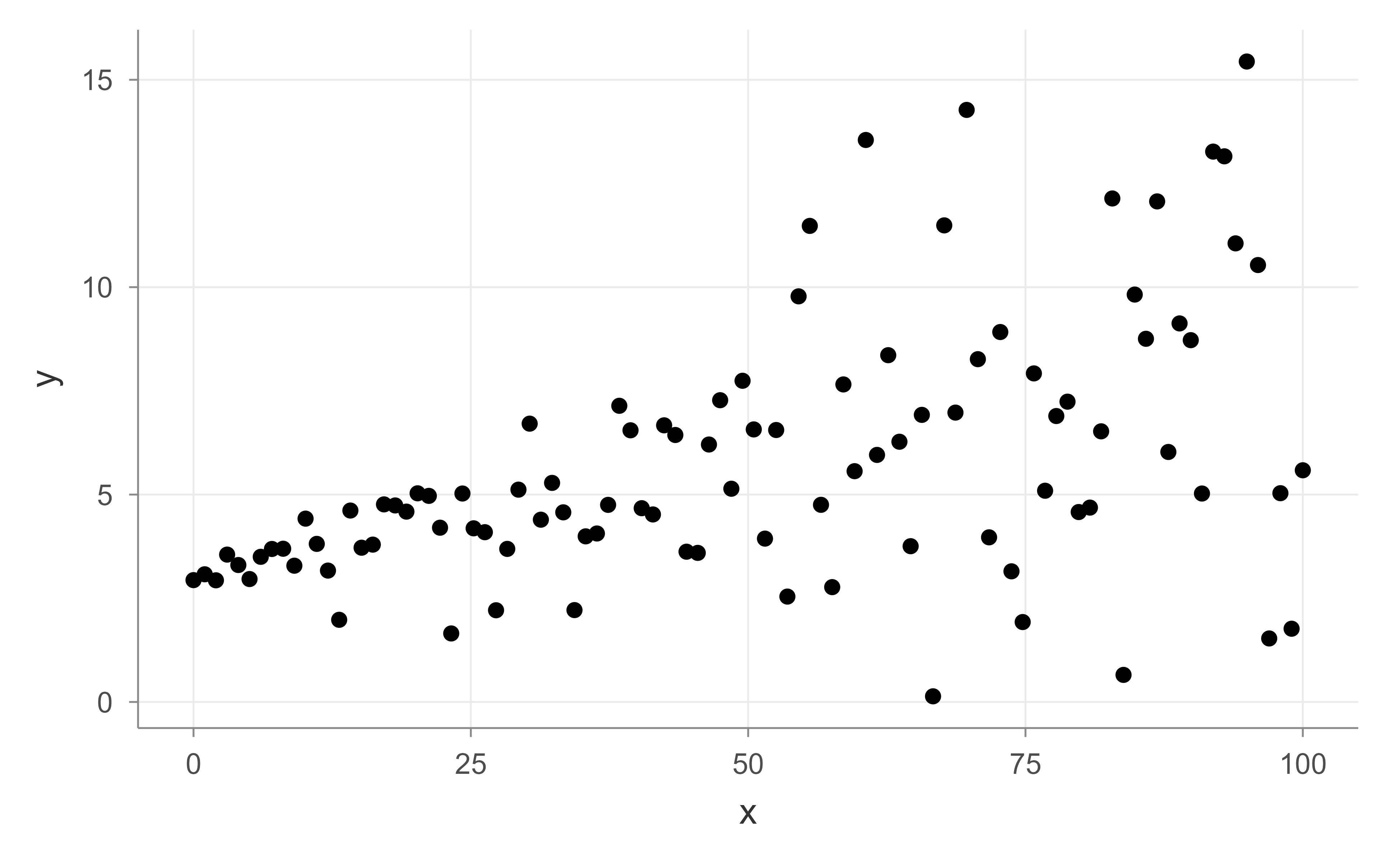
The clearest way to see what quantile regression adds is to build data where the mean line is uninformative on its own. We simulate a relationship in which the spread of $y$ grows with $x$ (heteroskedasticity, that is, non-constant variance), so the high and low quantiles fan out even though the mean trend is a simple straight line.

Show code

# generate data with non-constant variance

x <- seq(0,100,length.out = 100)        # independent variable
sig <- 0.1 + 0.05*x                     # non-constant standard deviation (sd grows with x)
b_0 <- 3                                # true intercept
b_1 <- 0.05                             # true slope
set.seed(1)                             # reproducibility
e <- rnorm(100,mean = 0, sd = sig)      # normal random error with non-constant standard deviation
y <- b_0 + b_1*x + e                    # dependent variable
dat <- data.frame(x,y)
library(ggplot2)

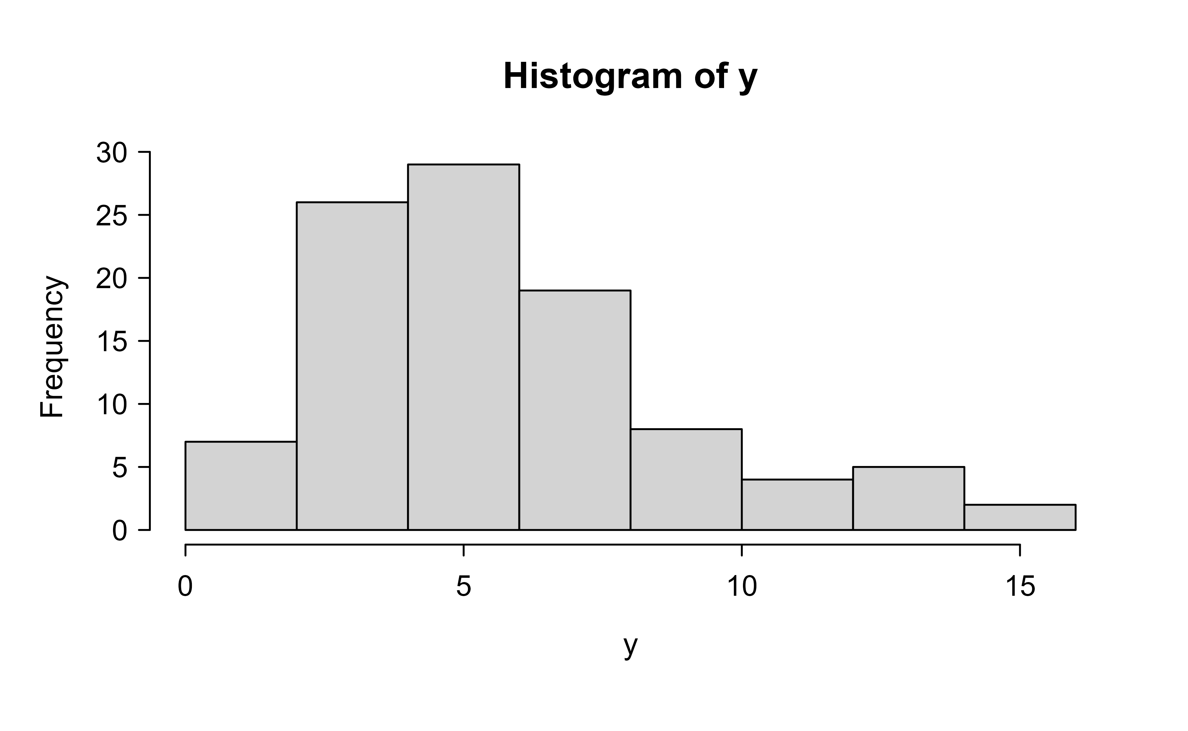
The histogram in Figure 21.1 shows the marginal distribution of the simulated outcome.

Show code

hist(y)

Figure 21.1: Histogram of the simulated outcome variable, whose spread grows with the predictor.

The scatterplot in Figure 21.2 shows the tell-tale funnel shape: points hug the line at small $x$ and spread widely at large $x$.

Show code

ggplot(dat, aes(x,y)) + geom_point()

Figure 21.2: Scatterplot of the simulated data, showing the funnel shape produced by non-constant variance.

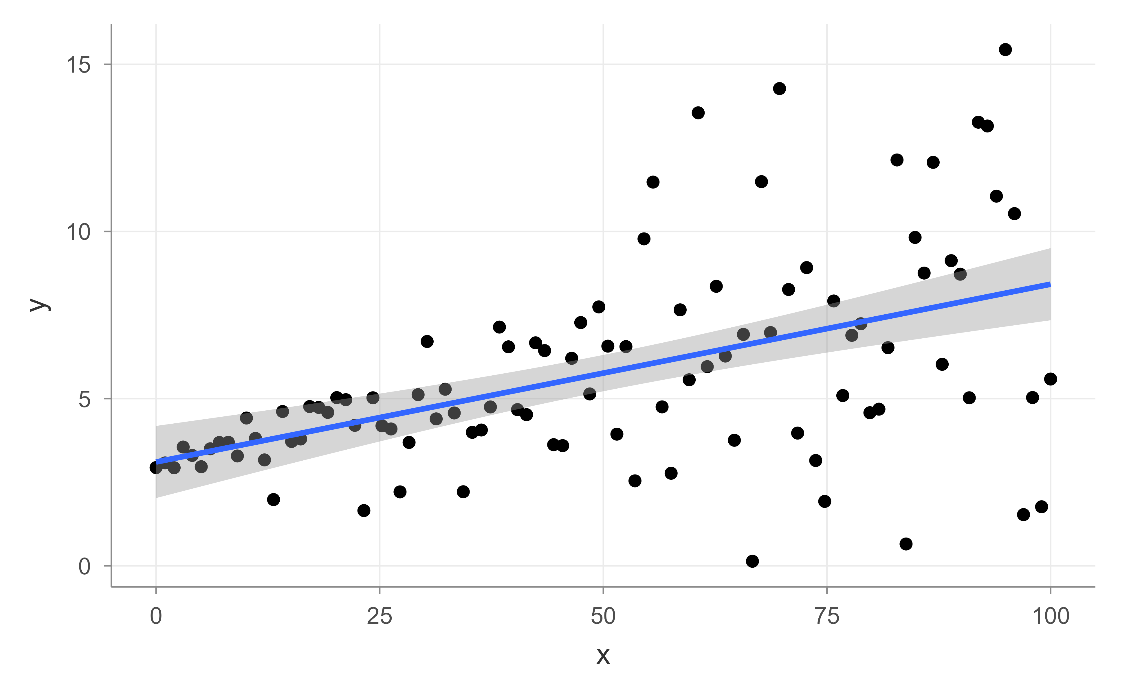
Adding the ordinary least squares line, as in Figure 21.3, captures the average trend correctly, but it says nothing about that widening spread, which is exactly the feature quantile regression is built to describe.

Show code

ggplot(dat, aes(x,y)) + geom_point() + geom_smooth(method="lm")

Figure 21.3: Simulated data with the ordinary least squares fit, which tracks the mean but ignores the changing spread.

We follow Koenker (2005) and fit a quantile regression with the quantreg package. The argument tau selects the quantile of interest; here we set it to the median.

Show code

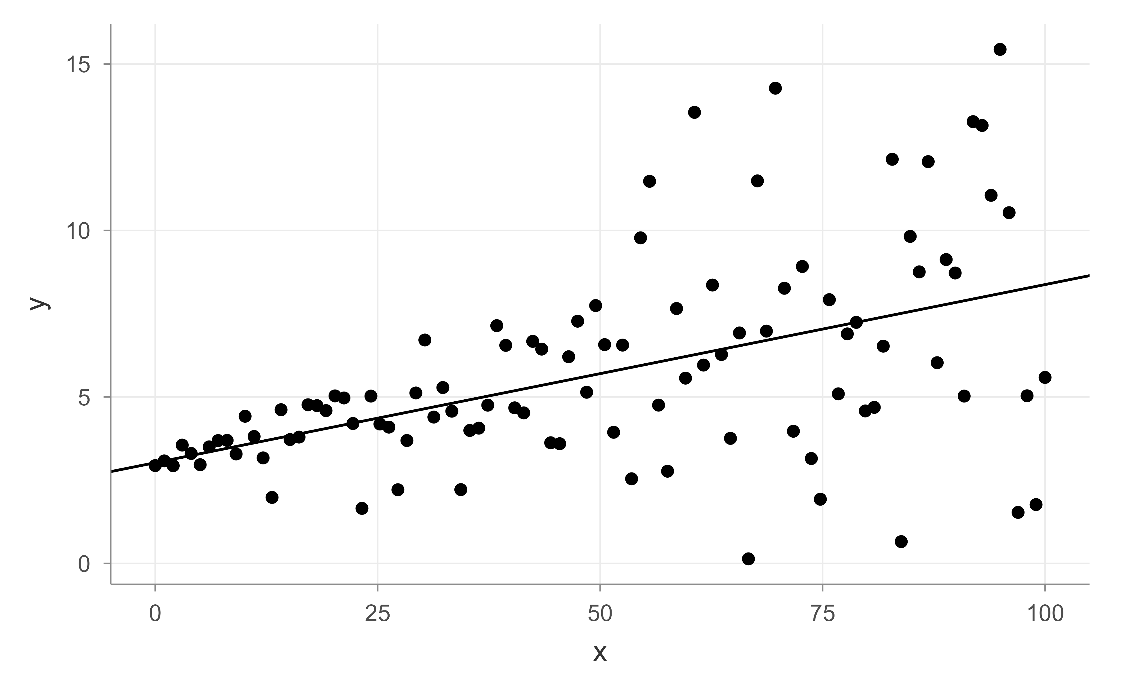
library(quantreg)
qr <- rq(y ~ x, data=dat, tau = 0.5) # tau: quantile of interest. Here we have it at 50th percentile.
summary(qr)
#> 
#> Call: rq(formula = y ~ x, tau = 0.5, data = dat)
#> 
#> tau: [1] 0.5
#> 
#> Coefficients:
#>             coefficients lower bd upper bd
#> (Intercept) 3.02410      2.80975  3.29408 
#> x           0.05351      0.03838  0.06690

The summary output reports the intercept and slope for the median fit, along with a confidence interval for each. We can draw the fitted median line on top of the data using its coefficients, as shown in Figure 21.4.

Show code

ggplot(dat, aes(x,y)) + geom_point() +
  geom_abline(intercept=coef(qr)[1], slope=coef(qr)[2])

Figure 21.4: Simulated data with the fitted median (50th percentile) quantile regression line.

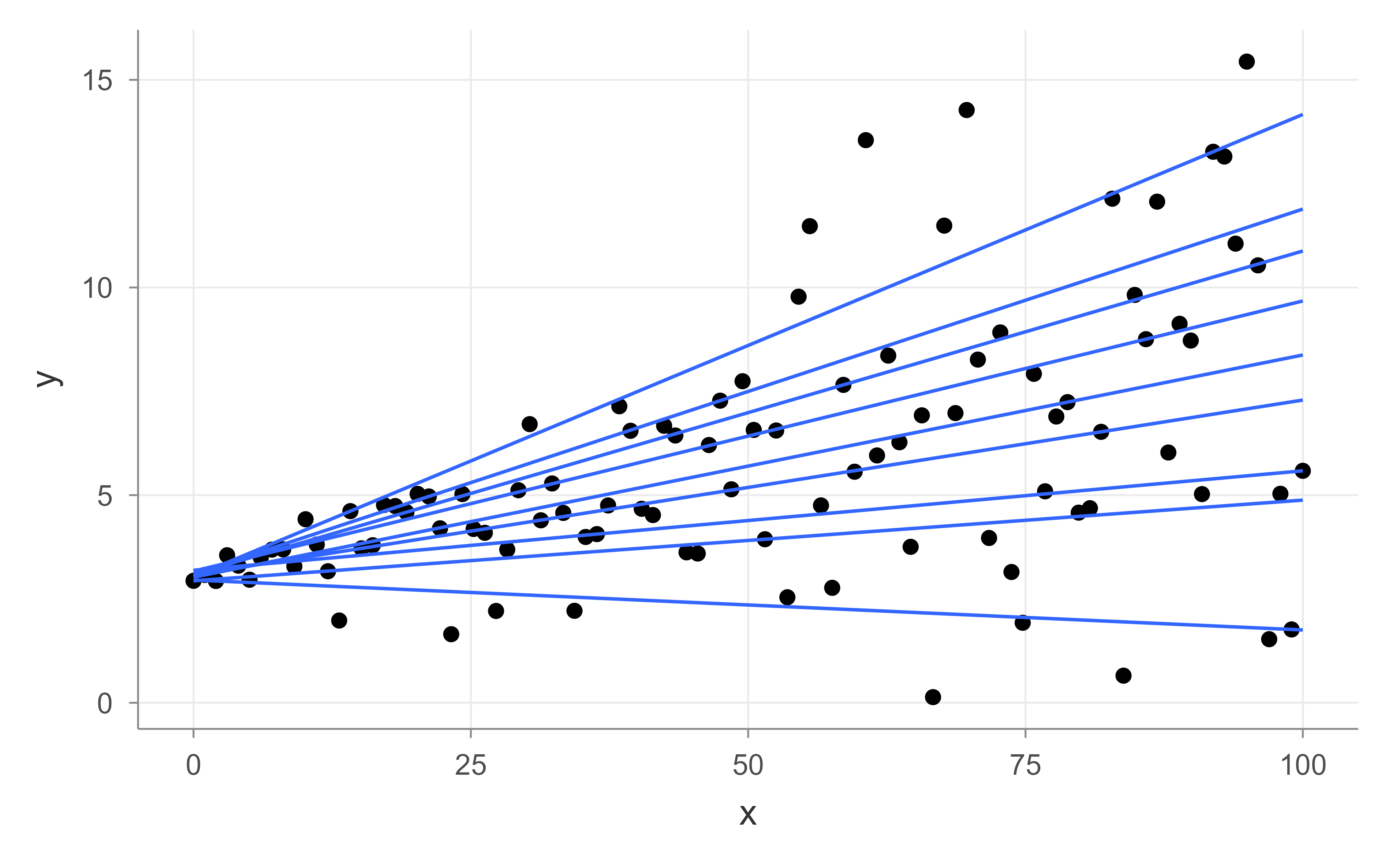
A single quantile tells only part of the story. The real value comes from fitting several quantiles at once and comparing them. We pass a vector of quantiles to tau, asking for the 10th through 90th percentiles in steps of ten.

Show code

qs <- 1:9/10
qr1 <- rq(y ~ x, data=dat, tau = qs)
#check for its coefficients
coef(qr1)
#>                tau= 0.1   tau= 0.2   tau= 0.3   tau= 0.4   tau= 0.5   tau= 0.6
#> (Intercept)  2.95735740 2.93735462 3.19112214 3.08146314 3.02409828 3.16840820
#> x           -0.01203696 0.01942669 0.02394535 0.04208019 0.05350556 0.06507385
#>               tau= 0.7   tau= 0.8 tau= 0.9
#> (Intercept) 3.09507770 3.10539343 3.041681
#> x           0.07783556 0.08782548 0.111254

# plot
ggplot(dat, aes(x,y)) + geom_point() + geom_quantile(quantiles = qs)

Figure 21.5: Simulated data with fitted quantile regression lines for the 10th through 90th percentiles, fanning out as the predictor grows.

Each line in Figure 21.5 is the fit for one quantile. Notice how they fan out as $x$ grows: the upper-quantile lines slope up more steeply and the lower-quantile lines less so, because the conditional spread of $y$ increases with $x$. That fanning is the signature of heteroskedasticity, and it is invisible in the single OLS line above.

Tip

When the quantile lines are roughly parallel, the predictor shifts the whole distribution by a constant amount and OLS already tells the full story. When they fan out or cross, the effect of $x$ depends on where in the distribution you look, and the per-quantile slopes carry information the mean cannot.

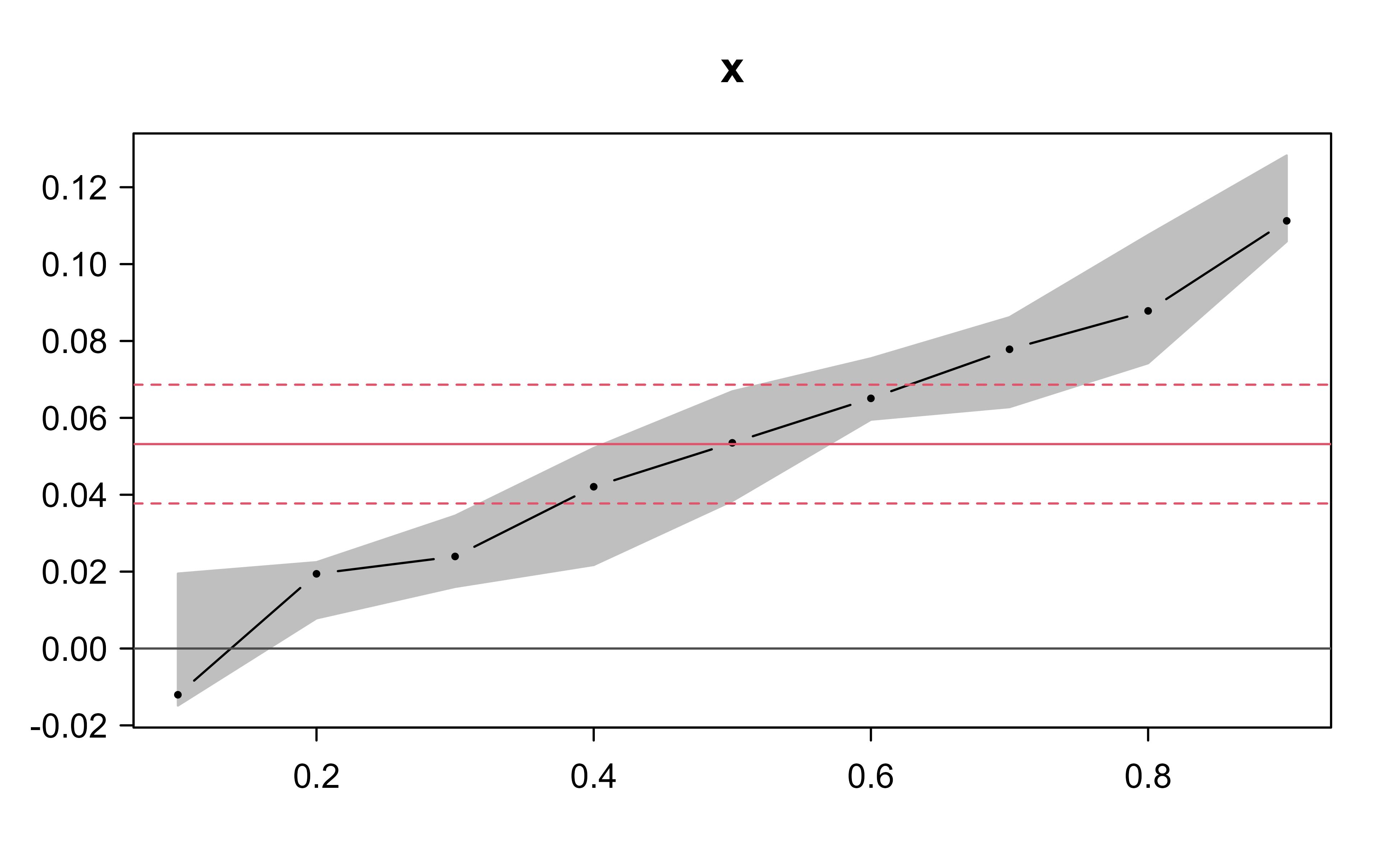
To judge whether quantile regression is telling us something beyond OLS, we can plot how each quantile coefficient varies across $q$ and overlay the OLS estimate with its confidence band, as in Figure 21.6.

Show code

plot(summary(qr1), parm="x")

Figure 21.6: Slope coefficient on the predictor across quantiles for the heteroskedastic data, with the least-squares estimate and its confidence band overlaid.

In Figure 21.6 the horizontal axis is the quantile $q$ and the vertical axis is the value of the slope coefficient on x at that quantile. The shaded region traces the quantile-regression coefficients and their confidence interval across quantiles, while the red line (with its own interval) marks the constant least-squares estimate. Here the slope clearly rises with $q$: $x$ has a larger effect on the upper quantiles than on the lower ones, consistent with the spread we built into the data.

Note

If the errors were homoskedastic and normal, the quantile slope would be (up to sampling noise) the same at every $q$, and the quantile curve would sit inside the least-squares confidence band. Departures from that flat band are the signal that the distribution’s shape, not just its level, depends on $x$.

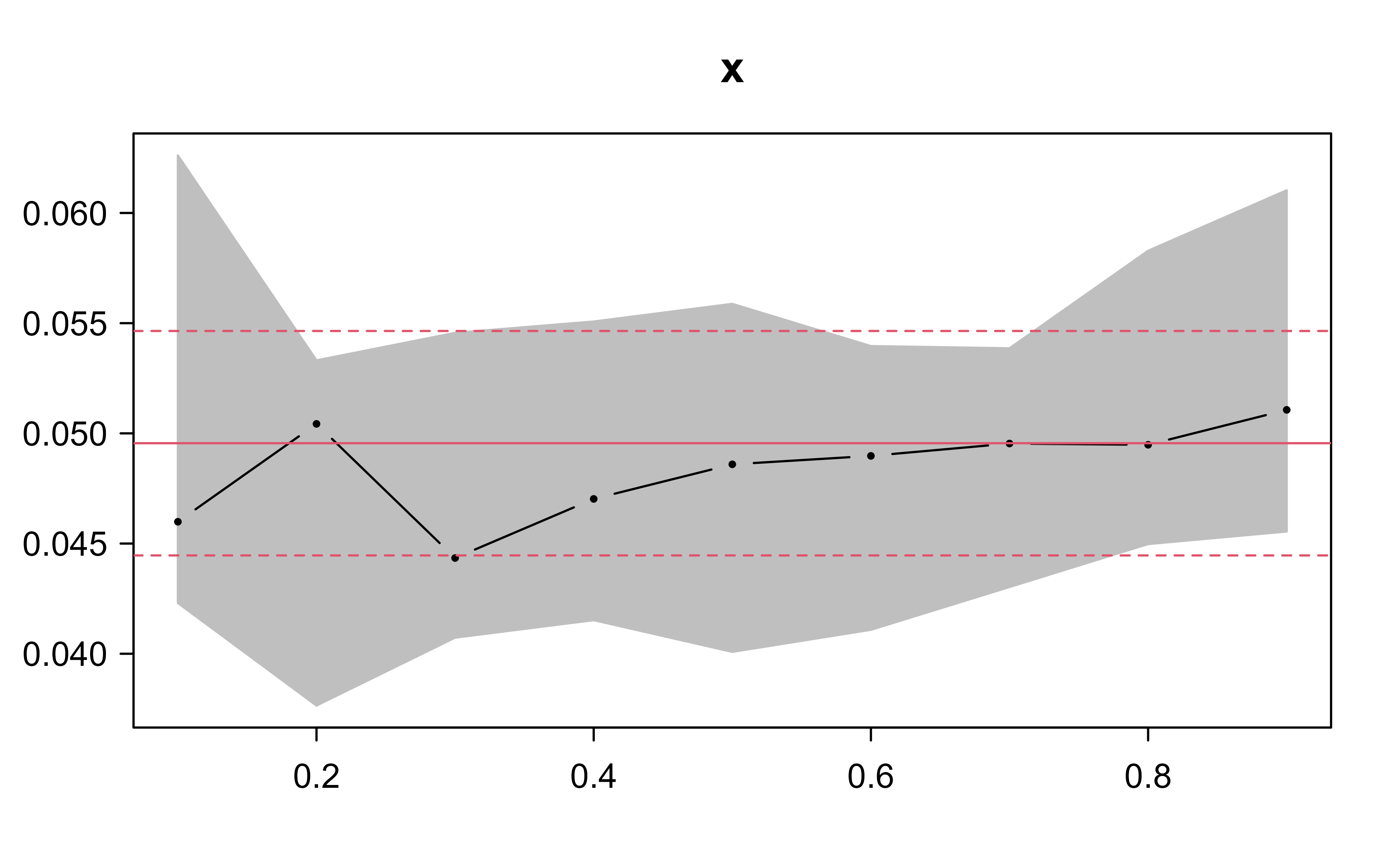
To see the contrast, we regenerate the data with constant variance and repeat the coefficient plot in Figure 21.7. Now there is no funnel: the spread of $y$ is the same for every $x$.

Show code

# generate data with constant variance

x <- seq(0, 100, length.out = 100)    # independent variable
b_0 <- 3                              # true intercept
b_1 <- 0.05                           # true slope
set.seed(1)                           # reproducibility
e <- rnorm(100, mean = 0, sd = 1)     # normal random error with constant variance
y <- b_0 + b_1 * x + e                # dependent variable
dat2 <- data.frame(x, y)
qr2 = rq(y ~ x, data = dat2, tau = qs)
plot(summary(qr2), parm = "x")

Figure 21.7: Slope coefficient on the predictor across quantiles for the homoskedastic data, lying flat within the least-squares confidence band.

This time, as Figure 21.7 shows, the quantile coefficients stay essentially flat across $q$ and lie within the least-squares band: every quantile responds to $x$ in the same way, so the mean already summarizes the relationship and quantile regression adds little. Comparing the two coefficient plots is the practical heart of the method: the first dataset shows quantile regression earning its keep, while the second shows the case where OLS suffices.

21.4 Theory, variants, and failure modes

21.4.1 Quantile crossing

Each quantile is fit by a separate optimization in Equation 21.2, with no constraint tying the fits together. Monotonicity of the true conditional quantiles ($Q_{q_1}(y\mid x) \le Q_{q_2}(y\mid x)$ for $q_1 < q_2$) is therefore not guaranteed in the estimated fits: two fitted lines for different $q$ can cross, implying the absurd conclusion that a lower quantile exceeds a higher one for some $x$. This is most common at extreme $q$, in sparse regions of the design, or far from the data centroid where the linear extrapolation is least trustworthy. Two standard remedies exist. The first is rearrangement (Chernozhukov, Fernandez-Val, and Galichon, 2010): at any fixed $x$, sort the estimated $\{\hat Q_q(y\mid x)\}_q$ into increasing order; the sorted curve is a valid, monotone quantile function and is provably at least as accurate (in $L_p$) as the unsorted one. The second is to fit all quantiles jointly under non-crossing constraints. Crossing is a diagnostic as much as a nuisance: heavy crossing inside the data range signals that the linear-in-$x$ specification is inadequate.

21.4.2 Connections to other methods

Quantile regression sits inside several larger families. It is an M-estimator with the non-smooth, asymmetric score $\psi_q$ of Equation 21.4, which is why the asymptotics in Equation 21.6 take the standard sandwich form. It has an exact Bayesian reading through the asymmetric Laplace distribution (ALD): the negative log-likelihood of an ALD with location $x'\beta$ and asymmetry $q$ is, up to constants, proportional to the check loss, so maximizing that likelihood reproduces Equation 21.2 and a prior on $\beta$ yields a posterior whose mode is the penalized quantile estimate. This connects to the regularized variants: adding an $\ell_1$ penalty gives the LASSO quantile regression (rq with method="lasso" or the rqPen package),

\[ \hat\beta_q^{\text{lasso}} = \arg\min_\beta \sum_{i=1}^N \rho_q\!\left(y_i - x_i'\beta\right) + \lambda \sum_{j=2}^p |\beta_j|, \]

which remains a linear program (both pieces are piecewise linear) and performs simultaneous quantile estimation and variable selection. Beyond linearity, the check loss can be paired with splines (additive quantile models), with kernels and gradient boosting (quantile loss is the objective behind prediction-interval forests and gradient-boosted quantile estimators), and with the pinball loss used to train neural networks that output predictive quantiles. Finally, the estimated quantiles are natural ingredients for distribution-free prediction intervals, the link to conformal methods drawn in Chapter 85.

21.4.3 Failure modes

Beyond the ties-and-zeros caveat already raised, three failure modes deserve emphasis. First, tail estimation is intrinsically hard: by Equation 21.7 the variance scales like $1/f(F^{-1}(q))^2$, which blows up as $q \to 0$ or $q \to 1$ because the density thins, so a “90th-percentile slope” from a few hundred observations can be very imprecise even when the median slope is sharp. Second, the linear specification can be locally wrong even when it is right on average; because each quantile is fit independently, a misspecified mean shape shows up as systematic crossing or as quantile curves that are individually implausible. Third, inference is delicate: the asymptotic variance depends on the unknown sparsity $1/f$, and naive plug-in density estimates can be unstable, which is why the rank-score or bootstrap standard errors are usually preferred to the i.i.d. formula in finite samples.

21.4.4 Verifying the population result

The derivation in Section 21.2.2 predicts that the minimizer of the average check loss over a sample is the corresponding empirical quantile. We can confirm this directly with base R, with no model matrix at all.

Show code

set.seed(1)
z  <- rnorm(2000)
qq <- 0.8
check <- function(t) mean(ifelse(z >= t, qq*(z - t), (qq - 1)*(z - t)))
t_hat <- optimize(check, interval = range(z))$minimum
c(check_loss_minimizer = t_hat, empirical_quantile = unname(quantile(z, qq)))
#> check_loss_minimizer   empirical_quantile 
#>            0.8695729            0.8680546

The check-loss minimizer matches the empirical 0.8 quantile (and both track the theoretical value qnorm(0.8) $\approx 0.842$), exactly as Equation 21.3 and the first-order condition require.

To sum up, quantile regression generalizes the familiar mean model by targeting any quantile of the outcome through an asymmetric absolute-error loss. It is robust to outliers, makes no distributional assumption on the errors, and is invariant to monotone transformations. Its real strength shows up when the effect of a predictor varies across the distribution: by fitting and comparing many quantiles, we recover the changing spread and shape that a single mean line conceals. Estimated quantiles also serve as building blocks for distribution-free prediction intervals, a connection developed further in the conformal prediction chapter (Chapter 85).

A mean sits between the modes of a bimodal distribution, in a region where few observations actually live, so it describes no typical case well. Separate quantile fits can track each part of the distribution.↩︎
This is why, for example, you can model $\log y$ and then exponentiate the fitted quantiles to recover quantiles of $y$ directly, with no smearing correction of the kind OLS requires.↩︎
The piecewise-linear, convex objective makes this a well-behaved optimization: a global optimum always exists, and efficient specialized algorithms handle even large problems.↩︎

# Quantile Regression {#sec-quantile-reg} ```{r} #| include: false source("_common.R") ``` Ordinary least squares answers one question very well: given the predictors, what is the *average* value of the outcome? The fitted line traces the conditional mean, $E(y|x)$, and a single slope summarizes how that average moves as $x$ moves. That is often exactly what we want. But the average can hide a great deal. Two groups of patients might have the same mean recovery time while one group has a long, heavy upper tail of slow recoverers that a clinic cares about most. A pay-equity study might find no difference in mean salary across groups while the gap is large at the top of the pay scale and absent at the bottom. In both cases the interesting action is in the *shape* of the distribution, not its center, and the mean alone cannot see it. Quantile regression widens the lens. Instead of modeling only the mean, it models any quantile (any percentile) of the outcome distribution as a function of the predictors. We can ask how the 10th percentile of $y$ responds to $x$, how the median responds, how the 90th percentile responds, and compare those answers. When the relationship is the same at every quantile, quantile regression simply reproduces the OLS story. When it differs, quantile regression reveals structure (changing spread, skewness, effects that grow in the tails) that a mean model averages away. ::: {.callout-important title="Key idea"} OLS estimates the conditional mean $E(y|x)$. Quantile regression estimates a conditional quantile $Q_q(y|x)$, the value below which a fraction $q$ of the outcome falls at each setting of $x$. Sweeping $q$ from near 0 to near 1 gives a family of fits that describes the whole conditional distribution, not just its center. ::: In this chapter you will learn what a conditional quantile is and why we might prefer it to the mean, how the model is fit by minimizing an asymmetric absolute-error loss (the "tilted" or "check" loss), how to read the resulting coefficients, and how to estimate and visualize quantile fits in R with the `quantreg` package. The classic reference for the method is @Roger_1996; for an accessible academic review see @Yu_2003. The most familiar special case is the median. When $q = 0.5$, quantile regression becomes median regression, also called least-absolute-deviations (LAD) regression, which chooses the line minimizing the sum of absolute residuals $\sum_{i}|e_i|$ rather than the sum of squared residuals. Because absolute errors do not square large deviations, the median fit is far less sensitive to a few extreme points than the mean fit is. ::: {.callout-tip title="Intuition"} OLS minimizes *squared* errors, so a single far-away point can drag the whole line toward it. LAD (median) regression minimizes *absolute* errors, so an outlier counts in proportion to its distance rather than its distance squared. That is the same reason the median of a list of numbers barely moves when you replace its largest value with something ten times larger, while the mean lurches. ::: ## Why and when to use it It helps to be explicit about what quantile regression buys you and what it costs, before getting into the mechanics. The main attractions are these. Quantile regression is more robust to outliers than OLS, because it rests on absolute rather than squared loss. It gives a fuller picture of the data, describing how the entire conditional distribution shifts with the predictors rather than reporting a single average effect, which is especially valuable when the outcome is skewed or has a bimodal or multimodal distribution (several humps with several modes) that a mean would misrepresent.^[A mean sits between the modes of a bimodal distribution, in a region where few observations actually live, so it describes no typical case well. Separate quantile fits can track each part of the distribution.] It makes no parametric assumption about the error distribution: we do not have to claim the errors are normal or anything else, which connects it to the nonparametric view of the outcome's full distribution taken up in the density estimation chapter (@sec-density-estimation). And it has a clean equivariance property that OLS lacks: quantiles are preserved under monotone transformations, so the $q$th quantile of $g(y)$ is $g$ applied to the $q$th quantile of $y$ for any increasing $g$. OLS does not share this, since in general $E(g(y)) \neq g(E(y))$.^[This is why, for example, you can model $\log y$ and then exponentiate the fitted quantiles to recover quantiles of $y$ directly, with no smearing correction of the kind OLS requires.] The estimated coefficients also behave well for inference: under standard conditions the quantile-regression estimator $\hat\beta$ is asymptotically normally distributed, which lets us attach standard errors and confidence intervals. ::: {.callout-tip title="When to use this"} Reach for quantile regression when you care about more than the average, when the outcome is skewed or heavy-tailed, when effects plausibly differ across the distribution (small at the median, large in the tail), or when outliers make an OLS mean untrustworthy. (When the outliers themselves are the object of interest rather than a nuisance, see the anomaly and outlier detection chapter, @sec-anomaly-detection.) ::: There is one practical limitation worth flagging. Quantile regression works best when the outcome is continuous. If the dependent variable has many tied values or piles of zeros (so that whole ranges of the distribution sit at a single number), individual quantiles become poorly identified and the method is less informative. ::: {.callout-warning} Avoid quantile regression when the outcome is discrete with heavy ties or has a large mass of zeros (for example, count or censored data with many zeros). The quantiles you are trying to estimate may not be uniquely defined there. ::: ## The model and its loss function The model looks like a linear regression, but the coefficient vector now depends on the quantile $q$ we have chosen to target: $$ y_i = x_i'\beta_q + e_i $$ Everything hinges on how we measure the error. Write the residual as $e(x) = y - \hat{y}(x)$, and let $L(e(x)) = L(y - \hat{y}(x))$ be the loss we pay for that error. OLS uses squared loss; here we start from absolute loss. If $L(e) = |e|$, the absolute-error loss function, then $\hat\beta$ is found by minimizing $\sum_i |y_i - x_i'\beta|$, which is exactly median (LAD) regression. To target a quantile other than the median, we tilt this absolute loss so that under-prediction and over-prediction are penalized differently. The objective function for quantile $q$ is $$ Q(\beta_q)=\sum_{i:y_i \ge x_i'\beta}^{N} q|y_i - x_i'\beta_q| + \sum_{i:y_i < x_i'\beta}^{N} (1-q)|y_i-x_i'\beta_q| $$ where $0 < q < 1$. The first sum collects the points lying *above* the fitted line (where we under-predicted) and weights their absolute errors by $q$; the second sum collects the points *below* the line (where we over-predicted) and weights theirs by $1 - q$. ::: {.callout-tip title="Intuition"} This asymmetric weighting is what pins the fit to a particular quantile. Suppose $q = 0.9$. Then under-prediction costs $0.9$ per unit of error while over-prediction costs only $0.1$. To keep the total small, the line is pushed up until about 90% of the points sit below it, which is precisely the definition of the 90th percentile. Set $q = 0.5$ and the two weights are equal, the loss is symmetric, and we recover median regression. ::: Because $|e|$ has a kink at zero, the objective is not differentiable, so there is no closed-form normal-equation solution as in OLS. Instead the problem is solved as a linear program, classically with the simplex method, and standard errors are commonly obtained by the bootstrap rather than from a formula.^[The piecewise-linear, convex objective makes this a well-behaved optimization: a global optimum always exists, and efficient specialized algorithms handle even large problems.] ### Precise formulation: the check loss {#sec-quantile-reg-formulation} To reason about the estimator we need notation that is both compact and exact. Define the *check function* (also called the pinball or tilted absolute loss) at level $q \in (0,1)$, $$ \rho_q(u) = u\bigl(q - \mathbb{1}\{u < 0\}\bigr) = \begin{cases} q\,u, & u \ge 0,\\[2pt] (q-1)\,u, & u < 0, \end{cases} $$ {#eq-quantile-reg-check} where $\mathbb{1}\{\cdot\}$ is the indicator. Both branches are nonnegative: for $u \ge 0$ the loss is $qu \ge 0$, and for $u < 0$ the loss is $(q-1)u = (1-q)|u| \ge 0$. The objective $Q(\beta_q)$ written out term by term above is exactly $\sum_{i=1}^N \rho_q\!\left(y_i - x_i'\beta_q\right)$, with the two summation ranges corresponding to the two branches of @eq-quantile-reg-check. The quantile-regression estimator is $$ \hat\beta_q = \arg\min_{\beta \in \mathbb{R}^p} \sum_{i=1}^N \rho_q\!\left(y_i - x_i'\beta\right). $$ {#eq-quantile-reg-estimator} The *conditional quantile* being estimated is defined through the conditional distribution function $F_{y|x}$: the $q$th conditional quantile is $$ Q_q(y \mid x) = \inf\{\, t : F_{y\mid x}(t) \ge q \,\} = F_{y\mid x}^{-1}(q), $$ {#eq-quantile-reg-cqf} and the linear model asserts $Q_q(y\mid x) = x'\beta_q$. Crucially this is a *model of the quantile*, not of the mean plus an additive error of fixed shape: nothing requires the errors $e_i = y_i - x_i'\beta_q$ to be identically distributed or symmetric, only that the $q$th conditional quantile of $e_i$ given $x_i$ be zero, that is $\Pr(e_i \le 0 \mid x_i) = q$. This single restriction is the entire stochastic assumption. ### Why minimizing the check loss returns a quantile {#sec-quantile-reg-derivation} The asymmetric weighting story is correct but informal. Here is the derivation that makes it exact, first for the unconditional case (an intercept-only model), which already contains the whole idea. Let $Y$ be a random variable with distribution function $F$ and consider choosing a single number $t$ to minimize the expected check loss, $$ R(t) = \mathbb{E}\,\rho_q(Y - t) = q\!\int_{t}^{\infty}\!(y-t)\,dF(y) \;+\; (1-q)\!\int_{-\infty}^{t}\!(t-y)\,dF(y). $$ Differentiate with respect to $t$. Using Leibniz's rule (the integrand vanishes at the moving endpoint $y=t$, so only the explicit $t$ inside the integrands contributes), $$ R'(t) = -q\!\int_{t}^{\infty}\! dF(y) + (1-q)\!\int_{-\infty}^{t}\! dF(y) = -q\bigl(1 - F(t)\bigr) + (1-q)F(t). $$ Setting $R'(t)=0$ and solving, $$ -q + qF(t) + F(t) - qF(t) = 0 \;\Longrightarrow\; F(t) = q, $$ so the minimizer satisfies $F(t) = q$, that is $t = F^{-1}(q)$, the $q$th quantile. The second derivative is $R''(t) = f(t) \ge 0$ wherever the density exists, confirming a minimum, and convexity of $\rho_q$ guarantees it is the global one. Setting $q = \tfrac12$ recovers $F(t) = \tfrac12$, the median, and the symmetric absolute loss. This is the population analogue of the fact that the sample check-loss minimizer puts a fraction $q$ of points below the fit. For the regression case the same calculation runs on the subgradient. Because $\rho_q$ is convex but kinked at $0$, $\hat\beta_q$ is characterized by the condition that the zero vector lies in the subdifferential of @eq-quantile-reg-estimator. Away from the kink, $\rho_q'(u) = q - \mathbb{1}\{u<0\} = \psi_q(u)$, and the optimality (normal-equation analogue) condition is $$ \sum_{i=1}^N x_i\,\psi_q\!\left(y_i - x_i'\hat\beta_q\right) = 0, \qquad \psi_q(u) = q - \mathbb{1}\{u < 0\}, $$ {#eq-quantile-reg-foc} with the residuals that are exactly zero contributing subgradient values in $[\,q-1,\,q\,]$ chosen to balance the sum. Compare this to the OLS normal equation $\sum_i x_i(y_i - x_i'\hat\beta) = 0$: quantile regression replaces the raw residual by the *bounded, sign-and-tilt* score $\psi_q$, which is why a far-away point exerts influence only through its sign, not its magnitude. That bounded score is the precise source of the robustness claimed earlier. A useful corollary of @eq-quantile-reg-foc: take the row corresponding to the intercept, where $x_{i1}=1$. Then $\sum_i \psi_q(\hat e_i) = 0$, i.e. $q N$ equals the number of strictly negative residuals plus a fractional contribution from the exact zeros. In general position a fitted quantile plane interpolates exactly $p$ observations (the residuals at those points are zero), and a fraction approximately $q$ of the remaining residuals are negative. This is the regression generalization of "the median has half the data on each side." ::: {.callout-note} "Not differentiable" sounds like trouble but is not. The loss is still convex, so the optimization is reliable; we just use linear-programming machinery instead of calculus. The `quantreg` package handles all of this for you. ::: ### Interpreting the coefficients The payoff of all this is an interpretation that parallels OLS but applies at a chosen point of the distribution. For the $j$th predictor $x_j$, the coefficient is the marginal effect on the $q$th conditional quantile: $$ \frac{\partial Q_q(y|x)}{\partial x_j} = \beta_{qj} $$ In words: at the $q$th quantile of $y$, a one-unit increase in $x_j$ is associated with a $\beta_{qj}$-unit change in $y$, holding the other predictors fixed. The reading is the same sentence you would write for an OLS slope, with one addition: it applies *at that quantile* rather than to the average. ::: {.callout-important title="Key idea"} A single OLS regression gives you one slope per predictor. Quantile regression run across many values of $q$ gives you a *curve* of slopes, one per quantile, showing whether a predictor matters more at the bottom, the middle, or the top of the outcome distribution. ::: ### The linear-programming representation {#sec-quantile-reg-lp} The claim that @eq-quantile-reg-estimator "is a linear program" can be made literal, which both explains how `rq` computes the fit and exposes the dual that drives inference. Split each residual into its positive and negative parts, $u_i = (y_i - x_i'\beta)^+ \ge 0$ and $v_i = (y_i - x_i'\beta)^- \ge 0$, so that $y_i - x_i'\beta = u_i - v_i$ and $\rho_q(y_i - x_i'\beta) = q\,u_i + (1-q)\,v_i$. The estimation problem becomes the linear program $$ \min_{\beta,\,u,\,v}\; q\,\mathbf{1}'u + (1-q)\,\mathbf{1}'v \quad\text{s.t.}\quad X\beta + u - v = y,\;\; u \ge 0,\;\; v \ge 0, $$ {#eq-quantile-reg-lp} with $\beta$ free. This has $N$ equality constraints and $2N + p$ variables; its solution is a basic feasible point at which $p$ residuals are zero, recovering the interpolation property noted above. The classical solver is a simplex method specialized to this structure (Barrodale to Roberts, used by `rq(method="br")`, exact and excellent for small to moderate $N$); for large $N$ an interior-point method with preprocessing (`method="pfn"` or the Frisch to Newton variant) scales much better. The dual variables $a_i$ of @eq-quantile-reg-lp lie in $[q-1,\,q]$ and are the "regression rank scores" used by one family of inference procedures. ::: {.callout-note} The cost of a single quantile fit is comparable to that of a least-squares fit for moderate sizes: $O(N p^2)$-ish for the linear algebra, with the simplex overhead. Fitting a whole grid of quantiles is cheap because `rq` can warm-start each fit from the neighboring one (the entire solution path in $q$ is itself piecewise constant in $\beta$, and `rq(tau=-1)` returns it exactly via parametric programming). ::: ### Asymptotic distribution and inference {#sec-quantile-reg-asymptotics} The estimator is consistent and asymptotically normal under mild conditions (continuous conditional density positive at the quantile, finite design moments). Writing $\beta_q$ for the truth and $f_{y\mid x}$ for the conditional density of $y$, the standard result (@Roger_1996) is $$ \sqrt{N}\,\bigl(\hat\beta_q - \beta_q\bigr) \;\xrightarrow{d}\; \mathcal{N}\!\left(0,\; \tau\,(1-\tau)\,D_1^{-1} D_0\, D_1^{-1}\right), $$ {#eq-quantile-reg-asymp} with $\tau = q$, $D_0 = \mathbb{E}\!\left[x x'\right]$ and the *sparsity-weighted* matrix $$ D_1 = \mathbb{E}\!\left[\,f_{y\mid x}\!\bigl(x'\beta_q \mid x\bigr)\, x x'\,\right]. $$ The sandwich has the same algebraic shape as in M-estimation: the meat $\tau(1-\tau)D_0$ is the variance of the score $\psi_q$ (note $\operatorname{Var}\psi_q = q(1-q)$), and the bread $D_1^{-1}$ is the inverse expected Jacobian. The density factor $f_{y\mid x}$ inside $D_1$ is the catch: precision degrades where the conditional density is low, so estimates in the far tails (small or large $q$) are noisier, and the reciprocal density $1/f$ is called the *sparsity function*. In the special case of i.i.d. errors with density $f$, $D_1 = f(F^{-1}(q))\,D_0$ and the covariance collapses to the textbook form $$ \operatorname{Avar}(\hat\beta_q) = \frac{q(1-q)}{N\,f\!\left(F^{-1}(q)\right)^2}\,D_0^{-1}, $$ {#eq-quantile-reg-iid-avar} which is exactly the LAD/median result with the familiar $1/(2f(\text{median}))$ scale at $q=\tfrac12$. The practical difficulty is estimating $f(F^{-1}(q))$; `summary.rq` offers several routes: a difference-quotient (Siddiqui to Hall to Sheather) estimate of the sparsity (`se="nid"` for the non-i.i.d. sandwich, `se="iid"` for @eq-quantile-reg-iid-avar), the rank-score inversion (`se="rank"`, which avoids density estimation entirely and gives the confidence intervals shown by default), and the bootstrap (`se="boot"`), which is the most robust default when in doubt. ## Application The clearest way to see what quantile regression adds is to build data where the mean line is uninformative on its own. We simulate a relationship in which the *spread* of $y$ grows with $x$ (heteroskedasticity, that is, non-constant variance), so the high and low quantiles fan out even though the mean trend is a simple straight line. ```{r} # generate data with non-constant variance x <- seq(0,100,length.out = 100) # independent variable sig <- 0.1 + 0.05*x # non-constant standard deviation (sd grows with x) b_0 <- 3 # true intercept b_1 <- 0.05 # true slope set.seed(1) # reproducibility e <- rnorm(100,mean = 0, sd = sig) # normal random error with non-constant standard deviation y <- b_0 + b_1*x + e # dependent variable dat <- data.frame(x,y) library(ggplot2) ``` The histogram in @fig-quantile-reg-hist shows the marginal distribution of the simulated outcome. ```{r fig-quantile-reg-hist, fig.cap="Histogram of the simulated outcome variable, whose spread grows with the predictor."} hist(y) ``` The scatterplot in @fig-quantile-reg-scatter shows the tell-tale funnel shape: points hug the line at small $x$ and spread widely at large $x$. ```{r fig-quantile-reg-scatter, fig.cap="Scatterplot of the simulated data, showing the funnel shape produced by non-constant variance."} ggplot(dat, aes(x,y)) + geom_point() ``` Adding the ordinary least squares line, as in @fig-quantile-reg-ols, captures the average trend correctly, but it says nothing about that widening spread, which is exactly the feature quantile regression is built to describe. ```{r fig-quantile-reg-ols, fig.cap="Simulated data with the ordinary least squares fit, which tracks the mean but ignores the changing spread."} ggplot(dat, aes(x,y)) + geom_point() + geom_smooth(method="lm") ``` We follow @Roger_1996 and fit a quantile regression with the `quantreg` package. The argument `tau` selects the quantile of interest; here we set it to the median. ```{r} library(quantreg) qr <- rq(y ~ x, data=dat, tau = 0.5) # tau: quantile of interest. Here we have it at 50th percentile. summary(qr) ``` The `summary` output reports the intercept and slope for the median fit, along with a confidence interval for each. We can draw the fitted median line on top of the data using its coefficients, as shown in @fig-quantile-reg-median. ```{r fig-quantile-reg-median, fig.cap="Simulated data with the fitted median (50th percentile) quantile regression line."} ggplot(dat, aes(x,y)) + geom_point() + geom_abline(intercept=coef(qr)[1], slope=coef(qr)[2]) ``` A single quantile tells only part of the story. The real value comes from fitting several quantiles at once and comparing them. We pass a vector of quantiles to `tau`, asking for the 10th through 90th percentiles in steps of ten. ```{r fig-quantile-reg-fan, fig.cap="Simulated data with fitted quantile regression lines for the 10th through 90th percentiles, fanning out as the predictor grows."} qs <- 1:9/10 qr1 <- rq(y ~ x, data=dat, tau = qs) #check for its coefficients coef(qr1) # plot ggplot(dat, aes(x,y)) + geom_point() + geom_quantile(quantiles = qs) ``` Each line in @fig-quantile-reg-fan is the fit for one quantile. Notice how they fan out as $x$ grows: the upper-quantile lines slope up more steeply and the lower-quantile lines less so, because the conditional spread of $y$ increases with $x$. That fanning is the signature of heteroskedasticity, and it is invisible in the single OLS line above. ::: {.callout-tip} When the quantile lines are roughly parallel, the predictor shifts the whole distribution by a constant amount and OLS already tells the full story. When they fan out or cross, the effect of $x$ depends on where in the distribution you look, and the per-quantile slopes carry information the mean cannot. ::: To judge whether quantile regression is telling us something beyond OLS, we can plot how each quantile coefficient varies across $q$ and overlay the OLS estimate with its confidence band, as in @fig-quantile-reg-coef-hetero. ```{r fig-quantile-reg-coef-hetero, fig.cap="Slope coefficient on the predictor across quantiles for the heteroskedastic data, with the least-squares estimate and its confidence band overlaid."} plot(summary(qr1), parm="x") ``` In @fig-quantile-reg-coef-hetero the horizontal axis is the quantile $q$ and the vertical axis is the value of the slope coefficient on `x` at that quantile. The shaded region traces the quantile-regression coefficients and their confidence interval across quantiles, while the red line (with its own interval) marks the constant least-squares estimate. Here the slope clearly rises with $q$: $x$ has a larger effect on the upper quantiles than on the lower ones, consistent with the spread we built into the data. ::: {.callout-note} If the errors were homoskedastic and normal, the quantile slope would be (up to sampling noise) the same at every $q$, and the quantile curve would sit inside the least-squares confidence band. Departures from that flat band are the signal that the distribution's shape, not just its level, depends on $x$. ::: To see the contrast, we regenerate the data with *constant* variance and repeat the coefficient plot in @fig-quantile-reg-coef-homo. Now there is no funnel: the spread of $y$ is the same for every $x$. ```{r fig-quantile-reg-coef-homo, fig.cap="Slope coefficient on the predictor across quantiles for the homoskedastic data, lying flat within the least-squares confidence band."} # generate data with constant variance x <- seq(0, 100, length.out = 100) # independent variable b_0 <- 3 # true intercept b_1 <- 0.05 # true slope set.seed(1) # reproducibility e <- rnorm(100, mean = 0, sd = 1) # normal random error with constant variance y <- b_0 + b_1 * x + e # dependent variable dat2 <- data.frame(x, y) qr2 = rq(y ~ x, data = dat2, tau = qs) plot(summary(qr2), parm = "x") ``` This time, as @fig-quantile-reg-coef-homo shows, the quantile coefficients stay essentially flat across $q$ and lie within the least-squares band: every quantile responds to $x$ in the same way, so the mean already summarizes the relationship and quantile regression adds little. Comparing the two coefficient plots is the practical heart of the method: the first dataset shows quantile regression earning its keep, while the second shows the case where OLS suffices. ## Theory, variants, and failure modes {#sec-quantile-reg-advanced} ### Quantile crossing {#sec-quantile-reg-crossing} Each quantile is fit by a separate optimization in @eq-quantile-reg-estimator, with no constraint tying the fits together. Monotonicity of the true conditional quantiles ($Q_{q_1}(y\mid x) \le Q_{q_2}(y\mid x)$ for $q_1 < q_2$) is therefore not guaranteed in the *estimated* fits: two fitted lines for different $q$ can cross, implying the absurd conclusion that a lower quantile exceeds a higher one for some $x$. This is most common at extreme $q$, in sparse regions of the design, or far from the data centroid where the linear extrapolation is least trustworthy. Two standard remedies exist. The first is *rearrangement* (Chernozhukov, Fernandez-Val, and Galichon, 2010): at any fixed $x$, sort the estimated $\{\hat Q_q(y\mid x)\}_q$ into increasing order; the sorted curve is a valid, monotone quantile function and is provably at least as accurate (in $L_p$) as the unsorted one. The second is to fit all quantiles jointly under non-crossing constraints. Crossing is a diagnostic as much as a nuisance: heavy crossing inside the data range signals that the linear-in-$x$ specification is inadequate. ### Connections to other methods {#sec-quantile-reg-connections} Quantile regression sits inside several larger families. It is an *M-estimator* with the non-smooth, asymmetric score $\psi_q$ of @eq-quantile-reg-foc, which is why the asymptotics in @eq-quantile-reg-asymp take the standard sandwich form. It has an exact *Bayesian* reading through the asymmetric Laplace distribution (ALD): the negative log-likelihood of an ALD with location $x'\beta$ and asymmetry $q$ is, up to constants, proportional to the check loss, so maximizing that likelihood reproduces @eq-quantile-reg-estimator and a prior on $\beta$ yields a posterior whose mode is the penalized quantile estimate. This connects to the regularized variants: adding an $\ell_1$ penalty gives the *LASSO quantile regression* (`rq` with `method="lasso"` or the `rqPen` package), $$ \hat\beta_q^{\text{lasso}} = \arg\min_\beta \sum_{i=1}^N \rho_q\!\left(y_i - x_i'\beta\right) + \lambda \sum_{j=2}^p |\beta_j|, $$ which remains a linear program (both pieces are piecewise linear) and performs simultaneous quantile estimation and variable selection. Beyond linearity, the check loss can be paired with splines (additive quantile models), with kernels and gradient boosting (quantile loss is the objective behind prediction-interval forests and gradient-boosted quantile estimators), and with the pinball loss used to train neural networks that output predictive quantiles. Finally, the estimated quantiles are natural ingredients for distribution-free prediction intervals, the link to conformal methods drawn in @sec-conformal-prediction. ### Failure modes {#sec-quantile-reg-failure} Beyond the ties-and-zeros caveat already raised, three failure modes deserve emphasis. First, *tail estimation is intrinsically hard*: by @eq-quantile-reg-iid-avar the variance scales like $1/f(F^{-1}(q))^2$, which blows up as $q \to 0$ or $q \to 1$ because the density thins, so a "90th-percentile slope" from a few hundred observations can be very imprecise even when the median slope is sharp. Second, *the linear specification can be locally wrong even when it is right on average*; because each quantile is fit independently, a misspecified mean shape shows up as systematic crossing or as quantile curves that are individually implausible. Third, *inference is delicate*: the asymptotic variance depends on the unknown sparsity $1/f$, and naive plug-in density estimates can be unstable, which is why the rank-score or bootstrap standard errors are usually preferred to the i.i.d. formula in finite samples. ### Verifying the population result {#sec-quantile-reg-verify} The derivation in @sec-quantile-reg-derivation predicts that the minimizer of the average check loss over a sample is the corresponding empirical quantile. We can confirm this directly with base R, with no model matrix at all. ```{r} set.seed(1) z <- rnorm(2000) qq <- 0.8 check <- function(t) mean(ifelse(z >= t, qq*(z - t), (qq - 1)*(z - t))) t_hat <- optimize(check, interval = range(z))$minimum c(check_loss_minimizer = t_hat, empirical_quantile = unname(quantile(z, qq))) ``` The check-loss minimizer matches the empirical 0.8 quantile (and both track the theoretical value `qnorm(0.8)` $\approx 0.842$), exactly as @eq-quantile-reg-cqf and the first-order condition require. To sum up, quantile regression generalizes the familiar mean model by targeting any quantile of the outcome through an asymmetric absolute-error loss. It is robust to outliers, makes no distributional assumption on the errors, and is invariant to monotone transformations. Its real strength shows up when the effect of a predictor varies across the distribution: by fitting and comparing many quantiles, we recover the changing spread and shape that a single mean line conceals. Estimated quantiles also serve as building blocks for distribution-free prediction intervals, a connection developed further in the conformal prediction chapter (@sec-conformal-prediction).