| Property | Batch | Online |
|---|---|---|
| When prediction runs | Scheduled job, ahead of need | Per request, on demand |
| Latency seen by caller | None (precomputed lookup) | Milliseconds in request path |
| Input freshness | As stale as last run | Always current input |
| Compute cost shape | Large, predictable, parallel | Small per call, must hold capacity |
| Failure blast radius | Whole run, but offline | Live traffic, immediate |
| Scaling concern | Throughput of the job | Tail latency and concurrency |
| Typical use | Churn scores, nightly risk, recommendations cache | Fraud check at checkout, dynamic pricing, search ranking |
116 Model Deployment and Serving
A fitted model that lives only in an R session has no users. You can call predict() on it at your desk, but nobody else can, and the moment you close the session it is gone. Deployment is the work of turning that trained object into a service: something other systems can call repeatedly, safely, and in a way you can update without breaking the callers who depend on it. Think of the difference between cooking a meal for yourself and running a kitchen that serves the same dish to hundreds of strangers, on demand, every day, without you in the room. The recipe is the same; almost everything else changes.
This chapter is about that handoff. We will look at the two basic serving patterns (batch versus online), the layered tooling in the R ecosystem (vetiver, plumber, Docker, Posit Connect), the contract a serving endpoint exposes to its callers, and the rollout strategies (versioned endpoints, A/B testing, canary releases) that let you change a model in production without taking down the system or silently degrading predictions. By the end you should be able to reason about when to serve a model in real time versus precompute it, what an endpoint must promise its callers, and how to ship a new version without betting the whole system on it.
The mechanics of wrapping a function as an HTTP endpoint were introduced in the API chapter (Chapter 107), and packaging that endpoint into a portable image was covered in the containerizing chapter (Chapter 106). This chapter assumes both and focuses on the decisions around them: when to serve in real time versus in batch, how to keep the request and response format stable, and how to ship a new version with controlled risk.
Note
This chapter is about serving a frozen model, not about training it. Choosing and fitting the model happened in earlier chapters. Here the model is a given, and the questions are all operational: where it runs, who calls it, and how you change it safely.
116.1 Where Deployment Fits in the Workflow
A predictive system has a lifecycle: explore, train, evaluate, package, deploy, monitor (Chapter 117), retrain. Everything before “deploy” happens in an interactive session and is reversible at no cost. If you make a mistake while exploring, you fix a line and rerun. Everything from “deploy” onward touches infrastructure that other teams and end users depend on, and mistakes there are visible and expensive: a bad deploy can degrade a live product before anyone notices. Deployment is the boundary between a model as an analysis artifact and a model as a production dependency, and crossing it changes the cost of being wrong.
Two properties make this boundary worth treating carefully. The first is that the training environment and the serving environment are different processes, often on different machines, running at different times. A prediction made at serving time must reproduce exactly what the model would have produced at training time on the same input. Any drift in package versions, factor levels, column order, or preprocessing breaks this silently: the endpoint still returns a number, it is just the wrong number. This kind of mismatch is known as training/serving skew, and it is the most common source of bugs that pass every unit test and still ruin predictions.
The second property is that callers form a contract with the endpoint. Once a dashboard or a downstream service sends requests in a particular shape and parses responses in a particular shape, you cannot change that shape without coordinating with every caller. A model you can edit freely; a public interface you cannot. Much of what follows is really about contract discipline rather than statistics.
Key idea
Training produces three things you must ship together: the fitted parameters, the preprocessing that maps raw inputs to model inputs, and the metadata that pins the environment (R version, package versions, input schema). The serving process loads all three and does nothing else heavy. If any one of the three is missing or stale, the served model quietly stops matching the trained model.
This is the same separation-of-concerns argument from the API chapter, made stricter: at serving time the goal is to do as little as possible beyond loading a self-contained artifact and calling predict() on validated input.
116.2 Batch Versus Online Serving
The first deployment decision is when predictions are produced relative to when they are consumed. There are two regimes, and most systems use one or sometimes both. The intuition is simple: either you compute predictions ahead of time and look them up, or you compute them on the spot when someone asks.
In batch serving, you score a large set of rows on a schedule (nightly, hourly) and write the predictions to a table or file. Consumers read the precomputed predictions; the model is never in the request path. Picture a bakery that bakes everything overnight and stocks the shelves: customers grab what is already there, instantly, but only from what was baked. This is cheap per prediction, trivially parallel, and easy to reason about, but predictions are as stale as the last run, and you cannot score an input that did not exist when the batch ran.
In online (real-time) serving, the model sits behind an endpoint and scores one request at a time as it arrives. This is the made-to-order kitchen: the dish is fresh and tailored to the request, but someone has to be standing at the stove, fast, whenever an order comes in. Online serving gives fresh predictions on inputs you have never seen, at the cost of latency budgets, capacity planning, and the operational burden of keeping a service healthy.
Warning
“Online serving” here means real-time request scoring with a fixed model. It is distinct from online learning (the online and streaming learning chapter, Chapter 55), where the model parameters themselves update as data arrive. A real-time endpoint usually serves a frozen model and is retrained out of band. Confusing the two leads people to expect an endpoint to “learn” from traffic when it is doing nothing of the kind.
Table 116.1 lays out the two regimes side by side along the properties that usually drive the choice between them.
A frequent and sensible hybrid combines the two: precompute predictions in batch for the common, slow-moving cases (and cache them), then stand up an online endpoint only for the long tail of fresh inputs the cache misses. This keeps the expensive online path small while still covering inputs the batch never saw.
Tip
When you are unsure which regime you need, start by asking whether the inputs exist before the prediction is needed. If every input you will ever score is already known (an existing customer list, a fixed product catalog), batch is almost always simpler and cheaper. Only reach for online serving when inputs are genuinely created at request time.
116.2.1 A Cost Model for Choosing
The choice is not only about freshness; it is also about cost, and the cost comparison can be made precise. Suppose you must serve predictions for a population, and at any moment a fraction \(r\) of that population is actually queried before the next batch refresh. Let \(N\) be the population size, \(c_b\) the cost to score one row in batch, and \(c_o\) the cost to score one row online (typically \(c_o > c_b\) because online carries per-request overhead). Batch scores everyone every cycle; online scores only what is asked.
\[ C_{\text{batch}} = N \, c_b, \qquad C_{\text{online}} = r \, N \, c_o . \]
Online is cheaper when \(r \, N \, c_o < N \, c_b\), that is when
\[ r < \frac{c_b}{c_o}. \]
So when the queried fraction \(r\) is small relative to the per-unit cost ratio, pay only for what you use and serve online; when nearly everyone is queried (\(r \to 1\)), batch wins because it avoids the per-request overhead and amortizes setup.1 The freshness requirement can override this arithmetic, but the arithmetic is the right starting point. Figure 116.1 visualizes this break-even: the online cost rises with the queried fraction while the batch cost is flat, and the two cross at \(r = c_b/c_o\).
Show code
N  <- 1e6      # population size
cb <- 1        # cost units to score one row in batch
co <- 4        # cost units to score one row online (higher per-call overhead)

r <- seq(0, 1, length.out = 201)
cost_batch  <- rep(N * cb, length(r))
cost_online <- r * N * co

breakeven <- cb / co  # r at which the two are equal

plot(r, cost_online, type = "l", lwd = 2,
     xlab = "Queried fraction r",
     ylab = "Total cost (arbitrary units)",
     main = "Batch vs online serving cost")
lines(r, cost_batch, lwd = 2, lty = 2)
abline(v = breakeven, col = "grey50", lty = 3)
legend("topleft",
       legend = c("Online (r * N * co)", "Batch (N * cb)",
                  sprintf("break-even r = %.2f", breakeven)),
       lwd = c(2, 2, 1), lty = c(1, 2, 3),
       col = c("black", "black", "grey50"), bty = "n")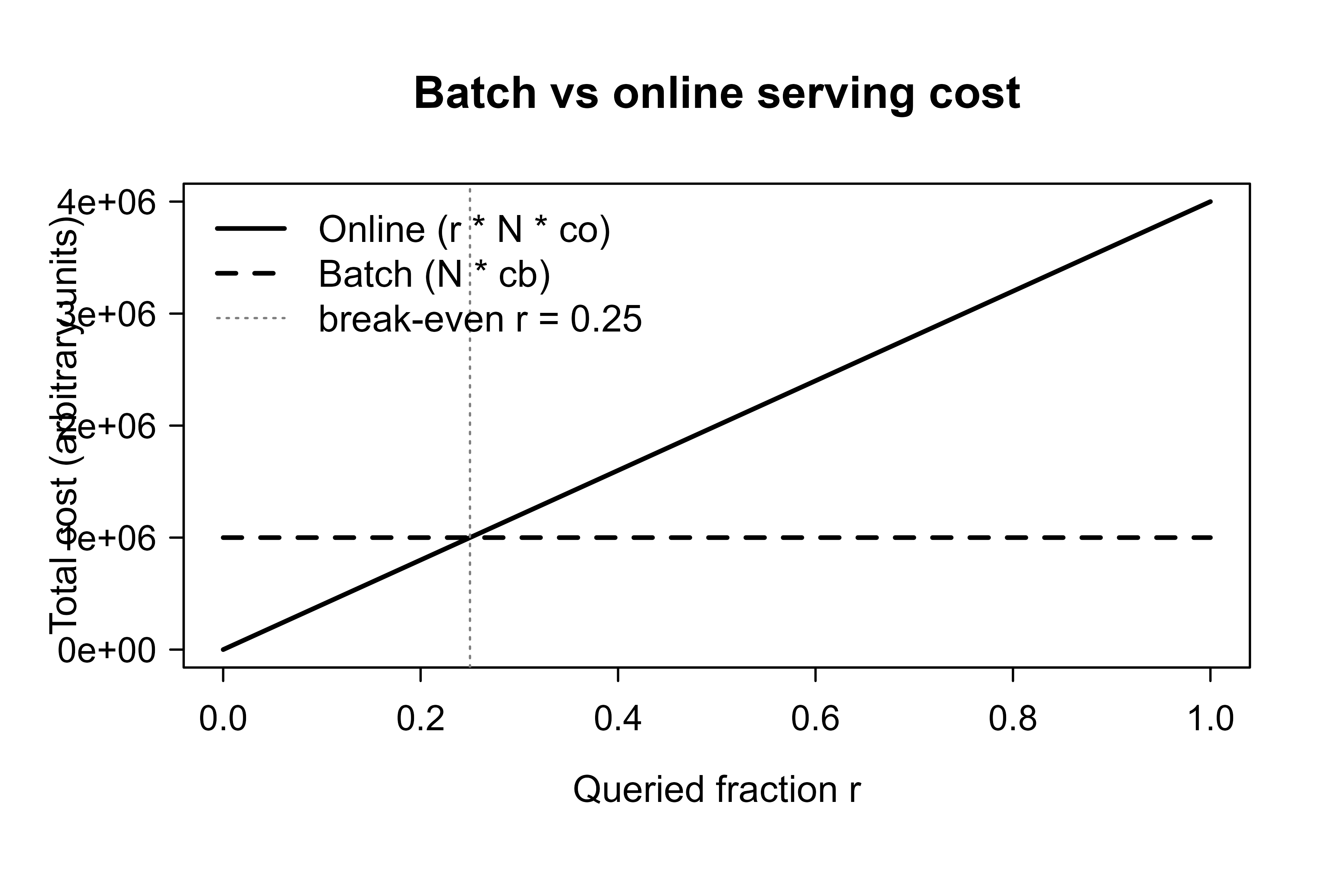
116.3 The REST Contract
Having decided to serve a model online, the next question is what, exactly, the endpoint promises to the world. That promise is the contract: the agreement between server and callers about the request format, the response format, and the error behavior. The contract, not the model, is what callers depend on. You can swap a random forest for a gradient boosting model freely as long as the contract holds, and conversely, a tiny change to the response shape can break a dashboard even though the model is untouched.
Intuition
A serving endpoint is like a power socket. Appliances do not care how the electricity is generated, only that the voltage and the plug shape stay fixed. Callers do not care which algorithm you use, only that the request and response keep their agreed shape.
A minimal prediction contract has these parts, each of which a caller will eventually depend on:
- Method and path. Conventionally
POST /predict, plus aGET /health(or/ping) for liveness checks that a load balancer can poll. - Request schema. The set of input fields, their types, whether each is required, and accepted ranges or factor levels. JSON is the usual encoding.
- Response schema. A predictable structure, for example
{"prediction": [...], "model_version": "..."}. Returning the model version inside the response is valuable: a caller (or a log) can later tell which model produced a given prediction. - Error semantics. What status code and body you return when the input is malformed (a
400with a message naming the bad field), versus when the server itself fails (a500). Callers write retry and alerting logic against these codes, so they must be stable. - Versioning. A way to address a specific version of the model, usually in the path (
/v2/predict) or a header.
Of all these parts, the single most important property is input validation at the boundary. A model will happily extrapolate on garbage: feed a logistic regression an age of \(-5\) or a category it never saw, and it will still return a confident-looking probability. The endpoint must therefore reject inputs that violate the schema before they reach the model. This is the same idea as the data validation chapter (Chapter 104), applied at the request boundary.
Warning
An endpoint that does not validate its input does not fail loudly; it fails quietly, returning plausible numbers for nonsense inputs. Silent wrong answers are far more dangerous than visible errors, because nobody knows to investigate them.
The runnable demo at the end of this chapter implements exactly this validation step in base R, so the logic is visible without any framework.
116.4 Tooling: vetiver, plumber, Docker, Posit Connect
You do not have to build all of this by hand. The R ecosystem has a layered set of tools for serving, each handling one part of the problem, and they compose like a stack: a higher layer hands its output to the layer below it. Table 116.2 summarizes the stack from the fitted object at the top to a hosted endpoint at the bottom.
| Layer | Tool | Responsibility |
|---|---|---|
| Model packaging + metadata | vetiver (+ pins) | Bundle fitted model, preprocessing, input schema, version; store and retrieve |
| HTTP endpoint | plumber | Turn predict functions into a REST API with an OpenAPI spec |
| Portable runtime | Docker | Pin R version, system libs, packages, and code into one image |
| Hosting + lifecycle | Posit Connect / cloud | Run the image, route traffic, manage versions, expose URLs, monitor |
116.4.1 vetiver: model to API
vetiver packages a fitted model together with the metadata needed to serve it (the prediction method, the input prototype that defines the schema, and a version string), stores it in a pins board (a local folder, a cloud bucket, or Posit Connect), and can generate the plumber API and the Dockerfile for you. In other words, it automates the “ship three things together” rule from the start of the chapter: the fitted object, the schema, and the environment metadata all travel as one versioned artifact. It removes most of the hand-written glue from the API chapter (Chapter 107) and the containerizing chapter (Chapter 106).
When to use this
Reach for vetiver when you want the standard, opinionated path (model plus schema plus version plus API plus Dockerfile) generated for you. Drop to hand-written plumber and Docker only when you need control the generator does not give.
The flow below shows the path end to end. It requires vetiver and pins, which are not in the runnable set here, so the chunk is eval=FALSE, but it is current, idiomatic code.
Show code
library(vetiver)
library(pins)

# A fitted model from anywhere (base R, tidymodels, etc.).
fit <- lm(mpg ~ wt + hp, data = mtcars)

# Wrap it: vetiver captures the predict method, an input prototype
# (the schema, inferred from the training data), and a version.
v <- vetiver_model(fit, model_name = "mtcars_mpg")

# Store it in a versioned board. Each pin_write creates a new version.
board <- board_folder(path = "vetiver_board", versioned = TRUE)
vetiver_pin_write(board, v)

# Build a plumber router with /predict, /ping, and an OpenAPI page.
library(plumber)
pr() |>
  vetiver_api(v) |>
  pr_run(port = 8080)
To serve a specific version (the heart of versioned endpoints), read that version back from the board rather than the latest:
Show code
# List versions and pin one explicitly.
versions <- pin_versions(board, "mtcars_mpg")
v_old <- vetiver_pin_read(board, "mtcars_mpg",
                          version = versions$version[1])

# vetiver can also write the Dockerfile and the plumber.R for you,
# so the image build is reproducible.
vetiver_prepare_docker(board, name = "mtcars_mpg",
                       docker_args = list(port = 8080))
116.4.2 plumber, Docker, Posit Connect
When you need control beyond what vetiver generates, write the plumber.R by hand as in the API chapter, build the Docker image as in the Containerizing chapter, and deploy the image. Posit Connect is the managed host in the Posit stack: it accepts a plumber API (or a vetiver model pinned to it), gives it a URL, holds multiple versions, and provides access control and basic usage telemetry. vetiver_deploy_rsconnect() pushes a pinned model to Connect directly. The same image can equally run on any container platform (Kubernetes, a cloud run service); Connect is a convenience, not a requirement.
116.5 Versioned Endpoints and Rollout Strategies
Getting a model live is the easy part; the hard part comes later, when you need to change it. The naive approach, overwriting the running model with a new one, is a blind, all-at-once switch: if the new model is worse, every caller feels it immediately, and you have no comparison to tell you it got worse. Mature deployment avoids this by combining versioned endpoints with a controlled rollout.
Versioned endpoints keep more than one model addressable at once. The new model is deployed alongside the old one (for example at /v2/predict while /v1/predict keeps serving), and traffic is moved deliberately rather than flipped. The payoff is that rollback becomes a routing change instead of a redeploy: if /v2 misbehaves, you point traffic back at /v1 in seconds.
Key idea
You cannot roll back safely to a version you did not keep. Versioned endpoints exist so that the previous, known-good model is always one routing change away.
With more than one version live, two rollout strategies sit on top of versioning. They look similar (both split traffic) but answer different questions:
- Canary. Send a small fraction of live traffic (say 5 percent) to the new version, watch its error rate and prediction quality, and increase the fraction only if it holds up.2 The blast radius of a bad model is bounded by the canary fraction. This is a risk-control mechanism.
- A/B test. Split traffic between two versions to measure which produces better downstream outcomes (conversion, revenue, click-through), with the split held long enough to reach statistical significance. This is a measurement mechanism, not just a safety valve.
Warning
Do not use a canary to decide which model is “better.” A canary runs briefly on little traffic, which is fine for catching crashes but far too little data to measure a small business lift. Measuring lift is the job of an A/B test, and the next section shows why it needs so much more traffic.
Table 116.3 contrasts the three rollout strategies by their goal, traffic split, decision rule, and main risk.
| Strategy | Goal | Traffic split | Decision rule | Main risk |
|---|---|---|---|---|
| Blue/green | Instant cutover with instant rollback | 100% old, then 100% new | Switch when new passes smoke tests | Cutover bug hits everyone at once |
| Canary | Limit risk of a bad release | Small % to new, ramped up | Promote if metrics stay healthy at each step | Slow to surface rare failures |
| A/B test | Decide which model is better on a business metric | Fixed split (e.g. 50/50) held for the test | Promote the arm with the better metric at significance | Needs enough traffic and time for power |
116.5.1 How Much Traffic an A/B Test Needs
An A/B test is a hypothesis test, so its required size follows from the usual power calculation. Suppose the metric is a conversion rate, with baseline rate \(p\) under the current model, and you want to detect an absolute improvement \(\delta\) to \(p + \delta\). For a two-sided test at significance level \(\alpha\) and power \(1 - \beta\), the approximate sample size per arm is
\[ n \;\approx\; \frac{\left(z_{1-\alpha/2} + z_{1-\beta}\right)^2 \, \bigl[\, p(1-p) + (p+\delta)(1-p-\delta) \,\bigr]}{\delta^2}, \]
where \(z_q\) is the \(q\) quantile of the standard normal.3 The \(\delta^2\) in the denominator is the key fact: detecting a smaller lift costs quadratically more traffic. Halving the lift you want to detect roughly quadruples the sample you need.
Intuition
Small effects hide in noise. To be confident that a 1 percent improvement is real and not luck, you need enough data that random fluctuations average out below 1 percent, and that takes a great deal more traffic than confirming a 4 percent improvement. This is why canarying (a safety decision, needing little data) and A/B testing (a measurement decision, needing a lot) are genuinely different activities even though both split traffic.
Figure 116.2 plots this relationship: the required sample size per arm climbs steeply as the lift to detect shrinks, reflecting the \(\delta^2\) in the denominator.
Show code
ab_n_per_arm <- function(p, delta, alpha = 0.05, power = 0.80) {
  z_a <- qnorm(1 - alpha / 2)
  z_b <- qnorm(power)
  num <- (z_a + z_b)^2 * (p * (1 - p) + (p + delta) * (1 - p - delta))
  num / delta^2
}

p <- 0.10
deltas <- seq(0.005, 0.05, by = 0.001)
ns <- sapply(deltas, function(d) ab_n_per_arm(p, d))

plot(deltas, ns, type = "l", lwd = 2,
     xlab = "Absolute lift to detect (delta)",
     ylab = "Required n per arm",
     main = "A/B test size vs effect size")
points(deltas[seq(1, length(deltas), by = 5)],
       ns[seq(1, length(deltas), by = 5)], pch = 19, cex = 0.6)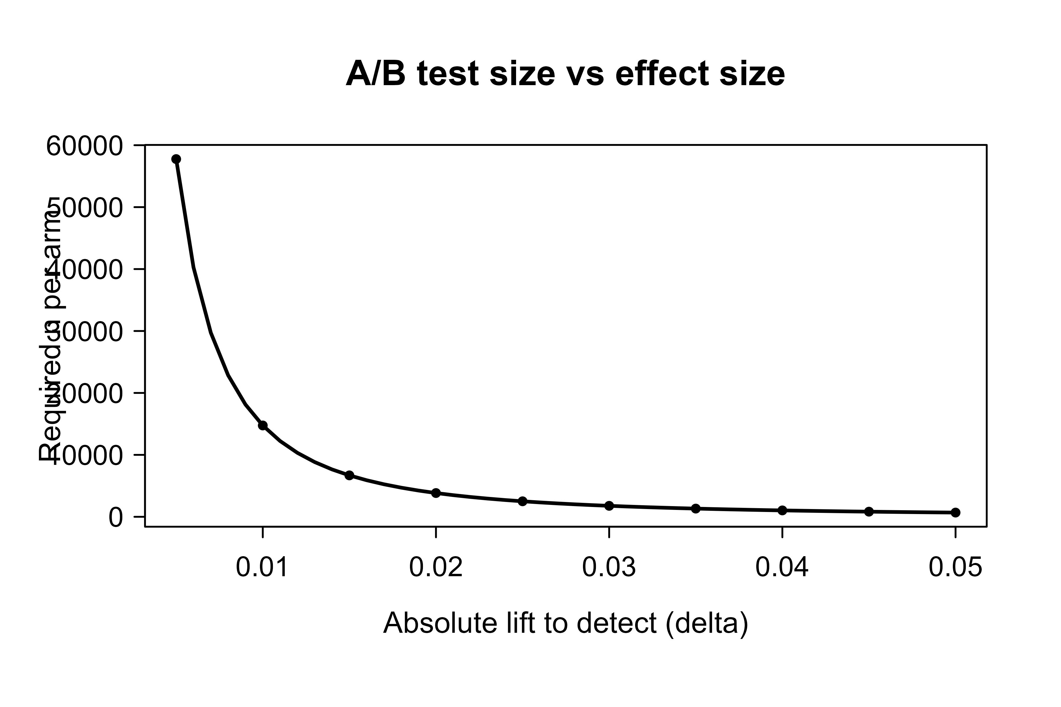
116.6 Runnable Demo: Serialize a Model and a Validating Predict Wrapper
It is easy to lose the core ideas inside the conveniences of vetiver and plumber, so this section strips them away. The core of any deployment is just two operations: persist a fitted model to disk so a separate process can load it, and wrap its predict in a function that validates inputs against a schema before scoring. Everything the frameworks do is an elaboration of these two steps. The demo below is pure base R so the mechanics are fully visible, and it runs end to end.
We train a small logistic model, serialize it with saveRDS, then build a predict wrapper that enforces an input schema: required columns present, correct types, values in range, factor levels recognized. Invalid rows are rejected with an informative error (the analogue of a 400 response); valid rows are scored.
Show code
set.seed(1)

# --- Train a simple model -------------------------------------------------
n <- 300
train <- data.frame(
  age    = round(runif(n, 18, 80)),
  income = round(rlnorm(n, log(40000), 0.5)),
  region = factor(sample(c("north", "south", "east", "west"), n, TRUE))
)
# True relationship plus noise -> binary outcome.
lp <- -3 + 0.03 * train$age + 0.00002 * train$income +
      ifelse(train$region == "south", 0.5, 0)
train$y <- rbinom(n, 1, plogis(lp))

fit <- glm(y ~ age + income + region, data = train, family = binomial())

# --- Serialize the model + its schema -------------------------------------
# A deployable artifact is the model plus the metadata needed to validate
# inputs. We capture a schema from the training data and a version string.
schema <- list(
  age    = list(type = "numeric", min = 18,  max = 120),
  income = list(type = "numeric", min = 0,   max = 1e7),
  region = list(type = "factor",  levels = levels(train$region))
)
artifact <- list(
  model   = fit,
  schema  = schema,
  version = "1.0.0"
)

path <- tempfile(fileext = ".rds")
saveRDS(artifact, path)

# --- Load in a (conceptually separate) serving process --------------------
served <- readRDS(path)

# --- Input validation against the schema ----------------------------------
validate_input <- function(newdata, schema) {
  errors <- character(0)

  # 1. Required columns present.
  missing_cols <- setdiff(names(schema), names(newdata))
  if (length(missing_cols) > 0) {
    errors <- c(errors,
                paste0("missing required field(s): ",
                       paste(missing_cols, collapse = ", ")))
  }

  # 2. Per-field type and range / level checks (only for present fields).
  for (field in intersect(names(schema), names(newdata))) {
    spec <- schema[[field]]
    val  <- newdata[[field]]

    if (spec$type == "numeric") {
      if (!is.numeric(val)) {
        errors <- c(errors, paste0("field '", field, "' must be numeric"))
        next
      }
      if (any(val < spec$min | val > spec$max, na.rm = TRUE)) {
        errors <- c(errors,
                    paste0("field '", field, "' out of range [",
                           spec$min, ", ", spec$max, "]"))
      }
    } else if (spec$type == "factor") {
      bad <- setdiff(unique(as.character(val)), spec$levels)
      if (length(bad) > 0) {
        errors <- c(errors,
                    paste0("field '", field, "' has unknown level(s): ",
                           paste(bad, collapse = ", ")))
      }
    }
  }
  if (length(errors) > 0) stop(paste(errors, collapse = "; "), call. = FALSE)
  invisible(TRUE)
}

# --- The predict wrapper: validate, coerce, score, return contract --------
predict_endpoint <- function(newdata, served) {
  validate_input(newdata, served$schema)

  # Coerce factors to the trained levels so predict() lines up exactly.
  for (field in names(served$schema)) {
    if (served$schema[[field]]$type == "factor") {
      newdata[[field]] <- factor(newdata[[field]],
                                 levels = served$schema[[field]]$levels)
    }
  }

  probs <- predict(served$model, newdata = newdata, type = "response")
  list(
    prediction    = unname(probs),
    model_version = served$version
  )
}

# --- Valid request: returns predictions and the model version -------------
good <- data.frame(
  age    = c(25, 60),
  income = c(35000, 90000),
  region = c("south", "north"),
  stringsAsFactors = FALSE
)
resp <- predict_endpoint(good, served)
print(resp)
#> $prediction
#> [1] 0.2720914 0.7254518
#>
#> $model_version
#> [1] "1.0.0"

# --- Invalid requests are rejected at the boundary ------------------------
bad_range <- data.frame(age = 5, income = 50000, region = "north")
cat("Rejected (range):  ",
    tryCatch(predict_endpoint(bad_range, served),
             error = function(e) conditionMessage(e)), "\n")
#> Rejected (range):   field 'age' out of range [18, 120]

bad_level <- data.frame(age = 40, income = 50000, region = "atlantis")
cat("Rejected (level):  ",
    tryCatch(predict_endpoint(bad_level, served),
             error = function(e) conditionMessage(e)), "\n")
#> Rejected (level):   field 'region' has unknown level(s): atlantis

bad_missing <- data.frame(age = 40, income = 50000)
cat("Rejected (missing):",
    tryCatch(predict_endpoint(bad_missing, served),
             error = function(e) conditionMessage(e)), "\n")
#> Rejected (missing): missing required field(s): region
The valid request returns a list with a prediction vector and a model_version, which is exactly the response contract described earlier. The three invalid requests are caught before predict is ever called, each with a message naming the offending field. In a plumber endpoint you would translate the stop() into an HTTP 400; in vetiver the input prototype performs the equivalent check. The logic is identical; the framework only wires it to HTTP.
116.7 Practical Guidance and Pitfalls
The principles above turn into a handful of habits that separate a deployment that survives contact with production from one that quietly rots. Each item below is a rule earned from a common failure mode, so it is worth reading them as “here is what goes wrong, and here is how to prevent it.”
- Load the model once, not per request. Read the serialized artifact when the serving process starts, not inside the predict handler. Deserializing on every call dominates latency and wastes memory.
- Pin everything, not just the model. The artifact must travel with its R version and package versions (this is why
vetiverrecords them and why the image in the Containerizing chapter pins them). A model serialized under one version of a package can fail or change behavior under another. - Validate at the boundary, always. The demo’s validation step is not optional polish. Without it the endpoint will score nonsense and return confident wrong answers. Reject bad input with a clear error rather than letting it reach the model.
- Return the model version in every response. When a prediction looks wrong weeks later, the version stamp is how you find which model produced it. Pair this with logging the input and output (subject to privacy rules) so you can reproduce any prediction.
- Separate canary from A/B. Use canary to limit the risk of a release; use A/B to decide which model is better on a business metric. They share the traffic-splitting machinery but answer different questions, and conflating them leads to promoting models on too little data or risking too much on a measurement.
- Watch for skew between training and serving. The most common silent failure is preprocessing that differs between the two paths (a different imputation default, a category folded differently, a column reordered). Ship the preprocessing inside the artifact so there is one code path.
- Plan rollback before rollout. Versioned endpoints make rollback a routing change. If your deployment cannot revert to the previous version in seconds, you are not ready to deploy a new one.
- Match the regime to the requirement. Do not stand up a low-latency online service for predictions that a nightly batch job could precompute, and do not try to serve genuinely fresh inputs from a stale batch cache. Use the cost model above, then let the freshness requirement override it only when it must.
116.7.1 When to Use What
To pull the chapter together into a single decision guide: serve in batch when inputs are known ahead of time and a few hours of staleness is acceptable, such as nightly risk scores, churn lists, or recommendation caches. Serve online when the input is created at request time or freshness is the point, such as fraud checks, dynamic pricing, or search ranking. Reach for vetiver when you want the standard path (model, schema, version, API, Dockerfile) generated for you; drop to hand-written plumber and Docker when you need control the generator does not give. Use Posit Connect when you want managed hosting and versioning in the Posit stack; use a general container platform when you are already running one. And whichever regime and tooling you pick, keep the two non-negotiables from this chapter in view: ship the model with its preprocessing and environment so training and serving agree, and validate every input at the boundary so the endpoint never returns a confident answer to a nonsense question.
116.8 Further Reading
- Géron, A. (2022). Hands-On Machine Learning with Scikit-Learn, Keras, and TensorFlow (3rd ed.). O’Reilly. Chapters on deploying and monitoring models in production.
- Huyen, C. (2022). Designing Machine Learning Systems. O’Reilly. Batch versus online prediction, model deployment, and the train/serve skew problem.
- Kleppmann, M. (2017). Designing Data-Intensive Applications. O’Reilly. Background on request/response services, batch processing, and reliable systems.
- Sculley, D., et al. (2015). “Hidden Technical Debt in Machine Learning Systems.” Advances in Neural Information Processing Systems (NeurIPS). On the operational and serving-skew costs of deployed ML.
- Vaughan, D., and Silge, J. vetiver package documentation,
vetiver.posit.co. The MLOps workflow for R and Python: versioning, deployment, and monitoring. - Allaire, J. J., and the Posit team. plumber package documentation,
www.rplumber.io. Building REST APIs from R functions. - Kohavi, R., Tang, D., and Xu, Y. (2020). Trustworthy Online Controlled Experiments. Cambridge University Press. The reference on A/B testing in production systems.
The result is intuitive once stated: online serving is “pay per use,” so it is cheap exactly when usage is light. The break-even point \(r = c_b/c_o\) says nothing more than “online is worth it until you are querying a large enough share of the population that you might as well have scored everyone.” If the two per-row costs were equal (\(c_o = c_b\)), the break-even would be \(r = 1\) and batch would never beat online on cost alone.↩︎
The name comes from the “canary in a coal mine”: a small, expendable probe that warns of danger before it reaches everyone. The canary fraction is the share of users you are willing to expose to a bad release while you find out whether it is bad.↩︎
This is the standard two-proportion power formula; the same one used for any conversion-rate experiment. We use the normal approximation, which is accurate when the counts in each arm are not tiny.↩︎