The tidymodels framework is a collection of R packages that share a common design for building predictive models. It plays the same role in R that scikit-learn pipelines play in Python: it gives you one consistent way to preprocess data, specify a model, resample, tune hyperparameters, and score predictions, regardless of which underlying engine (glmnet, xgboost, ranger, keras, and so on) actually does the fitting.
This chapter treats tidymodels not as a single algorithm but as the plumbing that connects the algorithms in the rest of this book. The goal is to make the modeling workflow reproducible, leakage-free, and easy to swap parts in and out of.
If you have spent any time fitting models in base R, you have probably felt the friction this framework removes. Every package speaks its own dialect: glmnet wants a matrix and calls its penalty lambda, randomForest wants a formula and calls its key knob mtry, and xgboost wants yet another input format. Worse, the safe handling of data (splitting before you compute anything, re-estimating preprocessing inside each resample) is left entirely to your discipline, and a single misplaced line can quietly invalidate every number you report. tidymodels exists to take both of those burdens off your shoulders: one vocabulary for all engines, and correct data handling by construction.
Intuition
Think of tidymodels as an adapter layer. You describe what you want (standardize the predictors, fit an elastic net, tune the penalty by 5-fold cross-validation) and the framework handles how each underlying package wants to be called, and when each data-dependent quantity may be computed.
By the end of the chapter you will be able to read and write a complete modeling pipeline: split the data once, declare preprocessing as a reusable object, specify a model independently of its engine, tune hyperparameters by resampling, and score the result honestly. We will also build a small from-scratch simulation that shows, in numbers, why the framework’s “estimate inside every fold” rule is not pedantry but the difference between an honest error estimate and a self-deceiving one.
90.1 Where this fits in a modern ML workflow
A predictive modeling project usually has the same skeleton no matter the algorithm:
Split the data so that the test set never informs any modeling decision.
Estimate out-of-sample performance with resampling.
Search over hyperparameters.
Finalize and fit on the full training set, then evaluate once on the test set.
Done by hand, each of these steps invites mistakes. The most common and most damaging is information leakage: computing a centering mean, a scaling standard deviation, or a category encoding on the full data set before splitting, so that knowledge of the held-out rows quietly enters the model.1tidymodels is built so that every data-dependent transformation is estimated on the analysis rows only and then applied to the assessment rows. This is the single most important reason to use it.
Key idea
A modeling step is “data-dependent” if it learns a number from the data (a mean, a quantile, a set of retained categories, a PCA rotation). Every such number must be learned from training rows alone and then applied unchanged to held-out rows. The framework makes this the default rather than something you must remember.
The framework breaks into focused packages, each owning one job in the skeleton above. Table 90.1 maps each package to its role and to the scikit-learn concept it most resembles, so readers coming from Python have a translation key.
Table 90.1: The core tidymodels packages, the job each one owns in the modeling workflow, and the closest scikit-learn analogue.
The payoff is that you write the intent once. Changing from a penalized linear model to a boosted tree means editing the parsnip specification and leaving the recipe, resampling, and scoring code untouched.
The rest of the chapter walks through these packages in the order you meet them in a real project: first the preprocessing object, then the model, then the bundle that joins them, then resampling, tuning, and scoring. We finish with one worked example that uses all of them together.
90.2 The preprocessing object: recipes
A recipe is a description of how to turn raw columns into model-ready features. The single most important property of a recipe is that it separates the definition of a step from its estimation. You declare “center and scale all numeric predictors,” and the actual means and standard deviations are learned later, only from the data you train on. A recipe is therefore more like a written instruction than a transformed data set: it is a plan that can be re-estimated on whatever rows you hand it.
Intuition
A recipe is to your features what a cooking recipe is to a meal. Writing “add salt to taste” does not yet add any salt; the amount is decided when you actually cook, with the ingredients in front of you. Likewise step_normalize() does not yet subtract any mean; the mean is computed when the recipe is prep()ed on a specific set of training rows.
Formally, suppose a numeric predictor \(x\) is to be standardized. Standardization is the map
\[
z = \frac{x - \hat\mu}{\hat\sigma},
\]
where \(\hat\mu\) and \(\hat\sigma\) are the sample mean and standard deviation. The leakage-safe rule is that \(\hat\mu\) and \(\hat\sigma\) must be functions of the analysis (training) rows only:
The same fixed \(\hat\mu, \hat\sigma\) are then applied to validation and test rows. recipes enforces this through two verbs: prep() estimates the quantities from training data, and bake() applies them to any data.2 When a recipe sits inside a workflow that is resampled, prep() is re-run inside every fold automatically, so each fold’s preprocessing is estimated only on that fold’s analysis rows.
A recipe is built by chaining step_* functions, each one a named transformation. The steps you reach for most often fall into a few families. For missing data, the step_impute_* family fills gaps (by mean, median, \(k\)-nearest-neighbors, and so on). For categorical predictors, step_other collapses rare levels into a single “other” category and step_dummy turns categories into one-hot or contrast-coded columns. For numeric predictors, step_normalize centers and scales, while step_zv and step_nzv drop columns with zero or near-zero variance that carry no usable signal. For dimension reduction, step_pca replaces correlated predictors with a smaller set of components (see the dimension reduction chapter, Chapter 27). The broader question of how to construct good features in the first place is the subject of the feature engineering chapter (Chapter 83).
The order in which you add steps is itself a modeling decision, because each step sees the data as the previous steps left it.
Warning
Impute before you scale, or the scaling statistics will be computed from incomplete columns. Collapse rare levels with step_other before step_dummy, or each rare level becomes its own near-empty dummy column. Drop zero-variance columns with step_zv after creating dummies, since a category present overall can be absent within a single fold and produce an all-zero dummy there.
Consider a target encoding, where a categorical level is replaced by the mean response in that level.3 If the encoding is computed on all rows, the encoded value for a row literally contains that row’s own response, and cross-validated error becomes optimistic. Estimating the encoding inside each fold removes the row’s own contribution from its features and gives an honest error estimate. The recipe interface makes the correct behavior the default rather than something you must remember to code.
When to use this
Whenever a preprocessing step learns anything from the data (an imputation value, a scaling constant, a retained category set, a PCA rotation, an encoding), put it in a recipe rather than running it once on the whole data set. The recipe is the mechanism that guarantees the step is re-estimated per fold.
90.3 The model specification: parsnip
A parsnip specification decouples three things that base R functions tangle together: the model type (what family of model, say linear regression or a random forest), the computational engine (which package actually fits it, say glmnet or lm), and the mode (regression or classification). Separating these means you can change one without touching the others, swapping glmnet for keras without rewriting your argument names. A specification reads almost like a sentence:
Show code
.libPaths(c("C:/Users/miken/R/library-4.4", .libPaths()))library(parsnip)spec<-linear_reg(penalty =0.01, mixture =1)%>%set_engine("glmnet")%>%set_mode("regression")spec#> Linear Regression Model Specification (regression)#> #> Main Arguments:#> penalty = 0.01#> mixture = 1#> #> Computational engine: glmnet
Here linear_reg is the model, glmnet is the engine, and the arguments penalty and mixture are engine-agnostic names. penalty is the total regularization strength \(\lambda\) and mixture is the elastic-net mixing parameter \(\alpha\) in the penalized objective
mixture = 1 is the lasso, mixture = 0 is ridge, and values in between give the elastic net. The point of parsnip is that these same two argument names map to whatever the chosen engine calls them internally, so you do not memorize each package’s argument conventions.
Tip
Notice that printing a specification does not fit anything; it only shows the plan. A parsnip object is fit later, either directly with fit() or, more commonly, by placing it in a workflow. Building specifications without fitting them is cheap, which makes it easy to define several model families side by side and compare them on the same resamples.
To mark an argument for tuning rather than fixing it, you write tune() as a placeholder in place of a value. This says “do not pick a number yet; treat this as something to search over.” Later, dials supplies a sensible range for that argument and tune fills in the candidate values. We will see exactly this pattern in the worked example, where both penalty and mixture are left as tune().
90.4 Bundling with workflows
So far we have a recipe (the preprocessing plan) and a specification (the model plan) as two separate objects. A workflow joins them into one. It is a container holding exactly one preprocessor and one model, and treating the pair as a single unit is what keeps training and prediction in step.
Fitting the workflow fits the recipe and the model together; predicting on new data automatically bakes the recipe before calling the model. This guarantees that training and prediction use identical preprocessing, which is the second most common source of bugs after leakage.
Note
A common base-R bug is to scale the training data, fit a model, then forget to apply the same scaling to new data at prediction time, or to recompute it from the new data. A workflow makes that mistake structurally impossible: the preprocessing travels with the model inside one object.
Show code
.libPaths(c("C:/Users/miken/R/library-4.4", .libPaths()))library(workflows)library(recipes)library(parsnip)rec<-recipe(mpg~., data =mtcars)%>%step_normalize(all_numeric_predictors())wf<-workflow()%>%add_recipe(rec)%>%add_model(linear_reg()%>%set_engine("lm"))wf#> ══ Workflow ════════════════════════════════════════════════════════════════════#> Preprocessor: Recipe#> Model: linear_reg()#> #> ── Preprocessor ────────────────────────────────────────────────────────────────#> 1 Recipe Step#> #> • step_normalize()#> #> ── Model ───────────────────────────────────────────────────────────────────────#> Linear Regression Model Specification (regression)#> #> Computational engine: lm
90.5 Resampling: rsample
With a fitted workflow in hand, the next question is how well it will do on data it has not seen. We cannot answer that by scoring on the training data, since a flexible model can memorize its training rows and look better than it is. Resampling answers it honestly by repeatedly holding out part of the training data, fitting on the rest, and scoring on the part held out.
The workhorse is \(V\)-fold cross-validation. The training rows are partitioned into \(V\) folds. For fold \(v\), the model is fit on the other \(V-1\) folds (the analysis set) and scored on fold \(v\) (the assessment set).4 The cross-validated estimate of a metric \(L\) is
where \(\hat f_{-v}\) is the model fit without fold \(v\). Its standard error across folds gives a rough sense of how stable the estimate is. rsample produces the fold structure as a table of row indices, never copying the data, and stores analysis/assessment splits that the rest of the framework consumes.
The choice of resampling scheme is itself a bias-variance tradeoff: a single split is cheap but its estimate jumps around depending on which rows landed in the validation set, while many folds average out that noise at a higher computational cost. Table 90.2 summarizes the usual options and when each one earns its keep.
Tip
When in doubt, 10-fold cross-validation is the sensible default for most tabular problems. Reach for the other schemes only when the data structure demands it: grouped CV when rows cluster, time-based resampling when rows are ordered in time.
Table 90.2: Common resampling schemes in rsample, their bias and variance behavior, and the situations where each is the right choice.
Scheme
What it does
Bias
Variance
When to use
Validation split
One train/validation cut
Higher
Lower
Very large data, fast iteration
5- or 10-fold CV
Average over \(V\) folds
Low
Moderate
Default for most problems
Repeated CV
CV repeated \(r\) times
Low
Lower than single CV
Small data, need stable estimates
Bootstrap
Sample with replacement
Optimistic-ish
Low
Uncertainty of statistics, small data
Grouped CV
Folds respect a grouping id
Low
Moderate
Repeated measures, leakage across groups
Time-based
Rolling/expanding windows
Low
Moderate
Temporal data, no future leakage
90.6 Tuning: dials and tune
Hyperparameter tuning searches a space of model settings to minimize a resampled metric. Let \(\theta\) denote the hyperparameters (for elastic net, \(\theta = (\lambda, \alpha)\)). The objective is
estimated by fitting the workflow on every (fold, candidate) pair. Two packages divide the labor: dials defines the search space \(\Theta\) and builds the grid of candidates, while tune orchestrates the fitting across all folds and collects the metrics.
The size of the grid is where tuning gets expensive. A regular grid over \(d\) parameters with \(k\) levels each costs \(k^d\) candidates, and that product grows alarmingly: three parameters at five levels is already \(125\) settings, each fit \(V\) times. Space-filling designs (Latin hypercube, max-entropy) spread a fixed budget of candidates evenly through the space instead of on a rigid lattice, and they are the better choice once \(d\) is more than two.5 For an even larger saving, the finetune package offers racing, which evaluates all candidates on a few folds, eliminates the clear losers early, and continues only with the survivors, and simulated annealing for guided search.
Warning
Tuning multiplies cost by both the grid size and the number of folds. A 100-candidate grid under 10-fold CV is 1000 model fits. Before launching a large search, sanity-check the arithmetic, and consider racing or a space-filling design to keep it tractable.
90.7 Scoring: yardstick
yardstick provides metrics with a consistent interface and lets you bundle several into a metric set. For regression the common choices are root mean squared error,
mean absolute error, and the coefficient of determination \(R^2\). For classification you get accuracy, the area under the ROC curve, log loss, and the Brier score, among others. Because metrics are ordinary functions of a data frame of predictions, the same code path scores resamples, tuning candidates, and the final test set, so a metric set you define once is reused everywhere.
Warning
The metric you optimize is a modeling choice, not a formality. RMSE and MAE answer different questions (RMSE punishes large errors harder), and for imbalanced classification, accuracy is actively misleading: a model that always predicts the majority class can score 95% accuracy while being useless. Prefer ROC AUC, PR AUC, or log loss there.
90.8 A full pipeline: cross-validated tuning on Ames housing
We have now met every package on its own. This section puts them together in one end-to-end pipeline so you can see how the pieces lock into place. The demonstration is verified to execute: a recipe, a tunable elastic-net workflow, 5-fold cross-validation, a grid search, and a tuned-metrics table. The data is the Ames housing set restricted to a few predictors, with a log-transformed sale price.6 Read the comments in the chunk as the table of contents for the whole framework: each numbered block is one of the six steps from the skeleton at the start of the chapter.
Show code
.libPaths(c("C:/Users/miken/R/library-4.4", .libPaths()))suppressPackageStartupMessages({library(recipes)library(parsnip)library(workflows)library(rsample)library(tune)library(dials)library(yardstick)library(dplyr)library(ggplot2)})set.seed(1301)data(ames, package ="modeldata")dat<-ames%>%transmute( Sale_Price =log10(Sale_Price), Gr_Liv_Area =Gr_Liv_Area, Year_Built =Year_Built, Total_Bsmt_SF =Total_Bsmt_SF, Lot_Area =Lot_Area, Neighborhood =Neighborhood, Bldg_Type =Bldg_Type)# 1. Split, leaving the test set untouched until the very end.split<-initial_split(dat, prop =0.8)train<-training(split)test<-testing(split)# 2. Resampling scheme estimated only on training rows.folds<-vfold_cv(train, v =5)# 3. Recipe: collapse rare neighborhoods, dummy-encode, drop dead columns,# and standardize. Every quantity is learned per-fold.rec<-recipe(Sale_Price~., data =train)%>%step_other(Neighborhood, threshold =0.05)%>%step_dummy(all_nominal_predictors())%>%step_zv(all_predictors())%>%step_normalize(all_numeric_predictors())# 4. Tunable elastic-net specification.en_spec<-linear_reg(penalty =tune(), mixture =tune())%>%set_engine("glmnet")%>%set_mode("regression")wf<-workflow()%>%add_recipe(rec)%>%add_model(en_spec)# 5. Search space and grid.grid<-grid_regular(penalty(range =c(-3, 0)), # log10 scale: 1e-3 to 1e0mixture(range =c(0, 1)), levels =c(penalty =8, mixture =4))# 6. Cross-validated tuning.metrics<-metric_set(rmse, rsq, mae)tuned<-tune_grid(wf, resamples =folds, grid =grid, metrics =metrics)# Tuned metrics table: best candidates by RMSE.top_rmse<-show_best(tuned, metric ="rmse", n =5)print(top_rmse)#> # A tibble: 5 × 8#> penalty mixture .metric .estimator mean n std_err .config #> <dbl> <dbl> <chr> <chr> <dbl> <int> <dbl> <chr> #> 1 0.001 0.333 rmse standard 0.0775 5 0.00318 pre0_mod02_post0#> 2 0.001 0.667 rmse standard 0.0775 5 0.00319 pre0_mod03_post0#> 3 0.001 1 rmse standard 0.0775 5 0.00320 pre0_mod04_post0#> 4 0.00268 0.333 rmse standard 0.0775 5 0.00318 pre0_mod06_post0#> 5 0.00268 0.667 rmse standard 0.0776 5 0.00321 pre0_mod07_post0
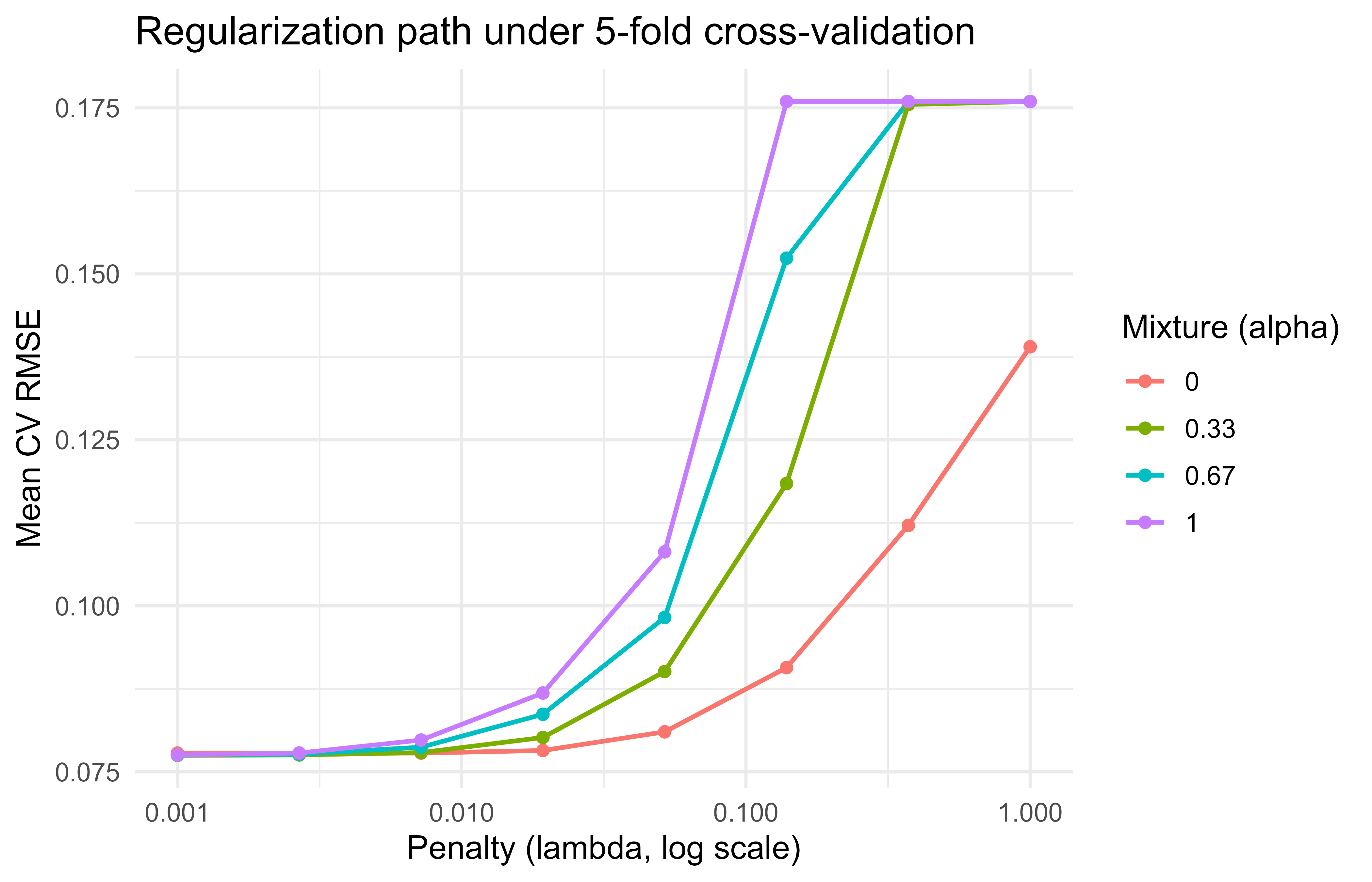
The table reports, for the five best hyperparameter settings, the mean cross-validated RMSE (mean) and its standard error across the five folds (std_err). Reading it, smaller penalty with a moderate mixture tends to win here, because the standardized predictors are already well behaved and need little shrinkage. The standard-error column is worth a glance too: when several top settings sit within one standard error of each other, they are practically tied, and you might reasonably prefer the simpler (more heavily penalized) one.
90.8.1 A figure from the tuning results
Figure 90.1 plots cross-validated RMSE against the penalty for each mixing value, which shows the characteristic U-shape of regularization: too little penalty overfits, too much underfits.
Figure 90.1: Cross-validated RMSE versus penalty across elastic-net mixtures on the Ames data.
90.8.2 Finalizing and evaluating once
Tuning told us which hyperparameters are best, but every number so far came from the training data’s folds. The honest verdict comes from the test set, which we have not touched since the split. Three functions close the loop. finalize_workflow() plugs the winning hyperparameters back into the workflow (replacing the tune() placeholders with concrete values), last_fit() trains on the full training set and scores the test set in a single leakage-safe call, and collect_metrics() returns the resulting test performance.
Warning
Call last_fit() exactly once, at the very end. If you peek at the test set, tune against it, and refit, you have turned your test set into another validation set and lost your one unbiased estimate of generalization.
Show code
.libPaths(c("C:/Users/miken/R/library-4.4", .libPaths()))best<-select_best(tuned, metric ="rmse")final_wf<-finalize_workflow(wf, best)final_fit<-last_fit(final_wf, split, metrics =metrics)collect_metrics(final_fit)#> # A tibble: 3 × 4#> .metric .estimator .estimate .config #> <chr> <chr> <dbl> <chr> #> 1 rmse standard 0.107 pre0_mod0_post0#> 2 rsq standard 0.659 pre0_mod0_post0#> 3 mae standard 0.0560 pre0_mod0_post0
The metrics here come from the test set, which was held out from splitting through tuning, so they are an unbiased estimate of generalization (on the log10 scale of sale price).
90.9 A from-scratch view of the leakage problem
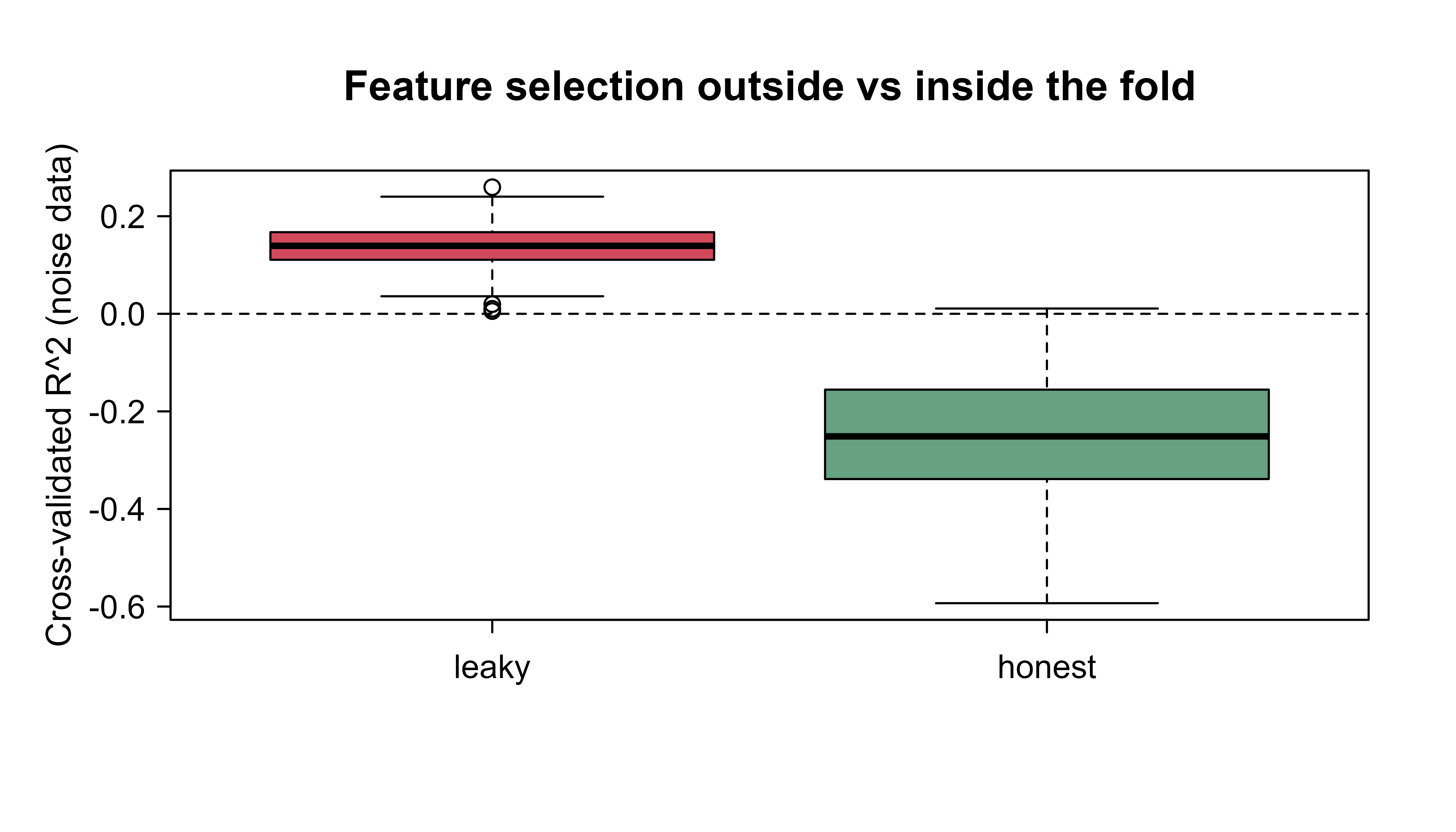
We have asserted several times that data-dependent steps must live inside each fold. This section proves it with numbers. The base-R simulation below contrasts two ways of doing a data-dependent step before cross-validation: the wrong way (do it once on all the data, then split) and the right way (redo it inside each fold). The trick that makes the lesson unmistakable is that the data is pure noise: the response is generated independently of every feature, so the true predictive \(R^2\) is zero. Any positive cross-validated \(R^2\) a method reports is therefore self-deception, and we can read leakage straight off the number.
The chunk includes two variants. The first standardizes (scaling, where leakage is real but mild) and the second selects the most correlated features (where leakage is dramatic, because selection peeks at the labels). Watching the gap between leaky and honest in each case shows why selection and encoding are far more dangerous than plain scaling. Figure 90.2 plots the result.
Show code
.libPaths(c("C:/Users/miken/R/library-4.4", .libPaths()))set.seed(1301)cv_r2<-function(X, y, folds, leak){n<-length(y)fold_id<-sample(rep(1:folds, length.out =n))if(leak){# WRONG: standardize using all rowsX<-scale(X)}preds<-numeric(n)for(fin1:folds){tr<-which(fold_id!=f)te<-which(fold_id==f)Xtr<-X[tr, , drop =FALSE]; Xte<-X[te, , drop =FALSE]if(!leak){# RIGHT: standardize using train rows onlymu<-colMeans(Xtr); sdv<-apply(Xtr, 2, sd)Xtr<-scale(Xtr, center =mu, scale =sdv)Xte<-scale(Xte, center =mu, scale =sdv)}df_tr<-data.frame(y =y[tr], Xtr)fit<-lm(y~., data =df_tr)preds[te]<-predict(fit, newdata =data.frame(Xte))}1-sum((y-preds)^2)/sum((y-mean(y))^2)}# Here leakage from scaling alone is mild; the larger lesson is that ANY# data-dependent step (selection, encoding) must live inside the fold.# We exaggerate by also selecting the most correlated noise features first.cv_r2_select<-function(X, y, folds, leak, keep=5){n<-length(y)fold_id<-sample(rep(1:folds, length.out =n))if(leak){# WRONG: pick features using all rowscors<-abs(cor(X, y))sel<-order(cors, decreasing =TRUE)[1:keep]X<-X[, sel, drop =FALSE]}preds<-numeric(n)for(fin1:folds){tr<-which(fold_id!=f); te<-which(fold_id==f)Xf<-Xif(!leak){# RIGHT: pick features using train rows onlycors<-abs(cor(X[tr, , drop =FALSE], y[tr]))sel<-order(cors, decreasing =TRUE)[1:keep]Xf<-X[, sel, drop =FALSE]}df_tr<-data.frame(y =y[tr], Xf[tr, , drop =FALSE])fit<-lm(y~., data =df_tr)preds[te]<-predict(fit, newdata =data.frame(Xf[te, , drop =FALSE]))}1-sum((y-preds)^2)/sum((y-mean(y))^2)}reps<-100res<-replicate(reps, {X<-matrix(rnorm(120*200), nrow =120)# n=120, p=200 noise featuresy<-rnorm(120)# target unrelated to Xc(leak =cv_r2_select(X, y, folds =5, leak =TRUE), honest =cv_r2_select(X, y, folds =5, leak =FALSE))})summary_tbl<-data.frame( approach =c("Select on all data (leaky)", "Select inside folds (honest)"), mean_cv_r2 =c(mean(res["leak", ]), mean(res["honest", ])))print(summary_tbl)#> approach mean_cv_r2#> 1 Select on all data (leaky) 0.1367566#> 2 Select inside folds (honest) -0.2523894boxplot(t(res), names =c("leaky", "honest"), ylab ="Cross-validated R^2 (noise data)", main ="Feature selection outside vs inside the fold", col =c("#d1495b", "#66a182"))abline(h =0, lty =2)
Figure 90.2: Cross-validated R-squared on pure-noise data, comparing feature selection done once on all rows against selection redone inside each fold.
The leaky version reports a healthy-looking positive cross-validated \(R^2\) even though the response is independent of every feature, purely because the feature selection peeked at the held-out rows. The honest version, which reselects inside each fold, hovers around (and often below) zero, which is the truth for noise. This is the whole argument for the framework in one picture: a tidymodels recipe placed inside tune_grid reproduces the honest behavior automatically, because any selection or estimation step it contains is refit per fold without you having to remember to do so.
Key idea
The danger of leakage is not that it makes a model fail loudly; it is that it makes a worthless model look good. The leaky curve in this experiment is the trap, and the only defense is to keep every data-dependent step inside the resampling loop.
90.10 Comparison with alternatives
tidymodels is not the only way to organize a modeling workflow, and it is worth knowing where it sits among the alternatives so you can choose deliberately. Table 90.3 sketches the main options, from rolling your own loops to the older caret framework, the more object-oriented mlr3 (covered in Chapter 91), and Python’s scikit-learn.
Table 90.3: How tidymodels compares with other ways to organize a modeling workflow, with the main strengths and weaknesses of each.
Many packages to learn, some overhead on tiny tasks
mlr3
Object-oriented, very flexible pipelines
Steeper learning curve, R6 style
Python scikit-learn
Huge ecosystem
Different language; less tidy data handling in R
The remaining sections cover two things you will want once a pipeline grows beyond a textbook example: making tuning faster, and turning a finished model into something you can deploy.
90.11 Scaling out the tuning grid
Because the (fold, candidate) fits in a grid search are independent of one another, they parallelize almost perfectly: each can run in its own R session. For large grids or large data, that is the easiest speedup available (the parallel computing chapter, Chapter 95, covers the backends in depth). The chunk below shows the idiomatic pattern with the future package. It is marked eval=FALSE because it depends on a parallel backend being registered and is specific to the machine it runs on, but it is correct code a reader can run as-is.
Show code
library(future)library(tune)# Use multiple local R sessions; tune detects the plan automatically.plan(multisession, workers =4)tuned_parallel<-tune_grid(wf, resamples =folds, grid =grid, metrics =metrics, control =control_grid(save_pred =TRUE, parallel_over ="everything"))plan(sequential)# reset
90.12 Racing to prune the grid
Parallelism makes each fit cheaper; racing makes you do fewer fits. Racing methods evaluate all candidates on a few folds first, run a statistical test to eliminate the candidates that are already clearly worse, and continue only with the survivors on the remaining folds. Because most candidates in a typical grid are mediocre, this often cuts tuning time by a large factor for the same final answer. The finetune package provides it. The code is correct and runnable but shown eval=FALSE to keep the book’s build fast.
Show code
library(finetune)tuned_race<-tune_race_anova(wf, resamples =folds, grid =30, # a space-filling design of 30 candidates metrics =metric_set(rmse), control =control_race(verbose_elim =TRUE))show_best(tuned_race, metric ="rmse")
90.13 Deploying a fitted workflow
The workflow’s habit of carrying its preprocessing inside one object pays off again at deployment. Because the fitted workflow already knows how to turn raw input columns into predictions, deploying it means little more than saving that object and calling predict() on new raw data, with no separate preprocessing script to keep in sync. Production tooling such as vetiver builds on exactly this, wrapping a fitted workflow as a versioned model behind a REST API. The snippet is eval=FALSE because vetiver and its server dependencies are outside the runnable set here, but it is current, idiomatic usage.
Show code
library(vetiver)library(plumber)fitted_wf<-extract_workflow(final_fit)# the trained recipe + modelv<-vetiver_model(fitted_wf, model_name ="ames_elastic_net")# Turn it into a REST APIpr()%>%vetiver_api(v)%>%pr_run(port =8080)
90.14 Practical guidance and pitfalls
The framework removes a great deal of room for error, but it cannot make every decision for you. The following checklist collects the habits that separate a trustworthy pipeline from a fragile one. Each is a place where the framework gives you the safe option but does not force it.
Split first, always. Call initial_split() before you look at any summary statistic that could influence a modeling choice. Treat the test set as sealed until the final last_fit().
Put every data-dependent step inside the recipe, not in a preprocessing script you run on the whole data set. This includes imputation means, scaling parameters, category collapsing, and especially target/effect encodings.
Match the resampling scheme to the data structure. Use grouped CV when rows cluster (multiple records per customer, repeated measures) and time-based resampling for anything with a temporal order, or you will leak the future into the past.
Order recipe steps deliberately: impute before normalizing, collapse rare levels (step_other) before step_dummy, and drop zero-variance columns (step_zv) after dummy creation since dummies can be all-zero in a fold.
Prefer space-filling grids or racing once you tune more than two hyperparameters; regular grids explode combinatorially.
Set seeds (set.seed) before splitting and resampling for reproducibility, and remember that parallel backends may need their own seeding controls.
Watch the metric you optimize. RMSE and MAE answer different questions, and for imbalanced classification, accuracy is misleading while ROC AUC, PR AUC, or log loss are usually better targets.
For tiny data sets the framework’s overhead can exceed a direct call; tidymodels shines as soon as you have multiple models, real preprocessing, or tuning.
Tip
If you remember only one rule from this chapter, make it this: anything that learns a number from the data goes inside the recipe, and the recipe goes inside the resampling loop. Almost every leakage bug is a violation of that one sentence.
90.14.1 When to use it
Reach for tidymodels whenever a project involves preprocessing that must be learned from data, comparison across several model families, hyperparameter tuning, or a need for reproducible, auditable pipelines that move cleanly to deployment. For a one-off lm() on clean data, base R is fine.
To recap the chapter in one breath: rsample splits and resamples, recipes declares preprocessing that is re-estimated per fold, parsnip specifies a model independently of its engine, workflows bundles the recipe and model so preprocessing always travels with the model, dials and tune search hyperparameters by resampling, and yardstick scores the result with the same code everywhere. The thread running through all of them is that data-dependent steps are estimated only on the rows a model is allowed to see, which is what turns a hopeful pipeline into an honest one.
90.15 Further reading
Kuhn and Johnson (2013), Applied Predictive Modeling. The conceptual backbone for resampling and preprocessing.
Kuhn and Silge (2022), Tidy Modeling with R. The definitive guide to the tidymodels packages, available free online.
Kuhn and Johnson (2019), Feature Engineering and Selection. Detailed treatment of recipe-style preprocessing and encodings.
Hastie, Tibshirani, and Friedman (2009), The Elements of Statistical Learning. Cross-validation, the bias-variance tradeoff, and the elastic net.
Zou and Hastie (2005), “Regularization and Variable Selection via the Elastic Net,” Journal of the Royal Statistical Society, Series B. Original elastic-net formulation.
Kuhn (2014) and the tune, recipes, and rsample package vignettes for current API details.
Leakage is any path by which information that would not be available at prediction time sneaks into training. It need not be dramatic. Standardizing the whole data set before splitting leaks the test rows’ mean and spread into the training features, and selecting “the most predictive variables” on all the data leaks the labels themselves.↩︎
You rarely call prep() and bake() by hand once a recipe lives inside a workflow; the framework calls them for you at the right moments. They are worth knowing because they are exactly where the leakage-safe behavior is enforced, and because calling them manually is the best way to inspect what a recipe actually produces.↩︎
Target encoding (also called effect or mean encoding) is a popular way to turn a high-cardinality category, say a ZIP code with hundreds of values, into a single numeric column. It is also one of the easiest places to leak, precisely because the encoded value is built from the response.↩︎
tidymodels deliberately says “analysis” and “assessment” rather than “train” and “test” for the pieces of a resample. The words keep the inner resampling loop verbally distinct from the one outer train/test split, which you touch only once at the very end.↩︎
A space-filling design asks: given that I can afford only, say, 30 candidates, where should I place them so that no large region of the space is left unexplored? The answer is not a grid, which wastes points on the corners, but a scatter chosen to keep candidates far apart.↩︎
We model log10(Sale_Price) rather than the price itself for the usual reasons: prices are right-skewed and multiplicative in spirit (a fixed percentage premium for an extra bedroom), so a log makes the relationship closer to linear and the error variance steadier. All reported errors are then on the log10 scale.↩︎
Source Code
# The tidymodels Framework {#sec-tidymodels-framework}```{r}#| include: falsesource("_common.R")``````{r tmf-setup, include=FALSE}knitr::opts_chunk$set(echo =TRUE, message =FALSE, warning =FALSE)```The `tidymodels` framework is a collection of R packages that share a common design for building predictive models. It plays the same role in R that `scikit-learn` pipelines play in Python: it gives you one consistent way to preprocess data, specify a model, resample, tune hyperparameters, and score predictions, regardless of which underlying engine (`glmnet`, `xgboost`, `ranger`, `keras`, and so on) actually does the fitting.This chapter treats `tidymodels` not as a single algorithm but as the plumbing that connects the algorithms in the rest of this book. The goal is to make the modeling workflow reproducible, leakage-free, and easy to swap parts in and out of.If you have spent any time fitting models in base R, you have probably felt the friction this framework removes. Every package speaks its own dialect: `glmnet` wants a matrix and calls its penalty `lambda`, `randomForest` wants a formula and calls its key knob `mtry`, and `xgboost` wants yet another input format. Worse, the safe handling of data (splitting before you compute anything, re-estimating preprocessing inside each resample) is left entirely to your discipline, and a single misplaced line can quietly invalidate every number you report. `tidymodels` exists to take both of those burdens off your shoulders: one vocabulary for all engines, and correct data handling by construction.::: {.callout-tip title="Intuition"}Think of `tidymodels` as an adapter layer. You describe *what* you want (standardize the predictors, fit an elastic net, tune the penalty by 5-fold cross-validation) and the framework handles *how* each underlying package wants to be called, and *when* each data-dependent quantity may be computed.:::By the end of the chapter you will be able to read and write a complete modeling pipeline: split the data once, declare preprocessing as a reusable object, specify a model independently of its engine, tune hyperparameters by resampling, and score the result honestly. We will also build a small from-scratch simulation that shows, in numbers, why the framework's "estimate inside every fold" rule is not pedantry but the difference between an honest error estimate and a self-deceiving one.## Where this fits in a modern ML workflowA predictive modeling project usually has the same skeleton no matter the algorithm:1. Split the data so that the test set never informs any modeling decision.2. Define preprocessing (imputation, encoding, scaling, feature creation).3. Choose a model and an engine.4. Estimate out-of-sample performance with resampling.5. Search over hyperparameters.6. Finalize and fit on the full training set, then evaluate once on the test set.Done by hand, each of these steps invites mistakes. The most common and most damaging is information leakage: computing a centering mean, a scaling standard deviation, or a category encoding on the full data set before splitting, so that knowledge of the held-out rows quietly enters the model.^[Leakage is any path by which information that would not be available at prediction time sneaks into training. It need not be dramatic. Standardizing the whole data set before splitting leaks the test rows' mean and spread into the training features, and selecting "the most predictive variables" on all the data leaks the labels themselves.]`tidymodels` is built so that every data-dependent transformation is *estimated on the analysis rows only* and then *applied* to the assessment rows. This is the single most important reason to use it.::: {.callout-important title="Key idea"}A modeling step is "data-dependent" if it learns a number from the data (a mean, a quantile, a set of retained categories, a PCA rotation). Every such number must be learned from training rows alone and then applied unchanged to held-out rows. The framework makes this the default rather than something you must remember.:::The framework breaks into focused packages, each owning one job in the skeleton above. @tbl-tidymodels-framework-package-map maps each package to its role and to the `scikit-learn` concept it most resembles, so readers coming from Python have a translation key.| Package | Job | Analogous concept ||---|---|---||`rsample`| Splits and resamples (CV, bootstrap, validation) | Train/test, `KFold`||`recipes`| Preprocessing as a reusable, fitted object |`ColumnTransformer` / `Pipeline` steps ||`parsnip`| Unified model specification across engines | Estimator interface ||`workflows`| Bundles a recipe and a model into one object |`Pipeline`||`dials`| Hyperparameter ranges and grids | Search space ||`tune`| Fits the workflow across the grid and resamples |`GridSearchCV`||`yardstick`| Metrics for regression and classification |`metrics` module ||`stacks`| Ensembles tuned candidates (@sec-model-stacking) | Stacking meta-learner |: The core tidymodels packages, the job each one owns in the modeling workflow, and the closest scikit-learn analogue. {#tbl-tidymodels-framework-package-map}The payoff is that you write the *intent* once. Changing from a penalized linear model to a boosted tree means editing the `parsnip` specification and leaving the recipe, resampling, and scoring code untouched.The rest of the chapter walks through these packages in the order you meet them in a real project: first the preprocessing object, then the model, then the bundle that joins them, then resampling, tuning, and scoring. We finish with one worked example that uses all of them together.## The preprocessing object: recipesA recipe is a description of how to turn raw columns into model-ready features. The single most important property of a recipe is that it separates the *definition* of a step from its *estimation*. You declare "center and scale all numeric predictors," and the actual means and standard deviations are learned later, only from the data you train on. A recipe is therefore more like a written instruction than a transformed data set: it is a plan that can be re-estimated on whatever rows you hand it.::: {.callout-tip title="Intuition"}A recipe is to your features what a cooking recipe is to a meal. Writing "add salt to taste" does not yet add any salt; the amount is decided when you actually cook, with the ingredients in front of you. Likewise `step_normalize()` does not yet subtract any mean; the mean is computed when the recipe is `prep()`ed on a specific set of training rows.:::Formally, suppose a numeric predictor $x$ is to be standardized. Standardization is the map$$z = \frac{x - \hat\mu}{\hat\sigma},$$where $\hat\mu$ and $\hat\sigma$ are the sample mean and standard deviation. The leakage-safe rule is that $\hat\mu$ and $\hat\sigma$ must be functions of the analysis (training) rows only:$$\hat\mu = \frac{1}{n_{\text{train}}} \sum_{i \in \text{train}} x_i,\qquad\hat\sigma^2 = \frac{1}{n_{\text{train}} - 1} \sum_{i \in \text{train}} (x_i - \hat\mu)^2 .$$The same fixed $\hat\mu, \hat\sigma$ are then applied to validation and test rows. `recipes` enforces this through two verbs: `prep()` estimates the quantities from training data, and `bake()` applies them to any data.^[You rarely call `prep()` and `bake()` by hand once a recipe lives inside a workflow; the framework calls them for you at the right moments. They are worth knowing because they are exactly where the leakage-safe behavior is enforced, and because calling them manually is the best way to inspect what a recipe actually produces.] When a recipe sits inside a workflow that is resampled, `prep()` is re-run inside every fold automatically, so each fold's preprocessing is estimated only on that fold's analysis rows.A recipe is built by chaining `step_*` functions, each one a named transformation. The steps you reach for most often fall into a few families. For missing data, the `step_impute_*` family fills gaps (by mean, median, $k$-nearest-neighbors, and so on). For categorical predictors, `step_other` collapses rare levels into a single "other" category and `step_dummy` turns categories into one-hot or contrast-coded columns. For numeric predictors, `step_normalize` centers and scales, while `step_zv` and `step_nzv` drop columns with zero or near-zero variance that carry no usable signal. For dimension reduction, `step_pca` replaces correlated predictors with a smaller set of components (see the dimension reduction chapter, @sec-dimension-reduction). The broader question of how to construct good features in the first place is the subject of the feature engineering chapter (@sec-feature-engineering).The order in which you add steps is itself a modeling decision, because each step sees the data as the previous steps left it.::: {.callout-warning}Impute before you scale, or the scaling statistics will be computed from incomplete columns. Collapse rare levels with `step_other` before `step_dummy`, or each rare level becomes its own near-empty dummy column. Drop zero-variance columns with `step_zv` after creating dummies, since a category present overall can be absent within a single fold and produce an all-zero dummy there.:::### Why estimation-then-application matters numericallyConsider a target encoding, where a categorical level is replaced by the mean response in that level.^[Target encoding (also called effect or mean encoding) is a popular way to turn a high-cardinality category, say a ZIP code with hundreds of values, into a single numeric column. It is also one of the easiest places to leak, precisely because the encoded value is built from the response.] If the encoding is computed on all rows, the encoded value for a row literally contains that row's own response, and cross-validated error becomes optimistic. Estimating the encoding inside each fold removes the row's own contribution from its features and gives an honest error estimate. The recipe interface makes the correct behavior the default rather than something you must remember to code.::: {.callout-tip title="When to use this"}Whenever a preprocessing step learns anything from the data (an imputation value, a scaling constant, a retained category set, a PCA rotation, an encoding), put it in a recipe rather than running it once on the whole data set. The recipe is the mechanism that guarantees the step is re-estimated per fold.:::## The model specification: parsnipA `parsnip` specification decouples three things that base R functions tangle together: the model type (what family of model, say linear regression or a random forest), the computational engine (which package actually fits it, say `glmnet` or `lm`), and the mode (regression or classification). Separating these means you can change one without touching the others, swapping `glmnet` for `keras` without rewriting your argument names. A specification reads almost like a sentence:```{r tmf-parsnip-demo, eval=TRUE}.libPaths(c("C:/Users/miken/R/library-4.4", .libPaths()))library(parsnip)spec <-linear_reg(penalty =0.01, mixture =1) %>%set_engine("glmnet") %>%set_mode("regression")spec```Here `linear_reg` is the model, `glmnet` is the engine, and the arguments `penalty` and `mixture` are *engine-agnostic names*. `penalty` is the total regularization strength $\lambda$ and `mixture` is the elastic-net mixing parameter $\alpha$ in the penalized objective$$\hat\beta = \arg\min_{\beta} \; \frac{1}{2n}\sum_{i=1}^{n}\bigl(y_i - x_i^\top \beta\bigr)^2\; + \; \lambda \Bigl[ \alpha \lVert \beta \rVert_1 + \tfrac{1}{2}(1-\alpha)\lVert \beta \rVert_2^2 \Bigr].$$`mixture = 1` is the lasso, `mixture = 0` is ridge, and values in between give the elastic net. The point of `parsnip` is that these same two argument names map to whatever the chosen engine calls them internally, so you do not memorize each package's argument conventions.::: {.callout-tip}Notice that printing a specification does not fit anything; it only shows the plan. A `parsnip` object is fit later, either directly with `fit()` or, more commonly, by placing it in a workflow. Building specifications without fitting them is cheap, which makes it easy to define several model families side by side and compare them on the same resamples.:::To mark an argument for tuning rather than fixing it, you write `tune()` as a placeholder in place of a value. This says "do not pick a number yet; treat this as something to search over." Later, `dials` supplies a sensible range for that argument and `tune` fills in the candidate values. We will see exactly this pattern in the worked example, where both `penalty` and `mixture` are left as `tune()`.## Bundling with workflowsSo far we have a recipe (the preprocessing plan) and a specification (the model plan) as two separate objects. A workflow joins them into one. It is a container holding exactly one preprocessor and one model, and treating the pair as a single unit is what keeps training and prediction in step.Fitting the workflow fits the recipe and the model together; predicting on new data automatically bakes the recipe before calling the model. This guarantees that training and prediction use identical preprocessing, which is the second most common source of bugs after leakage.::: {.callout-note}A common base-R bug is to scale the training data, fit a model, then forget to apply the *same* scaling to new data at prediction time, or to recompute it from the new data. A workflow makes that mistake structurally impossible: the preprocessing travels with the model inside one object.:::```{r tmf-workflow-shape, eval=TRUE}.libPaths(c("C:/Users/miken/R/library-4.4", .libPaths()))library(workflows)library(recipes)library(parsnip)rec <-recipe(mpg ~ ., data = mtcars) %>%step_normalize(all_numeric_predictors())wf <-workflow() %>%add_recipe(rec) %>%add_model(linear_reg() %>%set_engine("lm"))wf```## Resampling: rsampleWith a fitted workflow in hand, the next question is how well it will do on data it has not seen. We cannot answer that by scoring on the training data, since a flexible model can memorize its training rows and look better than it is. Resampling answers it honestly by repeatedly holding out part of the training data, fitting on the rest, and scoring on the part held out.The workhorse is $V$-fold cross-validation. The training rows are partitioned into $V$ folds. For fold $v$, the model is fit on the other $V-1$ folds (the *analysis* set) and scored on fold $v$ (the *assessment* set).^[`tidymodels` deliberately says "analysis" and "assessment" rather than "train" and "test" for the pieces of a resample. The words keep the inner resampling loop verbally distinct from the one outer train/test split, which you touch only once at the very end.] The cross-validated estimate of a metric $L$ is$$\widehat{\text{CV}} = \frac{1}{V} \sum_{v=1}^{V} L\bigl(y_{(v)},\, \hat f_{-v}(x_{(v)})\bigr),$$where $\hat f_{-v}$ is the model fit without fold $v$. Its standard error across folds gives a rough sense of how stable the estimate is. `rsample` produces the fold structure as a table of row indices, never copying the data, and stores analysis/assessment splits that the rest of the framework consumes.The choice of resampling scheme is itself a bias-variance tradeoff: a single split is cheap but its estimate jumps around depending on which rows landed in the validation set, while many folds average out that noise at a higher computational cost. @tbl-tidymodels-framework-resampling-schemes summarizes the usual options and when each one earns its keep.::: {.callout-tip}When in doubt, 10-fold cross-validation is the sensible default for most tabular problems. Reach for the other schemes only when the data structure demands it: grouped CV when rows cluster, time-based resampling when rows are ordered in time.:::| Scheme | What it does | Bias | Variance | When to use ||---|---|---|---|---|| Validation split | One train/validation cut | Higher | Lower | Very large data, fast iteration || 5- or 10-fold CV | Average over $V$ folds | Low | Moderate | Default for most problems || Repeated CV | CV repeated $r$ times | Low | Lower than single CV | Small data, need stable estimates || Bootstrap | Sample with replacement | Optimistic-ish | Low | Uncertainty of statistics, small data || Grouped CV | Folds respect a grouping id | Low | Moderate | Repeated measures, leakage across groups || Time-based | Rolling/expanding windows | Low | Moderate | Temporal data, no future leakage |: Common resampling schemes in rsample, their bias and variance behavior, and the situations where each is the right choice. {#tbl-tidymodels-framework-resampling-schemes}## Tuning: dials and tuneHyperparameter tuning searches a space of model settings to minimize a resampled metric. Let $\theta$ denote the hyperparameters (for elastic net, $\theta = (\lambda, \alpha)$). The objective is$$\theta^\star = \arg\min_{\theta \in \Theta} \; \widehat{\text{CV}}(\theta),$$estimated by fitting the workflow on every (fold, candidate) pair. Two packages divide the labor: `dials` defines the search space $\Theta$ and builds the grid of candidates, while `tune` orchestrates the fitting across all folds and collects the metrics.The size of the grid is where tuning gets expensive. A regular grid over $d$ parameters with $k$ levels each costs $k^d$ candidates, and that product grows alarmingly: three parameters at five levels is already $125$ settings, each fit $V$ times. Space-filling designs (Latin hypercube, max-entropy) spread a fixed budget of candidates evenly through the space instead of on a rigid lattice, and they are the better choice once $d$ is more than two.^[A space-filling design asks: given that I can afford only, say, 30 candidates, where should I place them so that no large region of the space is left unexplored? The answer is not a grid, which wastes points on the corners, but a scatter chosen to keep candidates far apart.] For an even larger saving, the `finetune` package offers racing, which evaluates all candidates on a few folds, eliminates the clear losers early, and continues only with the survivors, and simulated annealing for guided search.::: {.callout-warning}Tuning multiplies cost by both the grid size and the number of folds. A 100-candidate grid under 10-fold CV is 1000 model fits. Before launching a large search, sanity-check the arithmetic, and consider racing or a space-filling design to keep it tractable.:::## Scoring: yardstick`yardstick` provides metrics with a consistent interface and lets you bundle several into a metric set. For regression the common choices are root mean squared error,$$\text{RMSE} = \sqrt{\frac{1}{n}\sum_{i=1}^{n}(y_i - \hat y_i)^2},$$mean absolute error, and the coefficient of determination $R^2$. For classification you get accuracy, the area under the ROC curve, log loss, and the Brier score, among others. Because metrics are ordinary functions of a data frame of predictions, the same code path scores resamples, tuning candidates, and the final test set, so a metric set you define once is reused everywhere.::: {.callout-warning}The metric you optimize is a modeling choice, not a formality. RMSE and MAE answer different questions (RMSE punishes large errors harder), and for imbalanced classification, accuracy is actively misleading: a model that always predicts the majority class can score 95% accuracy while being useless. Prefer ROC AUC, PR AUC, or log loss there.:::## A full pipeline: cross-validated tuning on Ames housingWe have now met every package on its own. This section puts them together in one end-to-end pipeline so you can see how the pieces lock into place. The demonstration is verified to execute: a recipe, a tunable elastic-net workflow, 5-fold cross-validation, a grid search, and a tuned-metrics table. The data is the Ames housing set restricted to a few predictors, with a log-transformed sale price.^[We model `log10(Sale_Price)` rather than the price itself for the usual reasons: prices are right-skewed and multiplicative in spirit (a fixed percentage premium for an extra bedroom), so a log makes the relationship closer to linear and the error variance steadier. All reported errors are then on the log10 scale.] Read the comments in the chunk as the table of contents for the whole framework: each numbered block is one of the six steps from the skeleton at the start of the chapter.```{r tmf-full-demo, eval=TRUE}.libPaths(c("C:/Users/miken/R/library-4.4", .libPaths()))suppressPackageStartupMessages({library(recipes)library(parsnip)library(workflows)library(rsample)library(tune)library(dials)library(yardstick)library(dplyr)library(ggplot2)})set.seed(1301)data(ames, package ="modeldata")dat <- ames %>%transmute(Sale_Price =log10(Sale_Price),Gr_Liv_Area = Gr_Liv_Area,Year_Built = Year_Built,Total_Bsmt_SF = Total_Bsmt_SF,Lot_Area = Lot_Area,Neighborhood = Neighborhood,Bldg_Type = Bldg_Type )# 1. Split, leaving the test set untouched until the very end.split <-initial_split(dat, prop =0.8)train <-training(split)test <-testing(split)# 2. Resampling scheme estimated only on training rows.folds <-vfold_cv(train, v =5)# 3. Recipe: collapse rare neighborhoods, dummy-encode, drop dead columns,# and standardize. Every quantity is learned per-fold.rec <-recipe(Sale_Price ~ ., data = train) %>%step_other(Neighborhood, threshold =0.05) %>%step_dummy(all_nominal_predictors()) %>%step_zv(all_predictors()) %>%step_normalize(all_numeric_predictors())# 4. Tunable elastic-net specification.en_spec <-linear_reg(penalty =tune(), mixture =tune()) %>%set_engine("glmnet") %>%set_mode("regression")wf <-workflow() %>%add_recipe(rec) %>%add_model(en_spec)# 5. Search space and grid.grid <-grid_regular(penalty(range =c(-3, 0)), # log10 scale: 1e-3 to 1e0mixture(range =c(0, 1)),levels =c(penalty =8, mixture =4))# 6. Cross-validated tuning.metrics <-metric_set(rmse, rsq, mae)tuned <-tune_grid( wf,resamples = folds,grid = grid,metrics = metrics)# Tuned metrics table: best candidates by RMSE.top_rmse <-show_best(tuned, metric ="rmse", n =5)print(top_rmse)```The table reports, for the five best hyperparameter settings, the mean cross-validated RMSE (`mean`) and its standard error across the five folds (`std_err`). Reading it, smaller `penalty` with a moderate `mixture` tends to win here, because the standardized predictors are already well behaved and need little shrinkage. The standard-error column is worth a glance too: when several top settings sit within one standard error of each other, they are practically tied, and you might reasonably prefer the simpler (more heavily penalized) one.### A figure from the tuning results@fig-tidymodels-framework-tune-path plots cross-validated RMSE against the penalty for each mixing value, which shows the characteristic U-shape of regularization: too little penalty overfits, too much underfits.```{r fig-tidymodels-framework-tune-path, eval=TRUE, fig.cap="Cross-validated RMSE versus penalty across elastic-net mixtures on the Ames data.", fig.width=7, fig.height=4.5}.libPaths(c("C:/Users/miken/R/library-4.4", .libPaths()))cv_results <-collect_metrics(tuned) %>% dplyr::filter(.metric =="rmse")ggplot(cv_results,aes(x = penalty, y = mean,color =factor(round(mixture, 2)),group =factor(round(mixture, 2)))) +geom_line() +geom_point(size =1.6) +scale_x_log10() +labs(x ="Penalty (lambda, log scale)",y ="Mean CV RMSE",color ="Mixture (alpha)",title ="Regularization path under 5-fold cross-validation" ) +theme_minimal(base_size =12)```### Finalizing and evaluating onceTuning told us which hyperparameters are best, but every number so far came from the training data's folds. The honest verdict comes from the test set, which we have not touched since the split. Three functions close the loop. `finalize_workflow()` plugs the winning hyperparameters back into the workflow (replacing the `tune()` placeholders with concrete values), `last_fit()` trains on the full training set and scores the test set in a single leakage-safe call, and `collect_metrics()` returns the resulting test performance.::: {.callout-warning}Call `last_fit()` exactly once, at the very end. If you peek at the test set, tune against it, and refit, you have turned your test set into another validation set and lost your one unbiased estimate of generalization.:::```{r tmf-finalize, eval=TRUE}.libPaths(c("C:/Users/miken/R/library-4.4", .libPaths()))best <-select_best(tuned, metric ="rmse")final_wf <-finalize_workflow(wf, best)final_fit <-last_fit(final_wf, split, metrics = metrics)collect_metrics(final_fit)```The metrics here come from the test set, which was held out from splitting through tuning, so they are an unbiased estimate of generalization (on the log10 scale of sale price).## A from-scratch view of the leakage problemWe have asserted several times that data-dependent steps must live inside each fold. This section proves it with numbers. The base-R simulation below contrasts two ways of doing a data-dependent step before cross-validation: the wrong way (do it once on all the data, then split) and the right way (redo it inside each fold). The trick that makes the lesson unmistakable is that the data is pure noise: the response is generated independently of every feature, so the true predictive $R^2$ is zero. Any positive cross-validated $R^2$ a method reports is therefore self-deception, and we can read leakage straight off the number.The chunk includes two variants. The first standardizes (scaling, where leakage is real but mild) and the second selects the most correlated features (where leakage is dramatic, because selection peeks at the labels). Watching the gap between leaky and honest in each case shows why selection and encoding are far more dangerous than plain scaling. @fig-tidymodels-framework-leakage-sim plots the result.```{r fig-tidymodels-framework-leakage-sim, eval=TRUE, fig.cap="Cross-validated R-squared on pure-noise data, comparing feature selection done once on all rows against selection redone inside each fold.", fig.width=7, fig.height=4}.libPaths(c("C:/Users/miken/R/library-4.4", .libPaths()))set.seed(1301)cv_r2 <-function(X, y, folds, leak) { n <-length(y) fold_id <-sample(rep(1:folds, length.out = n))if (leak) { # WRONG: standardize using all rows X <-scale(X) } preds <-numeric(n)for (f in1:folds) { tr <-which(fold_id != f) te <-which(fold_id == f) Xtr <- X[tr, , drop =FALSE]; Xte <- X[te, , drop =FALSE]if (!leak) { # RIGHT: standardize using train rows only mu <-colMeans(Xtr); sdv <-apply(Xtr, 2, sd) Xtr <-scale(Xtr, center = mu, scale = sdv) Xte <-scale(Xte, center = mu, scale = sdv) } df_tr <-data.frame(y = y[tr], Xtr) fit <-lm(y ~ ., data = df_tr) preds[te] <-predict(fit, newdata =data.frame(Xte)) }1-sum((y - preds)^2) /sum((y -mean(y))^2)}# Here leakage from scaling alone is mild; the larger lesson is that ANY# data-dependent step (selection, encoding) must live inside the fold.# We exaggerate by also selecting the most correlated noise features first.cv_r2_select <-function(X, y, folds, leak, keep =5) { n <-length(y) fold_id <-sample(rep(1:folds, length.out = n))if (leak) { # WRONG: pick features using all rows cors <-abs(cor(X, y)) sel <-order(cors, decreasing =TRUE)[1:keep] X <- X[, sel, drop =FALSE] } preds <-numeric(n)for (f in1:folds) { tr <-which(fold_id != f); te <-which(fold_id == f) Xf <- Xif (!leak) { # RIGHT: pick features using train rows only cors <-abs(cor(X[tr, , drop =FALSE], y[tr])) sel <-order(cors, decreasing =TRUE)[1:keep] Xf <- X[, sel, drop =FALSE] } df_tr <-data.frame(y = y[tr], Xf[tr, , drop =FALSE]) fit <-lm(y ~ ., data = df_tr) preds[te] <-predict(fit, newdata =data.frame(Xf[te, , drop =FALSE])) }1-sum((y - preds)^2) /sum((y -mean(y))^2)}reps <-100res <-replicate(reps, { X <-matrix(rnorm(120*200), nrow =120) # n=120, p=200 noise features y <-rnorm(120) # target unrelated to Xc(leak =cv_r2_select(X, y, folds =5, leak =TRUE),honest =cv_r2_select(X, y, folds =5, leak =FALSE))})summary_tbl <-data.frame(approach =c("Select on all data (leaky)", "Select inside folds (honest)"),mean_cv_r2 =c(mean(res["leak", ]), mean(res["honest", ])))print(summary_tbl)boxplot(t(res),names =c("leaky", "honest"),ylab ="Cross-validated R^2 (noise data)",main ="Feature selection outside vs inside the fold",col =c("#d1495b", "#66a182"))abline(h =0, lty =2)```The leaky version reports a healthy-looking positive cross-validated $R^2$ even though the response is independent of every feature, purely because the feature selection peeked at the held-out rows. The honest version, which reselects inside each fold, hovers around (and often below) zero, which is the truth for noise. This is the whole argument for the framework in one picture: a `tidymodels` recipe placed inside `tune_grid` reproduces the honest behavior automatically, because any selection or estimation step it contains is refit per fold without you having to remember to do so.::: {.callout-important title="Key idea"}The danger of leakage is not that it makes a model fail loudly; it is that it makes a worthless model look good. The leaky curve in this experiment is the trap, and the only defense is to keep every data-dependent step inside the resampling loop.:::## Comparison with alternatives`tidymodels` is not the only way to organize a modeling workflow, and it is worth knowing where it sits among the alternatives so you can choose deliberately. @tbl-tidymodels-framework-alternatives sketches the main options, from rolling your own loops to the older `caret` framework, the more object-oriented `mlr3` (covered in @sec-mlr3-ecosystem), and Python's `scikit-learn`.| Approach | Pros | Cons ||---|---|---|| Hand-written loops + base R | Full control, no dependencies | Easy to leak, verbose, hard to swap models ||`caret` (older R framework) | Mature, many models | Monolithic, harder to extend, less composable ||`tidymodels`| Composable, leakage-safe, engine-agnostic, tidy output | Many packages to learn, some overhead on tiny tasks ||`mlr3`| Object-oriented, very flexible pipelines | Steeper learning curve, R6 style || Python `scikit-learn`| Huge ecosystem | Different language; less tidy data handling in R |: How tidymodels compares with other ways to organize a modeling workflow, with the main strengths and weaknesses of each. {#tbl-tidymodels-framework-alternatives}The remaining sections cover two things you will want once a pipeline grows beyond a textbook example: making tuning faster, and turning a finished model into something you can deploy.## Scaling out the tuning gridBecause the (fold, candidate) fits in a grid search are independent of one another, they parallelize almost perfectly: each can run in its own R session. For large grids or large data, that is the easiest speedup available (the parallel computing chapter, @sec-parallel-computing, covers the backends in depth). The chunk below shows the idiomatic pattern with the `future` package. It is marked `eval=FALSE` because it depends on a parallel backend being registered and is specific to the machine it runs on, but it is correct code a reader can run as-is.```{r tmf-parallel, eval=FALSE}library(future)library(tune)# Use multiple local R sessions; tune detects the plan automatically.plan(multisession, workers =4)tuned_parallel <-tune_grid( wf,resamples = folds,grid = grid,metrics = metrics,control =control_grid(save_pred =TRUE, parallel_over ="everything"))plan(sequential) # reset```## Racing to prune the gridParallelism makes each fit cheaper; racing makes you do fewer fits. Racing methods evaluate all candidates on a few folds first, run a statistical test to eliminate the candidates that are already clearly worse, and continue only with the survivors on the remaining folds. Because most candidates in a typical grid are mediocre, this often cuts tuning time by a large factor for the same final answer. The `finetune` package provides it. The code is correct and runnable but shown `eval=FALSE` to keep the book's build fast.```{r tmf-racing, eval=FALSE}library(finetune)tuned_race <-tune_race_anova( wf,resamples = folds,grid =30, # a space-filling design of 30 candidatesmetrics =metric_set(rmse),control =control_race(verbose_elim =TRUE))show_best(tuned_race, metric ="rmse")```## Deploying a fitted workflowThe workflow's habit of carrying its preprocessing inside one object pays off again at deployment. Because the fitted workflow already knows how to turn raw input columns into predictions, deploying it means little more than saving that object and calling `predict()` on new raw data, with no separate preprocessing script to keep in sync. Production tooling such as `vetiver` builds on exactly this, wrapping a fitted workflow as a versioned model behind a REST API. The snippet is `eval=FALSE` because `vetiver` and its server dependencies are outside the runnable set here, but it is current, idiomatic usage.```{r tmf-vetiver, eval=FALSE}library(vetiver)library(plumber)fitted_wf <-extract_workflow(final_fit) # the trained recipe + modelv <-vetiver_model(fitted_wf, model_name ="ames_elastic_net")# Turn it into a REST APIpr() %>%vetiver_api(v) %>%pr_run(port =8080)```## Practical guidance and pitfallsThe framework removes a great deal of room for error, but it cannot make every decision for you. The following checklist collects the habits that separate a trustworthy pipeline from a fragile one. Each is a place where the framework gives you the safe option but does not force it.- Split first, always. Call `initial_split()` before you look at any summary statistic that could influence a modeling choice. Treat the test set as sealed until the final `last_fit()`.- Put every data-dependent step inside the recipe, not in a preprocessing script you run on the whole data set. This includes imputation means, scaling parameters, category collapsing, and especially target/effect encodings.- Match the resampling scheme to the data structure. Use grouped CV when rows cluster (multiple records per customer, repeated measures) and time-based resampling for anything with a temporal order, or you will leak the future into the past.- Order recipe steps deliberately: impute before normalizing, collapse rare levels (`step_other`) before `step_dummy`, and drop zero-variance columns (`step_zv`) after dummy creation since dummies can be all-zero in a fold.- Prefer space-filling grids or racing once you tune more than two hyperparameters; regular grids explode combinatorially.- Set seeds (`set.seed`) before splitting and resampling for reproducibility, and remember that parallel backends may need their own seeding controls.- Watch the metric you optimize. RMSE and MAE answer different questions, and for imbalanced classification, accuracy is misleading while ROC AUC, PR AUC, or log loss are usually better targets.- For tiny data sets the framework's overhead can exceed a direct call; `tidymodels` shines as soon as you have multiple models, real preprocessing, or tuning.::: {.callout-tip}If you remember only one rule from this chapter, make it this: anything that learns a number from the data goes inside the recipe, and the recipe goes inside the resampling loop. Almost every leakage bug is a violation of that one sentence.:::### When to use itReach for `tidymodels` whenever a project involves preprocessing that must be learned from data, comparison across several model families, hyperparameter tuning, or a need for reproducible, auditable pipelines that move cleanly to deployment. For a one-off `lm()` on clean data, base R is fine.To recap the chapter in one breath: `rsample` splits and resamples, `recipes` declares preprocessing that is re-estimated per fold, `parsnip` specifies a model independently of its engine, `workflows` bundles the recipe and model so preprocessing always travels with the model, `dials` and `tune` search hyperparameters by resampling, and `yardstick` scores the result with the same code everywhere. The thread running through all of them is that data-dependent steps are estimated only on the rows a model is allowed to see, which is what turns a hopeful pipeline into an honest one.## Further reading- Kuhn and Johnson (2013), *Applied Predictive Modeling*. The conceptual backbone for resampling and preprocessing.- Kuhn and Silge (2022), *Tidy Modeling with R*. The definitive guide to the `tidymodels` packages, available free online.- Kuhn and Johnson (2019), *Feature Engineering and Selection*. Detailed treatment of recipe-style preprocessing and encodings.- Hastie, Tibshirani, and Friedman (2009), *The Elements of Statistical Learning*. Cross-validation, the bias-variance tradeoff, and the elastic net.- Zou and Hastie (2005), "Regularization and Variable Selection via the Elastic Net," *Journal of the Royal Statistical Society, Series B*. Original elastic-net formulation.- Kuhn (2014) and the `tune`, `recipes`, and `rsample` package vignettes for current API details.