Suppose you are dropped into an unfamiliar building and told there is an exit somewhere, with a small reward waiting outside. Nobody hands you a floor plan. You can only walk around, occasionally bump into a wall, and eventually stumble out the door. Do this many times and something useful happens: you start to sense which corridors lead somewhere good and which dead-end, long before you can articulate the building’s layout. You learn to act well without ever writing down a map.
That is the situation this chapter studies. In the language of Markov decision processes, the “map” is the transition model (where each action takes you) together with the reward function (what each move pays). When you know both, you can solve for the optimal behavior by dynamic programming: value iteration and policy iteration sweep through the known dynamics and compute the best policy directly (see the foundations of reinforcement learning chapter, Chapter 64). But in most real problems the dynamics are unknown. A robot does not know in advance how its motors interact with a slippery floor; a recommendation agent does not know how a user will react to a new layout. The agent has to learn purely from experience, one transition at a time. This is the model-free setting, and it is where Monte Carlo and temporal-difference (TD) methods live.
The two ideas in the title sit at opposite ends of a spectrum. Monte Carlo methods wait until an episode finishes and then learn from the total reward actually collected: honest but patient. Temporal-difference methods update after every single step, using their own current guess of the future as a stand-in for the rest of the episode: a guess that bootstraps off another guess. That sounds circular, and the surprising fact, made precise below, is that it works, often far better than waiting. By the end of the chapter you will understand the TD update and the TD error, see why SARSA and Q-learning differ by a single symbol yet behave differently near danger, and have a runnable base-R agent that learns to walk along a cliff without falling off.
Note
This chapter assumes you have met the Markov decision process (MDP) and the Bellman equations, for instance through value iteration on a known model. Here the model is unknown. Everything is learned from sampled experience: tuples of state, action, reward, and next state.
66.1 Notation and the prediction problem
We work with a finite MDP. At each time step \(t\) the agent is in a state \(S_t \in \mathcal{S}\), takes an action \(A_t \in \mathcal{A}\), receives a scalar reward \(R_{t+1} \in \mathbb{R}\), and moves to a new state \(S_{t+1}\). A policy\(\pi(a \mid s)\) gives the probability of choosing action \(a\) in state \(s\). The agent’s goal is to maximize the expected return, the discounted sum of future rewards
where the discount factor\(\gamma \in [0,1]\) trades off immediate against later reward. A value of \(\gamma\) near \(0\) makes the agent myopic; near \(1\) it cares about the distant future.
Two value functions summarize how good things are under a policy \(\pi\):
The state-value\(v_\pi(s)\) is the expected return from \(s\) onward; the action-value\(q_\pi(s,a)\) is the expected return after committing to action \(a\) in \(s\) and following \(\pi\) afterward. Because the model is unknown, action-values are the more useful object: if you know \(q\), you can act greedily by picking \(\arg\max_a q(s,a)\) without ever consulting a transition model. Learning \(v_\pi\) or \(q_\pi\) for a fixed \(\pi\) is the prediction problem; improving \(\pi\) toward the optimal policy \(\pi_*\) is the control problem.
Key idea
When the dynamics are unknown, action-values \(q(s,a)\) are worth more than state-values \(v(s)\), because choosing the best action from \(q\) needs no model, whereas choosing from \(v\) requires knowing where each action would take you.
66.1.1 The Bellman operator and its fixed point
All the convergence results in this chapter rest on a single structural fact: the value function is the unique fixed point of a contraction mapping. Making this precise pays off later, because every algorithm here is a sampled, stochastic version of applying that mapping.
Conditioning the return identity \(G_t = R_{t+1} + \gamma G_{t+1}\) on \(S_t = s\) and taking expectations under \(\pi\) gives the Bellman expectation equation
\[
v_\pi(s) \;=\; \sum_{a} \pi(a \mid s) \sum_{s', r} p(s', r \mid s, a)\,\bigl[\, r + \gamma\, v_\pi(s') \,\bigr],
\tag{66.1}\]
where \(p(s', r \mid s, a)\) is the (unknown) joint transition-reward kernel. Collect the values into a vector \(v \in \mathbb{R}^{|\mathcal{S}|}\) and define the Bellman expectation operator\(T^\pi : \mathbb{R}^{|\mathcal{S}|} \to \mathbb{R}^{|\mathcal{S}|}\) componentwise by
with \(r_\pi(s) = \mathbb{E}_\pi[R_{t+1} \mid S_t = s]\) the expected one-step reward and \(P_\pi\) the state-to-state transition matrix induced by \(\pi\). Equation Equation 66.1 says exactly that \(v_\pi\) satisfies \(T^\pi v_\pi = v_\pi\), i.e. \(v_\pi\) is a fixed point of \(T^\pi\).
This fixed point is unique and globally attracting because \(T^\pi\) is a \(\gamma\)-contraction in the sup-norm. For any two value vectors \(u, w\),
where the last equality uses \(\|P_\pi\|_\infty = 1\) because each row of \(P_\pi\) is a probability distribution and therefore sums to one with nonnegative entries. For \(\gamma < 1\) this is a strict contraction, so by the Banach fixed-point theorem \(T^\pi\) has a unique fixed point and the iteration \(v_{k+1} = T^\pi v_k\) converges geometrically, \(\|v_k - v_\pi\|_\infty \le \gamma^k \|v_0 - v_\pi\|_\infty\), from any start \(v_0\). The action-value analogue \(q_\pi = T^\pi q_\pi\) and the optimal-value operator \((T^* v)(s) = \max_a \mathbb{E}[R_{t+1} + \gamma v(S_{t+1}) \mid s, a]\) are contractions by the same argument (the \(\max\) is nonexpansive), giving the optimal value functions \(v_*, q_*\) as their fixed points. TD(0) replaces the expectation in \(T^\pi\) with a single sample, and Q-learning replaces the expectation in \(T^*\) with a single sample; that is the entire conceptual content of both algorithms.
Note
The contraction is in the weighted or sup norm, not in Euclidean norm. This distinction is harmless in the tabular case but becomes the crux of stability once linear function approximation enters: \(T^\pi\) is a contraction in the \(\mu_\pi\)-weighted norm (with \(\mu_\pi\) the stationary distribution) for on-policy sampling, which is why on-policy TD with linear features converges while off-policy TD need not.
66.2 Monte Carlo: learn from complete returns
The most direct way to estimate \(v_\pi(s)\) is to take its definition literally. Run the policy, record the return that actually followed each visit to \(s\), and average those returns. By the law of large numbers the average converges to the expectation. This is the Monte Carlo (MC) idea, and it requires only the ability to sample episodes, not any knowledge of transition probabilities.
Concretely, suppose state \(s\) was visited and the episode that followed yielded return \(G\). The every-visit MC estimate maintains a running average
where \(\alpha\) is a step size (using \(\alpha = 1/N(s)\), with \(N(s)\) the visit count, recovers the exact sample mean). The quantity \(G - V(s)\) is the error between the realized return and the current estimate, and we nudge \(V(s)\) a fraction of the way toward \(G\).
The defining feature, and the catch, is that \(G\) is only known once the episode terminates. Monte Carlo cannot learn from an unfinished episode, and it cannot be used at all in a setting that never ends. It is also high variance: a single episode’s return depends on every random action and transition along the way, so estimates wobble.1
Intuition
Monte Carlo is like grading a chess move only by who won the game. Correct on average, but you must play to the end, and a single blunder elsewhere can wrongly tar a good move.
66.3 Temporal-difference learning: bootstrap from the next step
Temporal-difference learning keeps the averaging idea but refuses to wait. The insight is that the return obeys a recursive relationship, the Bellman equation: \(G_t = R_{t+1} + \gamma G_{t+1}\). We cannot observe \(G_{t+1}\), but we already maintain an estimate of its expectation, namely \(V(S_{t+1})\). So we substitute the estimate for the unknown and update immediately after one step. This is the TD(0) update:
The bracketed quantity \(\delta_t\) is the TD error. It compares two estimates of the same thing: the one-step target\(R_{t+1} + \gamma V(S_{t+1})\), which mixes a real observed reward with a bootstrapped guess of the rest, against the current estimate \(V(S_t)\). If the target exceeds the estimate, \(S_t\) was better than we thought and we raise its value; if lower, we lower it.
Key idea
The TD error \(\delta_t = R_{t+1} + \gamma V(S_{t+1}) - V(S_t)\) is the engine of reinforcement learning. It measures surprise: the gap between what you expected and what one real step plus your own forecast now tell you. Every algorithm in this chapter is, at bottom, a rule for reducing TD error.
Replacing the full return \(G_t\) with the bootstrapped target \(R_{t+1} + \gamma V(S_{t+1})\) has three consequences. First, you can learn online, after every step, even in problems that never terminate. Second, the target depends on only one random reward and transition rather than the whole future, so its variance is far lower than Monte Carlo’s. Third, the target is biased while \(V\) is still wrong, because it leans on a guess. In practice the variance reduction usually dominates, and TD methods tend to learn faster on Markov problems. Both MC and TD(0) converge to \(v_\pi\) under standard step-size conditions, but they take different routes there.
Note
The Robbins-Monro conditions on the step size, \(\sum_t \alpha_t = \infty\) and \(\sum_t \alpha_t^2 < \infty\), guarantee convergence for the prediction problem. A constant \(\alpha\) violates the second condition and so does not fully converge; instead it tracks a moving target, which is exactly what you want in a nonstationary environment.
66.3.1 TD(0) as stochastic approximation
The TD(0) update is not an ad hoc heuristic; it is the Robbins-Monro stochastic-approximation scheme applied to the Bellman fixed-point equation, and recognizing this both explains why it converges and tells us what it converges to.
Stochastic approximation solves a root-finding problem \(\bar g(v) = 0\) when we cannot evaluate \(\bar g\) directly but can draw noisy samples \(g_t\) with \(\mathbb{E}[g_t \mid v] = \bar g(v)\). The iteration \(v \leftarrow v + \alpha_t\, g_t\) converges to a root under the Robbins-Monro step-size conditions. Take the root-finding target to be the Bellman residual at state \(s\),
whose unique root is \(V = v_\pi\) by Equation 66.2. The TD error \(\delta_t = R_{t+1} + \gamma V(S_{t+1}) - V(S_t)\) is exactly an unbiased one-sample estimate of this residual, because conditioning on \(S_t = s\) and the current \(V\),
So \(V(S_t) \leftarrow V(S_t) + \alpha\, \delta_t\) is precisely Robbins-Monro on Equation 66.4. Under the standard step-size conditions, with every state visited infinitely often and bounded rewards, the iterates converge with probability one to the fixed point \(v_\pi\) (Sutton 1988; Jaakkola, Jordan, and Singh 1994; Tsitsiklis 1994). The bias seen in finite samples comes entirely from the fact that the noisy target \(R_{t+1} + \gamma V(S_{t+1})\) uses the current \(V\) rather than the true \(v_\pi\): \(\mathbb{E}[\delta_t]\) is unbiased for the residual at the current \(V\), not for the residual at \(v_\pi\), which is what bootstrapping costs.
Note
The same lens identifies Q-learning as Robbins-Monro on the optimal Bellman residual \(\bar g(Q)(s,a) = (T^* Q)(s,a) - Q(s,a)\), whose root is \(q_*\). Because \(T^*\) involves a \(\max\) and not the behavior policy, the sampled residual remains unbiased for \(T^* Q - Q\) regardless of how actions are chosen, which is the formal reason Q-learning is off-policy. SARSA instead samples \(T^\pi Q - Q\) for the current\(\pi\), so it tracks a moving target as \(\pi\) improves.
66.3.2 What TD and Monte Carlo converge to: the batch fixed points
TD and MC both converge to \(v_\pi\) asymptotically, but with finite data they answer two genuinely different questions, and the difference is sharpest in the batch setting. Suppose we have a fixed set of episodes and replay it repeatedly, applying each update with a tiny step size until the estimates stop moving (the batch limit). What does each method settle on?
Batch Monte Carlo minimizes the in-sample mean squared error to the observed returns. For each state it returns the average of the returns that actually followed visits to that state:
\[
V_{\mathrm{MC}}(s) \;=\; \arg\min_{V} \sum_{\text{visits to } s} \bigl(\, G - V(s) \,\bigr)^2 \;=\; \frac{1}{N(s)} \sum_{\text{visits to } s} G.
\tag{66.6}\]
Batch TD(0) instead converges to the certainty-equivalence estimate: it builds the maximum-likelihood MDP from the data (empirical transition frequencies \(\hat p\) and empirical mean rewards \(\hat r\)) and reports the exact value function of that estimated model,
the solution of the empirical Bellman equation. This is why batch TD can be more accurate than batch MC on a Markov problem with limited data: MC ignores the Markov structure and treats each state’s returns in isolation, whereas TD exploits the structure by stitching together transitions, effectively pooling information across episodes. The classic illustration is Sutton and Barto’s “A/B” example (2018, Example 6.4): given episodes in which state B is sometimes followed by reward and A is always followed by B, MC assigns \(V(A)\) the single observed return through A, while TD assigns \(V(A) = \gamma V(B)\), propagating B’s better-estimated value backward. On a truly Markov problem the certainty-equivalence estimate Equation 66.7 is the statistically efficient one; when the Markov assumption fails, MC’s model-free average Equation 66.6 can be safer, which is the principled reason to prefer MC in non-Markov state representations.
Intuition
MC asks “what return did I actually see from here?” TD asks “what return does my best model of the world predict from here?” When the world really is Markov, the model-based answer wins because it borrows strength across all transitions; when your states secretly hide relevant history, the model is wrong and the raw average is the honest choice.
66.3.3 TD(lambda) and eligibility traces, conceptually
TD(0) looks one step ahead; Monte Carlo looks all the way to the end. There is a whole family in between. The \(n\)-step return \(G_t^{(n)} = R_{t+1} + \gamma R_{t+2} + \cdots + \gamma^{n-1} R_{t+n} + \gamma^n V(S_{t+n})\) uses \(n\) real rewards before bootstrapping. TD(0) is \(n=1\); Monte Carlo is \(n = \infty\).
TD(\(\lambda\)) blends all of these at once. It forms a geometrically weighted average of every \(n\)-step return, controlled by a single parameter \(\lambda \in [0,1]\):
At \(\lambda = 0\) only the one-step return survives and we recover TD(0); at \(\lambda = 1\) the average collapses to the full return and we recover Monte Carlo. The practical implementation does not literally compute that infinite sum. Instead it keeps an eligibility trace\(e(s)\) for each state: a short-term memory that spikes when a state is visited and then fades by a factor \(\gamma\lambda\) each step. When a TD error occurs, every state is updated in proportion to its current trace, so credit flows backward to recently visited states. This lets a single surprising reward at the goal propagate to the steps that led there, rather than seeping back one state per episode.
Intuition
Eligibility traces answer “who deserves credit for this surprise?” A state visited one step ago is highly eligible; a state visited twenty steps ago, only faintly. The trace is the fading footprint the agent leaves behind, and the TD error is splashed back along it.
66.4 Control: SARSA and Q-learning
Prediction estimates the value of a fixed policy. Control improves the policy. The standard recipe is generalized policy iteration: alternate between estimating action-values \(Q(s,a)\) and acting greedily with respect to them. To keep exploring, the agent does not act purely greedily but follows an \(\varepsilon\)-greedy policy: with probability \(1-\varepsilon\) take \(\arg\max_a Q(s,a)\), and with probability \(\varepsilon\) take a uniformly random action. The two famous control algorithms differ only in how they form the TD target.
SARSA is on-policy. Its name lists the tuple it uses: \((S_t, A_t, R_{t+1}, S_{t+1}, A_{t+1})\). It actually chooses the next action \(A_{t+1}\) from its current (\(\varepsilon\)-greedy) policy and uses that action’s value in the target:
Because \(A_{t+1}\) is drawn from the same policy the agent follows, SARSA evaluates and improves the policy it is genuinely using, exploration included.
Q-learning is off-policy. It targets the value of the best next action regardless of what it actually does next:
The \(\max\) over actions makes the target track the greedy (optimal) policy even while the agent behaves \(\varepsilon\)-greedily. So Q-learning learns about a policy it does not follow: it explores with randomness but learns the value of acting greedily.
Key idea
SARSA and Q-learning differ by one symbol in the target. SARSA uses \(Q(S_{t+1}, A_{t+1})\), the value of the action it will take. Q-learning uses \(\max_a Q(S_{t+1}, a)\), the value of the best action it could take. On-policy versus off-policy hinges entirely on that choice.
This difference is not cosmetic. SARSA’s target accounts for the fact that the agent will sometimes explore and land somewhere bad, so it learns a policy that is cautious in the presence of its own randomness. Q-learning assumes greedy behavior in the target and so learns the optimal policy’s values, even though its random exploration occasionally pushes it into trouble. The cliff-walking demo below makes the consequence vivid: SARSA prefers a safe detour, Q-learning hugs the cliff edge.
66.4.1 Expected SARSA: removing the action-sampling variance
SARSA’s target uses a single sampled next action \(A_{t+1}\), which injects variance from the policy’s randomness on top of the environment’s. Expected SARSA removes that source by replacing the sampled action with its expectation under the policy, computing the target in closed form,
The target is now the exact conditional expectation \(\mathbb{E}_{A_{t+1} \sim \pi}[Q(S_{t+1}, A_{t+1}) \mid S_{t+1}]\), so by the law of total variance Expected SARSA has the same expected update as SARSA but strictly lower variance whenever \(Q(S_{t+1}, \cdot)\) is not constant in the action. This lets it use a larger step size and often dominates ordinary SARSA empirically. It also unifies the chapter’s algorithms: under a greedy target policy, \(\pi(a \mid s) = \mathbb{1}\{a = \arg\max_{a'} Q(s, a')\}\), the sum in Equation 66.8 collapses to \(\max_a Q(S_{t+1}, a)\) and Expected SARSA is Q-learning. Under the agent’s own \(\varepsilon\)-greedy policy it is the variance-reduced version of SARSA. Expected SARSA can be run on-policy or, by choosing a target policy different from the behavior policy, off-policy, making it a strict generalization of both endpoints.
66.4.2 Convergence, bias, variance, and complexity
The tabular control algorithms inherit the stochastic-approximation guarantees of the prediction case, with one extra requirement for the optimality argument. Q-learning converges with probability one to \(q_*\) provided every state-action pair is visited infinitely often and the step sizes satisfy the Robbins-Monro conditions (Watkins and Dayan 1992; Tsitsiklis 1994); notably the behavior policy may be anything that keeps exploring, since the \(\max\) target does not depend on it. SARSA converges to \(q_*\) only if the policy is additionally greedy in the limit with infinite exploration (GLIE), for example by annealing \(\varepsilon_t \to 0\) slowly enough; otherwise it converges to the action-values of the limiting \(\varepsilon\)-greedy policy, which is precisely why it learns the safe path while exploration persists.
The error of these estimators decomposes along the usual axes. The variance of a single update scales with \(\alpha\) and with the conditional variance of the target; under a decaying step size \(\alpha_t \asymp 1/t\) the mean squared error of stochastic approximation decays at the optimal \(O(1/t)\) rate, while a well-tuned constant \(\alpha\) reaches an \(O(\alpha)\) error floor much faster, which is the bias-variance trade governing step-size choice in practice. The bias is the bootstrapping bias: the target leans on the current, still-wrong \(Q\), so \(\mathbb{E}[\delta_t]\) measures the residual at the current estimate rather than at \(q_*\). Across the \(n\)-step spectrum, larger \(n\) (toward Monte Carlo) reduces bias but raises variance, while smaller \(n\) (toward TD(0)) does the reverse; TD(\(\lambda\)) interpolates with a single knob. Per update the cost is \(O(1)\) for tabular SARSA and Q-learning and \(O(|\mathcal{A}|)\) for Expected SARSA, with memory \(O(|\mathcal{S}|\,|\mathcal{A}|)\) for the table, so the methods are cheap and the binding constraint is sample complexity, the number of transitions needed, not computation per step.
66.4.2.1 Maximization bias, quantified
Q-learning’s \(\max\) target overestimates because the maximum of unbiased noisy estimates is biased upward. Suppose the true action-values at a state are all equal, \(q(s,a) = \mu\) for every \(a\), but we hold independent unbiased estimates \(\hat Q(s,a)\) with variance \(\sigma^2\). The Q-learning target uses \(\max_a \hat Q(s,a)\), and by Jensen’s inequality applied to the convex \(\max\),
with a strictly positive gap that grows with \(\sigma^2\) and with the number of actions \(|\mathcal{A}|\) (for \(|\mathcal{A}|\) independent Gaussians the gap scales roughly like \(\sigma \sqrt{2 \log |\mathcal{A}|}\)). This positive bias propagates backward through bootstrapping and can substantially inflate value estimates in noisy or stochastic environments. Double Q-learning removes it by decoupling selection from evaluation: it keeps two tables \(Q^A, Q^B\), uses one to pick the maximizing action and the other to score it, \(Q^B(s', \arg\max_a Q^A(s', a))\), so the evaluated value is unbiased for the selected action. The argument runs both ways, eliminating the systematic overestimate at the cost of doubled memory and a slight underestimate in some settings.
The following short simulation confirms Equation 66.9 and the double-estimator fix. With true value \(\mu = 0\) for every action, the single-max estimator is biased upward while the decoupled estimator is essentially unbiased.
Show code
set.seed(1301)mu<-0; sigma<-1; n_actions_sim<-10L; n_rep<-50000Lsingle<-numeric(n_rep); double_est<-numeric(n_rep)for(iinseq_len(n_rep)){qa<-rnorm(n_actions_sim, mu, sigma)# estimator Aqb<-rnorm(n_actions_sim, mu, sigma)# estimator B (independent)single[i]<-max(qa)# single-max: biased updouble_est[i]<-qb[which.max(qa)]# select with A, evaluate with B}c(single_max_bias =mean(single), double_est_bias =mean(double_est), predicted_gap =sigma*sqrt(2*log(n_actions_sim)))#> single_max_bias double_est_bias predicted_gap #> 1.539773806 -0.004177683 2.145966026
66.5 A runnable demo: cliff walking
We implement both algorithms in base R on the cliff-walking gridworld of Sutton and Barto (2018, Example 6.6). The grid is 4 rows by 12 columns. The start is the bottom-left cell and the goal is the bottom-right. The entire bottom row between them is a cliff. Every step costs \(-1\). Stepping into the cliff costs \(-100\) and teleports the agent back to the start. Actions are the four moves up, down, left, right; moving into an outer wall leaves the agent in place.
The optimal path (in terms of total reward) runs straight along the row just above the cliff. But that path is risky for an exploring agent: a single random step downward falls off. We will see the two algorithms resolve this tension differently.
Show code
set.seed(1301)# Cliff-walking environment ------------------------------------------------n_rows<-4Ln_cols<-12Ln_states<-n_rows*n_colsn_actions<-4L# 1=up, 2=right, 3=down, 4=left# Map (row, col) with row 1 at the BOTTOM to a state index 1..48.rc_to_state<-function(row, col)(row-1L)*n_cols+colstart_state<-rc_to_state(1L, 1L)goal_state<-rc_to_state(1L, n_cols)# Cliff cells: bottom row, columns 2..11.cliff_states<-rc_to_state(1L, 2L:(n_cols-1L))# Given a state and action, return list(next_state, reward, done).step_env<-function(s, a){row<-(s-1L)%/%n_cols+1Lcol<-(s-1L)%%n_cols+1Lif(a==1L)row<-min(row+1L, n_rows)# upif(a==2L)col<-min(col+1L, n_cols)# rightif(a==3L)row<-max(row-1L, 1L)# downif(a==4L)col<-max(col-1L, 1L)# lefts2<-rc_to_state(row, col)if(s2%in%cliff_states){return(list(next_state =start_state, reward =-100, done =FALSE))}if(s2==goal_state){return(list(next_state =s2, reward =-1, done =TRUE))}list(next_state =s2, reward =-1, done =FALSE)}# epsilon-greedy action selection from a Q-row.eps_greedy<-function(qrow, epsilon){if(runif(1)<epsilon){sample.int(n_actions, 1L)}else{which.max(qrow)# ties: first max, deterministic}}
The two learners share almost all of their code. We write one function with a flag selecting the target.
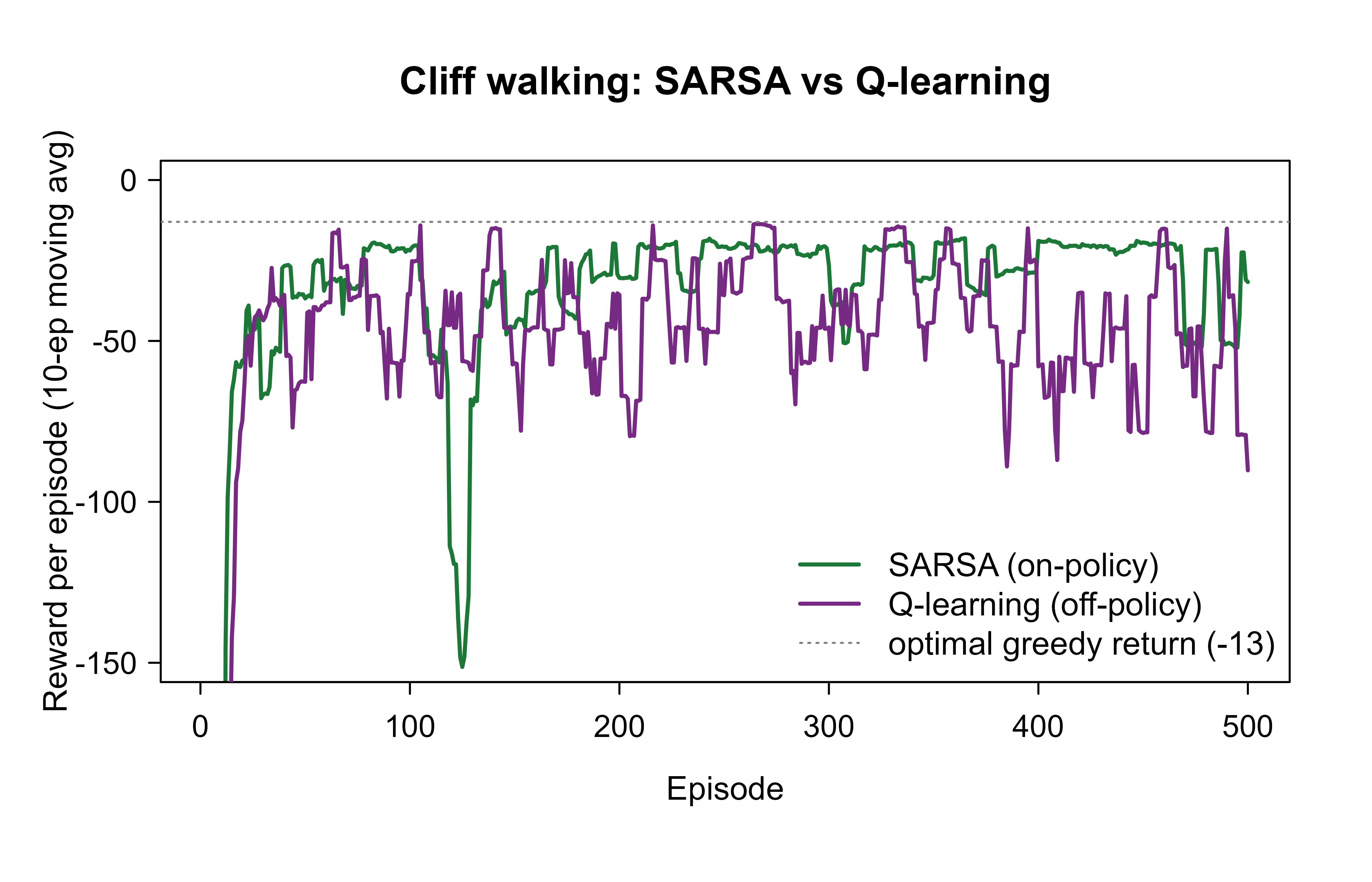
Figure 66.1 shows the reward collected per episode, smoothed with a trailing moving average so the trend is visible through the exploration noise. Both agents improve quickly. The instructive part is the steady state: Q-learning learns the optimal (shorter, riskier) path and so would score best if it never explored, but its \(\varepsilon\)-greedy exploration occasionally tips it off the cliff, dragging its online reward down. SARSA learns a safer path that keeps it away from the edge, so its online performance during learning is actually higher.
Show code
moving_avg<-function(x, k=10L){out<-rep(NA_real_, length(x))for(iinseq_along(x)){lo<-max(1L, i-k+1L)out[i]<-mean(x[lo:i])}out}sm_s<-moving_avg(sarsa$ep_reward)sm_q<-moving_avg(qlearn$ep_reward)plot(sm_s, type ="l", lwd =2, col ="#1b7837", ylim =c(-150, 0), xlab ="Episode", ylab ="Reward per episode (10-ep moving avg)", main ="Cliff walking: SARSA vs Q-learning")lines(sm_q, lwd =2, col ="#762a83")abline(h =-13, lty =3, col ="grey50")# optimal greedy path returnlegend("bottomright", legend =c("SARSA (on-policy)", "Q-learning (off-policy)","optimal greedy return (-13)"), col =c("#1b7837", "#762a83", "grey50"), lwd =c(2, 2, 1), lty =c(1, 1, 3), bty ="n")
Figure 66.1: Reward per episode (trailing 10-episode moving average) for SARSA and Q-learning on cliff walking. SARSA earns more online because it learns a safe path that tolerates its own exploration, while Q-learning’s optimal-but-risky path costs it occasional falls off the cliff.
66.5.2 The learned policies
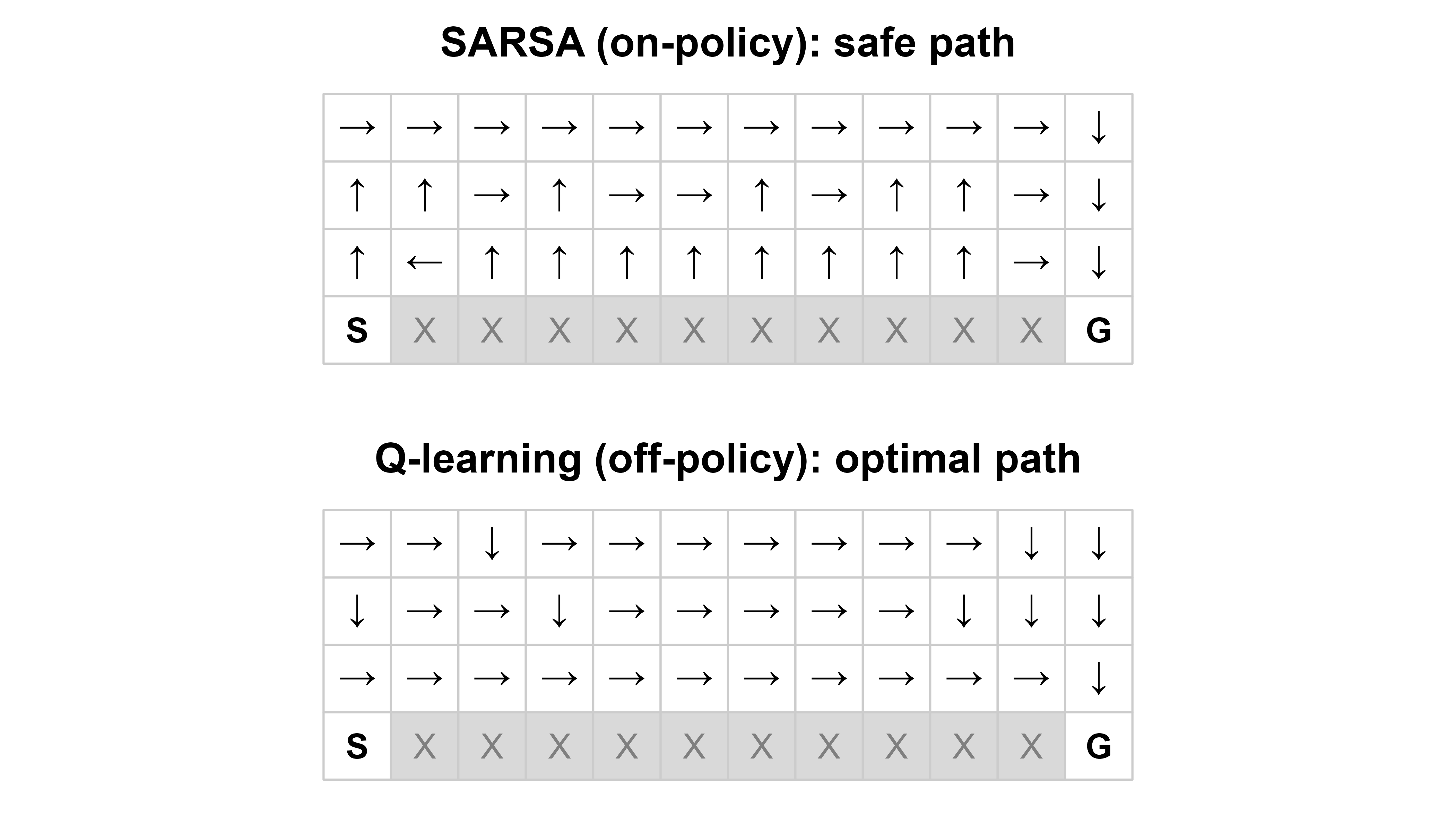
To see why the curves differ, we extract the greedy policy from each \(Q\) table and draw the grid. Figure 66.2 overlays both. Each arrow is the greedy action in that cell. Q-learning steers along the row directly above the cliff (the optimal path); SARSA climbs one extra row first, buying a safety margin against an unlucky random step.
Show code
arrow_for<-function(a)c("↑", "→", "↓", "←")[a]# up,right,down,leftdraw_policy<-function(Q, title){plot(NA, xlim =c(0.5, n_cols+0.5), ylim =c(0.5, n_rows+0.5), xlab ="", ylab ="", axes =FALSE, main =title, asp =1)for(sinseq_len(n_states)){row<-(s-1L)%/%n_cols+1Lcol<-(s-1L)%%n_cols+1Lrect(col-0.5, row-0.5, col+0.5, row+0.5, border ="grey80", col =if(s%in%cliff_states)"grey85"else"white")if(s%in%cliff_states){text(col, row, "X", col ="grey50")}elseif(s==start_state){text(col, row, "S", font =2)}elseif(s==goal_state){text(col, row, "G", font =2)}else{text(col, row, arrow_for(which.max(Q[s, ])), cex =1.1)}}}par(mfrow =c(2, 1), mar =c(1, 1, 2, 1))draw_policy(sarsa$Q, "SARSA (on-policy): safe path")draw_policy(qlearn$Q, "Q-learning (off-policy): optimal path")par(mfrow =c(1, 1))
Figure 66.2: Greedy policies recovered from the learned action-values. Left: SARSA takes the safe route, stepping up and away from the cliff edge. Right: Q-learning takes the optimal route hugging the cliff. ‘S’ marks start, ‘G’ goal, and shaded cells are the cliff.
66.5.3 Numerical comparison
Table 66.1 summarizes the contrast quantitatively, reporting the average online reward over the final 100 training episodes (when exploration is still on) for each method. The pattern is the classic result from Sutton and Barto (2018): SARSA’s online reward is higher even though Q-learning has learned the genuinely optimal policy.
Show code
final_window<-function(x, k=100L)mean(tail(x, k))comp<-data.frame( Property =c("Policy learned about", "Target uses","Path on this task", "Mean reward, last 100 ep","Behaviour when exploration off"), SARSA =c("the policy it follows (on-policy)","Q(S', A') with A' ~ eps-greedy","safe (one row above cliff)",sprintf("%.1f", final_window(sarsa$ep_reward)),"safe path"), `Q-learning` =c("the greedy/optimal policy (off-policy)","max_a Q(S', a)","optimal (along cliff edge)",sprintf("%.1f", final_window(qlearn$ep_reward)),"optimal path"), check.names =FALSE)knitr::kable(comp, caption ="SARSA versus Q-learning on cliff walking. SARSA collects more reward during learning because its on-policy target accounts for exploratory missteps; Q-learning's off-policy target learns the optimal path but pays for occasional exploratory falls.", booktabs =TRUE)
Table 66.1: SARSA versus Q-learning on cliff walking. SARSA collects more reward during learning because its on-policy target accounts for exploratory missteps; Q-learning’s off-policy target learns the optimal path but pays for occasional exploratory falls.
Property
SARSA
Q-learning
Policy learned about
the policy it follows (on-policy)
the greedy/optimal policy (off-policy)
Target uses
Q(S’, A’) with A’ ~ eps-greedy
max_a Q(S’, a)
Path on this task
safe (one row above cliff)
optimal (along cliff edge)
Mean reward, last 100 ep
-27.8
-52.8
Behaviour when exploration off
safe path
optimal path
66.6 Practical guidance and pitfalls
The demo is small, but the choices it exposes recur at every scale. A few practical points are worth carrying forward.
Choose on-policy or off-policy by what you need. Use SARSA (or its expected-value cousin, Expected SARSA) when the cost of exploratory mistakes during deployment is real, for instance a physical robot that should not learn a policy assuming it never slips. Use Q-learning when you can explore freely (in simulation, say) and want the optimal policy regardless of how you gathered the data. Off-policy learning is also what lets you learn from logged or historical experience, which on-policy methods cannot reuse cleanly; learning purely from a fixed dataset is the subject of the offline reinforcement learning chapter (Chapter 69).
When to use this
Reach for TD control over Monte Carlo whenever episodes are long, never-ending, or you need to learn online. Prefer Monte Carlo when the environment is not really Markov in your state representation, since MC does not rely on the bootstrapping assumption that the next state’s value is a valid summary of the future.
Set the step size and exploration with care. A constant \(\alpha\) (we used \(0.5\)) never fully converges but adapts to change, which is usually what you want; if you need convergence to a fixed answer, decay \(\alpha\) over time. Exploration \(\varepsilon\) governs the safe-versus-optimal gap directly: as \(\varepsilon \to 0\), SARSA’s safe path converges to the same optimal path Q-learning already prefers, because there are no more random missteps to guard against. Many implementations anneal \(\varepsilon\) from high to low so the agent explores early and exploits late.
Watch for maximization bias. The \(\max\) in Q-learning’s target systematically overestimates action-values when those values are noisy, because the maximum of noisy estimates is biased upward. Double Q-learning fixes this by keeping two value tables and using one to select the action and the other to evaluate it. Be aware too that the convergence guarantees in this chapter are for the tabular case, one entry per state-action pair. The moment you replace the table with a function approximator and combine it with bootstrapping and off-policy updates (the “deadly triad”), stability is no longer free; this is the territory of the deep reinforcement learning chapter (Chapter 71).
Warning
Do not read the cliff-walking result as “SARSA is better than Q-learning.” Q-learning learned the better policy; SARSA earned more during training because it was being judged while still exploring. With exploration turned off at deployment, Q-learning’s policy wins. The lesson is to match the algorithm to whether mistakes made while learning actually count.
Finally, mind credit assignment over long horizons. One-step TD propagates a reward backward only one state per episode, so a sparse goal reward can take many episodes to reach the start. This is exactly the gap eligibility traces (TD(\(\lambda\))) close, and in sparse-reward problems a moderate \(\lambda\) (around \(0.8\) to \(0.9\)) often learns dramatically faster than TD(0) at little extra cost.
66.7 Further reading
The definitive treatment is Sutton and Barto, Reinforcement Learning: An Introduction (2nd edition, 2018), whose Chapters 5, 6, and 12 cover Monte Carlo methods, temporal-difference learning, and eligibility traces respectively; the cliff-walking example used here is their Example 6.6. The original TD(0) analysis is Sutton (1988), “Learning to Predict by the Methods of Temporal Differences.” Q-learning and its convergence proof are due to Watkins (1989) and Watkins and Dayan (1992). For a graduate-level, more mathematical perspective, see Bertsekas and Tsitsiklis, Neuro-Dynamic Programming (1996), and Szepesvari, Algorithms for Reinforcement Learning (2010). For maximization bias and its remedy, see van Hasselt (2010) on Double Q-learning.
The flip side is that Monte Carlo is unbiased. Each sampled return is an honest draw from the true return distribution, so the only error is variance, which averaging drives down. TD trades some of this away, accepting bias from bootstrapping in exchange for much lower variance.↩︎
Source Code
# Monte Carlo and Temporal-Difference Learning {#sec-td-learning}```{r}#| include: falsesource("_common.R")```Suppose you are dropped into an unfamiliar building and told there is an exit somewhere, with a small reward waiting outside. Nobody hands you a floor plan. You can only walk around, occasionally bump into a wall, and eventually stumble out the door. Do this many times and something useful happens: you start to sense which corridors lead somewhere good and which dead-end, long before you can articulate the building's layout. You learn to act well without ever writing down a map.That is the situation this chapter studies. In the language of Markov decision processes, the "map" is the transition model (where each action takes you) together with the reward function (what each move pays). When you know both, you can solve for the optimal behavior by dynamic programming: value iteration and policy iteration sweep through the known dynamics and compute the best policy directly (see the foundations of reinforcement learning chapter, @sec-rl-foundations). But in most real problems the dynamics are unknown. A robot does not know in advance how its motors interact with a slippery floor; a recommendation agent does not know how a user will react to a new layout. The agent has to learn purely from experience, one transition at a time. This is the *model-free* setting, and it is where Monte Carlo and temporal-difference (TD) methods live.The two ideas in the title sit at opposite ends of a spectrum. Monte Carlo methods wait until an episode finishes and then learn from the total reward actually collected: honest but patient. Temporal-difference methods update after every single step, using their own current guess of the future as a stand-in for the rest of the episode: a guess that bootstraps off another guess. That sounds circular, and the surprising fact, made precise below, is that it works, often far better than waiting. By the end of the chapter you will understand the TD update and the TD error, see why SARSA and Q-learning differ by a single symbol yet behave differently near danger, and have a runnable base-R agent that learns to walk along a cliff without falling off.::: {.callout-note}This chapter assumes you have met the Markov decision process (MDP) and the Bellman equations, for instance through value iteration on a known model. Here the model is unknown. Everything is learned from sampled experience: tuples of state, action, reward, and next state.:::## Notation and the prediction problem {#td-notation}We work with a finite MDP. At each time step $t$ the agent is in a state $S_t \in \mathcal{S}$, takes an action $A_t \in \mathcal{A}$, receives a scalar reward $R_{t+1} \in \mathbb{R}$, and moves to a new state $S_{t+1}$. A *policy* $\pi(a \mid s)$ gives the probability of choosing action $a$ in state $s$. The agent's goal is to maximize the expected *return*, the discounted sum of future rewards$$G_t \;=\; R_{t+1} + \gamma R_{t+2} + \gamma^2 R_{t+3} + \cdots \;=\; \sum_{k=0}^{\infty} \gamma^k R_{t+k+1},$$where the *discount factor* $\gamma \in [0,1]$ trades off immediate against later reward. A value of $\gamma$ near $0$ makes the agent myopic; near $1$ it cares about the distant future.Two value functions summarize how good things are under a policy $\pi$:$$v_\pi(s) = \mathbb{E}_\pi[\,G_t \mid S_t = s\,], \qquadq_\pi(s,a) = \mathbb{E}_\pi[\,G_t \mid S_t = s,\, A_t = a\,].$$The *state-value* $v_\pi(s)$ is the expected return from $s$ onward; the *action-value* $q_\pi(s,a)$ is the expected return after committing to action $a$ in $s$ and following $\pi$ afterward. Because the model is unknown, action-values are the more useful object: if you know $q$, you can act greedily by picking $\arg\max_a q(s,a)$ without ever consulting a transition model. Learning $v_\pi$ or $q_\pi$ for a fixed $\pi$ is the *prediction* problem; improving $\pi$ toward the optimal policy $\pi_*$ is the *control* problem.::: {.callout-important title="Key idea"}When the dynamics are unknown, action-values $q(s,a)$ are worth more than state-values $v(s)$, because choosing the best action from $q$ needs no model, whereas choosing from $v$ requires knowing where each action would take you.:::### The Bellman operator and its fixed point {#td-bellman-operator}All the convergence results in this chapter rest on a single structural fact: the value function is the unique fixed point of a contraction mapping. Making this precise pays off later, because every algorithm here is a sampled, stochastic version of applying that mapping.Conditioning the return identity $G_t = R_{t+1} + \gamma G_{t+1}$ on $S_t = s$ and taking expectations under $\pi$ gives the Bellman expectation equation$$v_\pi(s) \;=\; \sum_{a} \pi(a \mid s) \sum_{s', r} p(s', r \mid s, a)\,\bigl[\, r + \gamma\, v_\pi(s') \,\bigr],$$ {#eq-td-learning-bellman-exp}where $p(s', r \mid s, a)$ is the (unknown) joint transition-reward kernel. Collect the values into a vector $v \in \mathbb{R}^{|\mathcal{S}|}$ and define the *Bellman expectation operator* $T^\pi : \mathbb{R}^{|\mathcal{S}|} \to \mathbb{R}^{|\mathcal{S}|}$ componentwise by$$(T^\pi v)(s) \;=\; \mathbb{E}_\pi\!\bigl[\, R_{t+1} + \gamma\, v(S_{t+1}) \mid S_t = s \,\bigr] \;=\; r_\pi(s) + \gamma \sum_{s'} P_\pi(s, s')\, v(s'),$$ {#eq-td-learning-bellman-op}with $r_\pi(s) = \mathbb{E}_\pi[R_{t+1} \mid S_t = s]$ the expected one-step reward and $P_\pi$ the state-to-state transition matrix induced by $\pi$. Equation @eq-td-learning-bellman-exp says exactly that $v_\pi$ satisfies $T^\pi v_\pi = v_\pi$, i.e. $v_\pi$ is a fixed point of $T^\pi$.This fixed point is unique and globally attracting because $T^\pi$ is a $\gamma$-contraction in the sup-norm. For any two value vectors $u, w$,$$\|T^\pi u - T^\pi w\|_\infty= \gamma \,\bigl\| P_\pi (u - w) \bigr\|_\infty\le \gamma \,\|P_\pi\|_\infty \,\|u - w\|_\infty= \gamma \,\|u - w\|_\infty,$$ {#eq-td-learning-contraction}where the last equality uses $\|P_\pi\|_\infty = 1$ because each row of $P_\pi$ is a probability distribution and therefore sums to one with nonnegative entries. For $\gamma < 1$ this is a strict contraction, so by the Banach fixed-point theorem $T^\pi$ has a unique fixed point and the iteration $v_{k+1} = T^\pi v_k$ converges geometrically, $\|v_k - v_\pi\|_\infty \le \gamma^k \|v_0 - v_\pi\|_\infty$, from any start $v_0$. The action-value analogue $q_\pi = T^\pi q_\pi$ and the optimal-value operator $(T^* v)(s) = \max_a \mathbb{E}[R_{t+1} + \gamma v(S_{t+1}) \mid s, a]$ are contractions by the same argument (the $\max$ is nonexpansive), giving the optimal value functions $v_*, q_*$ as their fixed points. TD(0) replaces the expectation in $T^\pi$ with a single sample, and Q-learning replaces the expectation in $T^*$ with a single sample; that is the entire conceptual content of both algorithms.::: {.callout-note}The contraction is in the *weighted* or sup norm, not in Euclidean norm. This distinction is harmless in the tabular case but becomes the crux of stability once linear function approximation enters: $T^\pi$ is a contraction in the $\mu_\pi$-weighted norm (with $\mu_\pi$ the stationary distribution) for on-policy sampling, which is why on-policy TD with linear features converges while off-policy TD need not.:::## Monte Carlo: learn from complete returns {#td-monte-carlo}The most direct way to estimate $v_\pi(s)$ is to take its definition literally. Run the policy, record the return that actually followed each visit to $s$, and average those returns. By the law of large numbers the average converges to the expectation. This is the Monte Carlo (MC) idea, and it requires only the ability to sample episodes, not any knowledge of transition probabilities.Concretely, suppose state $s$ was visited and the episode that followed yielded return $G$. The *every-visit* MC estimate maintains a running average$$V(s) \;\leftarrow\; V(s) + \alpha \,\bigl[\, G - V(s) \,\bigr],$$where $\alpha$ is a step size (using $\alpha = 1/N(s)$, with $N(s)$ the visit count, recovers the exact sample mean). The quantity $G - V(s)$ is the error between the realized return and the current estimate, and we nudge $V(s)$ a fraction of the way toward $G$.The defining feature, and the catch, is that $G$ is only known once the episode terminates. Monte Carlo cannot learn from an unfinished episode, and it cannot be used at all in a setting that never ends. It is also high variance: a single episode's return depends on every random action and transition along the way, so estimates wobble.^[The flip side is that Monte Carlo is unbiased. Each sampled return is an honest draw from the true return distribution, so the only error is variance, which averaging drives down. TD trades some of this away, accepting bias from bootstrapping in exchange for much lower variance.]::: {.callout-tip title="Intuition"}Monte Carlo is like grading a chess move only by who won the game. Correct on average, but you must play to the end, and a single blunder elsewhere can wrongly tar a good move.:::## Temporal-difference learning: bootstrap from the next step {#td-zero}Temporal-difference learning keeps the averaging idea but refuses to wait. The insight is that the return obeys a recursive relationship, the Bellman equation: $G_t = R_{t+1} + \gamma G_{t+1}$. We cannot observe $G_{t+1}$, but we already maintain an estimate of its expectation, namely $V(S_{t+1})$. So we substitute the estimate for the unknown and update immediately after one step. This is the TD(0) update:$$V(S_t) \;\leftarrow\; V(S_t) + \alpha \,\underbrace{\bigl[\, R_{t+1} + \gamma V(S_{t+1}) - V(S_t) \,\bigr]}_{\displaystyle \delta_t},$$The bracketed quantity $\delta_t$ is the *TD error*. It compares two estimates of the same thing: the one-step *target* $R_{t+1} + \gamma V(S_{t+1})$, which mixes a real observed reward with a bootstrapped guess of the rest, against the current estimate $V(S_t)$. If the target exceeds the estimate, $S_t$ was better than we thought and we raise its value; if lower, we lower it.::: {.callout-important title="Key idea"}The TD error $\delta_t = R_{t+1} + \gamma V(S_{t+1}) - V(S_t)$ is the engine of reinforcement learning. It measures surprise: the gap between what you expected and what one real step plus your own forecast now tell you. Every algorithm in this chapter is, at bottom, a rule for reducing TD error.:::Replacing the full return $G_t$ with the bootstrapped target $R_{t+1} + \gamma V(S_{t+1})$ has three consequences. First, you can learn online, after every step, even in problems that never terminate. Second, the target depends on only one random reward and transition rather than the whole future, so its variance is far lower than Monte Carlo's. Third, the target is biased while $V$ is still wrong, because it leans on a guess. In practice the variance reduction usually dominates, and TD methods tend to learn faster on Markov problems. Both MC and TD(0) converge to $v_\pi$ under standard step-size conditions, but they take different routes there.::: {.callout-note}The Robbins-Monro conditions on the step size, $\sum_t \alpha_t = \infty$ and $\sum_t \alpha_t^2 < \infty$, guarantee convergence for the prediction problem. A constant $\alpha$ violates the second condition and so does not fully converge; instead it tracks a moving target, which is exactly what you want in a nonstationary environment.:::### TD(0) as stochastic approximation {#td-stochastic-approximation}The TD(0) update is not an ad hoc heuristic; it is the Robbins-Monro stochastic-approximation scheme applied to the Bellman fixed-point equation, and recognizing this both explains why it converges and tells us what it converges to.Stochastic approximation solves a root-finding problem $\bar g(v) = 0$ when we cannot evaluate $\bar g$ directly but can draw noisy samples $g_t$ with $\mathbb{E}[g_t \mid v] = \bar g(v)$. The iteration $v \leftarrow v + \alpha_t\, g_t$ converges to a root under the Robbins-Monro step-size conditions. Take the root-finding target to be the Bellman residual at state $s$,$$\bar g(V)(s) \;=\; (T^\pi V)(s) - V(s) \;=\; \mathbb{E}_\pi\!\bigl[\, R_{t+1} + \gamma V(S_{t+1}) - V(S_t) \mid S_t = s \,\bigr],$$ {#eq-td-learning-td-mean}whose unique root is $V = v_\pi$ by @eq-td-learning-bellman-op. The TD error $\delta_t = R_{t+1} + \gamma V(S_{t+1}) - V(S_t)$ is exactly an unbiased one-sample estimate of this residual, because conditioning on $S_t = s$ and the current $V$,$$\mathbb{E}_\pi[\delta_t \mid S_t = s] \;=\; (T^\pi V)(s) - V(s) \;=\; \bar g(V)(s).$$ {#eq-td-learning-td-unbiased}So $V(S_t) \leftarrow V(S_t) + \alpha\, \delta_t$ is precisely Robbins-Monro on @eq-td-learning-td-mean. Under the standard step-size conditions, with every state visited infinitely often and bounded rewards, the iterates converge with probability one to the fixed point $v_\pi$ (Sutton 1988; Jaakkola, Jordan, and Singh 1994; Tsitsiklis 1994). The bias seen in finite samples comes entirely from the fact that the noisy target $R_{t+1} + \gamma V(S_{t+1})$ uses the current $V$ rather than the true $v_\pi$: $\mathbb{E}[\delta_t]$ is unbiased *for the residual at the current $V$*, not for the residual at $v_\pi$, which is what bootstrapping costs.::: {.callout-note}The same lens identifies Q-learning as Robbins-Monro on the *optimal* Bellman residual $\bar g(Q)(s,a) = (T^* Q)(s,a) - Q(s,a)$, whose root is $q_*$. Because $T^*$ involves a $\max$ and not the behavior policy, the sampled residual remains unbiased for $T^* Q - Q$ regardless of how actions are chosen, which is the formal reason Q-learning is off-policy. SARSA instead samples $T^\pi Q - Q$ for the *current* $\pi$, so it tracks a moving target as $\pi$ improves.:::### What TD and Monte Carlo converge to: the batch fixed points {#td-batch-fixed-point}TD and MC both converge to $v_\pi$ asymptotically, but with finite data they answer two genuinely different questions, and the difference is sharpest in the *batch* setting. Suppose we have a fixed set of episodes and replay it repeatedly, applying each update with a tiny step size until the estimates stop moving (the batch limit). What does each method settle on?Batch Monte Carlo minimizes the in-sample mean squared error to the observed returns. For each state it returns the average of the returns that actually followed visits to that state:$$V_{\mathrm{MC}}(s) \;=\; \arg\min_{V} \sum_{\text{visits to } s} \bigl(\, G - V(s) \,\bigr)^2 \;=\; \frac{1}{N(s)} \sum_{\text{visits to } s} G.$$ {#eq-td-learning-batch-mc}Batch TD(0) instead converges to the *certainty-equivalence* estimate: it builds the maximum-likelihood MDP from the data (empirical transition frequencies $\hat p$ and empirical mean rewards $\hat r$) and reports the exact value function of that estimated model,$$V_{\mathrm{TD}}(s) \;=\; \hat r(s) + \gamma \sum_{s'} \hat P(s, s')\, V_{\mathrm{TD}}(s'),$$ {#eq-td-learning-batch-td}the solution of the empirical Bellman equation. This is why batch TD can be *more accurate* than batch MC on a Markov problem with limited data: MC ignores the Markov structure and treats each state's returns in isolation, whereas TD exploits the structure by stitching together transitions, effectively pooling information across episodes. The classic illustration is Sutton and Barto's "A/B" example (2018, Example 6.4): given episodes in which state B is sometimes followed by reward and A is always followed by B, MC assigns $V(A)$ the single observed return through A, while TD assigns $V(A) = \gamma V(B)$, propagating B's better-estimated value backward. On a truly Markov problem the certainty-equivalence estimate @eq-td-learning-batch-td is the statistically efficient one; when the Markov assumption fails, MC's model-free average @eq-td-learning-batch-mc can be safer, which is the principled reason to prefer MC in non-Markov state representations.::: {.callout-tip title="Intuition"}MC asks "what return did I actually see from here?" TD asks "what return does my best model of the world predict from here?" When the world really is Markov, the model-based answer wins because it borrows strength across all transitions; when your states secretly hide relevant history, the model is wrong and the raw average is the honest choice.:::### TD(lambda) and eligibility traces, conceptually {#td-lambda}TD(0) looks one step ahead; Monte Carlo looks all the way to the end. There is a whole family in between. The $n$-step return $G_t^{(n)} = R_{t+1} + \gamma R_{t+2} + \cdots + \gamma^{n-1} R_{t+n} + \gamma^n V(S_{t+n})$ uses $n$ real rewards before bootstrapping. TD(0) is $n=1$; Monte Carlo is $n = \infty$.TD($\lambda$) blends all of these at once. It forms a geometrically weighted average of every $n$-step return, controlled by a single parameter $\lambda \in [0,1]$:$$G_t^\lambda \;=\; (1-\lambda) \sum_{n=1}^{\infty} \lambda^{\,n-1} G_t^{(n)}.$$At $\lambda = 0$ only the one-step return survives and we recover TD(0); at $\lambda = 1$ the average collapses to the full return and we recover Monte Carlo. The practical implementation does not literally compute that infinite sum. Instead it keeps an *eligibility trace* $e(s)$ for each state: a short-term memory that spikes when a state is visited and then fades by a factor $\gamma\lambda$ each step. When a TD error occurs, every state is updated in proportion to its current trace, so credit flows backward to recently visited states. This lets a single surprising reward at the goal propagate to the steps that led there, rather than seeping back one state per episode.::: {.callout-tip title="Intuition"}Eligibility traces answer "who deserves credit for this surprise?" A state visited one step ago is highly eligible; a state visited twenty steps ago, only faintly. The trace is the fading footprint the agent leaves behind, and the TD error is splashed back along it.:::## Control: SARSA and Q-learning {#td-control}Prediction estimates the value of a fixed policy. Control improves the policy. The standard recipe is *generalized policy iteration*: alternate between estimating action-values $Q(s,a)$ and acting greedily with respect to them. To keep exploring, the agent does not act purely greedily but follows an *$\varepsilon$-greedy* policy: with probability $1-\varepsilon$ take $\arg\max_a Q(s,a)$, and with probability $\varepsilon$ take a uniformly random action. The two famous control algorithms differ only in how they form the TD target.SARSA is *on-policy*. Its name lists the tuple it uses: $(S_t, A_t, R_{t+1}, S_{t+1}, A_{t+1})$. It actually chooses the next action $A_{t+1}$ from its current ($\varepsilon$-greedy) policy and uses that action's value in the target:$$Q(S_t, A_t) \;\leftarrow\; Q(S_t, A_t) + \alpha \,\bigl[\, R_{t+1} + \gamma\, Q(S_{t+1}, A_{t+1}) - Q(S_t, A_t) \,\bigr].$$Because $A_{t+1}$ is drawn from the same policy the agent follows, SARSA evaluates and improves the policy it is genuinely using, exploration included.Q-learning is *off-policy*. It targets the value of the *best* next action regardless of what it actually does next:$$Q(S_t, A_t) \;\leftarrow\; Q(S_t, A_t) + \alpha \,\bigl[\, R_{t+1} + \gamma \max_{a} Q(S_{t+1}, a) - Q(S_t, A_t) \,\bigr].$$The $\max$ over actions makes the target track the greedy (optimal) policy even while the agent behaves $\varepsilon$-greedily. So Q-learning learns about a policy it does not follow: it explores with randomness but learns the value of acting greedily.::: {.callout-important title="Key idea"}SARSA and Q-learning differ by one symbol in the target. SARSA uses $Q(S_{t+1}, A_{t+1})$, the value of the action it will take. Q-learning uses $\max_a Q(S_{t+1}, a)$, the value of the best action it could take. On-policy versus off-policy hinges entirely on that choice.:::This difference is not cosmetic. SARSA's target accounts for the fact that the agent will sometimes explore and land somewhere bad, so it learns a policy that is cautious in the presence of its own randomness. Q-learning assumes greedy behavior in the target and so learns the optimal policy's values, even though its random exploration occasionally pushes it into trouble. The cliff-walking demo below makes the consequence vivid: SARSA prefers a safe detour, Q-learning hugs the cliff edge.### Expected SARSA: removing the action-sampling variance {#td-expected-sarsa}SARSA's target uses a single sampled next action $A_{t+1}$, which injects variance from the policy's randomness on top of the environment's. Expected SARSA removes that source by replacing the sampled action with its expectation under the policy, computing the target in closed form,$$Q(S_t, A_t) \;\leftarrow\; Q(S_t, A_t) + \alpha \,\Bigl[\, R_{t+1} + \gamma \sum_{a} \pi(a \mid S_{t+1})\, Q(S_{t+1}, a) - Q(S_t, A_t) \,\Bigr].$$ {#eq-td-learning-expected-sarsa}The target is now the exact conditional expectation $\mathbb{E}_{A_{t+1} \sim \pi}[Q(S_{t+1}, A_{t+1}) \mid S_{t+1}]$, so by the law of total variance Expected SARSA has the same expected update as SARSA but strictly lower variance whenever $Q(S_{t+1}, \cdot)$ is not constant in the action. This lets it use a larger step size and often dominates ordinary SARSA empirically. It also unifies the chapter's algorithms: under a greedy target policy, $\pi(a \mid s) = \mathbb{1}\{a = \arg\max_{a'} Q(s, a')\}$, the sum in @eq-td-learning-expected-sarsa collapses to $\max_a Q(S_{t+1}, a)$ and Expected SARSA *is* Q-learning. Under the agent's own $\varepsilon$-greedy policy it is the variance-reduced version of SARSA. Expected SARSA can be run on-policy or, by choosing a target policy different from the behavior policy, off-policy, making it a strict generalization of both endpoints.### Convergence, bias, variance, and complexity {#td-control-theory}The tabular control algorithms inherit the stochastic-approximation guarantees of the prediction case, with one extra requirement for the optimality argument. Q-learning converges with probability one to $q_*$ provided every state-action pair is visited infinitely often and the step sizes satisfy the Robbins-Monro conditions (Watkins and Dayan 1992; Tsitsiklis 1994); notably the behavior policy may be anything that keeps exploring, since the $\max$ target does not depend on it. SARSA converges to $q_*$ only if the policy is additionally *greedy in the limit with infinite exploration* (GLIE), for example by annealing $\varepsilon_t \to 0$ slowly enough; otherwise it converges to the action-values of the limiting $\varepsilon$-greedy policy, which is precisely why it learns the safe path while exploration persists.The error of these estimators decomposes along the usual axes. The variance of a single update scales with $\alpha$ and with the conditional variance of the target; under a decaying step size $\alpha_t \asymp 1/t$ the mean squared error of stochastic approximation decays at the optimal $O(1/t)$ rate, while a well-tuned constant $\alpha$ reaches an $O(\alpha)$ error floor much faster, which is the bias-variance trade governing step-size choice in practice. The bias is the bootstrapping bias: the target leans on the current, still-wrong $Q$, so $\mathbb{E}[\delta_t]$ measures the residual at the current estimate rather than at $q_*$. Across the $n$-step spectrum, larger $n$ (toward Monte Carlo) reduces bias but raises variance, while smaller $n$ (toward TD(0)) does the reverse; TD($\lambda$) interpolates with a single knob. Per update the cost is $O(1)$ for tabular SARSA and Q-learning and $O(|\mathcal{A}|)$ for Expected SARSA, with memory $O(|\mathcal{S}|\,|\mathcal{A}|)$ for the table, so the methods are cheap and the binding constraint is sample complexity, the number of transitions needed, not computation per step.#### Maximization bias, quantified {#td-max-bias}Q-learning's $\max$ target overestimates because the maximum of unbiased noisy estimates is biased upward. Suppose the true action-values at a state are all equal, $q(s,a) = \mu$ for every $a$, but we hold independent unbiased estimates $\hat Q(s,a)$ with variance $\sigma^2$. The Q-learning target uses $\max_a \hat Q(s,a)$, and by Jensen's inequality applied to the convex $\max$,$$\mathbb{E}\Bigl[\, \max_a \hat Q(s,a) \,\Bigr] \;\ge\; \max_a \mathbb{E}\bigl[\hat Q(s,a)\bigr] \;=\; \mu,$$ {#eq-td-learning-max-bias}with a strictly positive gap that grows with $\sigma^2$ and with the number of actions $|\mathcal{A}|$ (for $|\mathcal{A}|$ independent Gaussians the gap scales roughly like $\sigma \sqrt{2 \log |\mathcal{A}|}$). This positive bias propagates backward through bootstrapping and can substantially inflate value estimates in noisy or stochastic environments. Double Q-learning removes it by decoupling selection from evaluation: it keeps two tables $Q^A, Q^B$, uses one to pick the maximizing action and the *other* to score it, $Q^B(s', \arg\max_a Q^A(s', a))$, so the evaluated value is unbiased for the selected action. The argument runs both ways, eliminating the systematic overestimate at the cost of doubled memory and a slight underestimate in some settings.The following short simulation confirms @eq-td-learning-max-bias and the double-estimator fix. With true value $\mu = 0$ for every action, the single-max estimator is biased upward while the decoupled estimator is essentially unbiased.```{r td-learning-maxbias}set.seed(1301)mu <-0; sigma <-1; n_actions_sim <-10L; n_rep <-50000Lsingle <-numeric(n_rep); double_est <-numeric(n_rep)for (i inseq_len(n_rep)) { qa <-rnorm(n_actions_sim, mu, sigma) # estimator A qb <-rnorm(n_actions_sim, mu, sigma) # estimator B (independent) single[i] <-max(qa) # single-max: biased up double_est[i] <- qb[which.max(qa)] # select with A, evaluate with B}c(single_max_bias =mean(single), double_est_bias =mean(double_est),predicted_gap = sigma *sqrt(2*log(n_actions_sim)))```## A runnable demo: cliff walking {#td-demo}We implement both algorithms in base R on the cliff-walking gridworld of Sutton and Barto (2018, Example 6.6). The grid is 4 rows by 12 columns. The start is the bottom-left cell and the goal is the bottom-right. The entire bottom row between them is a cliff. Every step costs $-1$. Stepping into the cliff costs $-100$ and teleports the agent back to the start. Actions are the four moves up, down, left, right; moving into an outer wall leaves the agent in place.The optimal path (in terms of total reward) runs straight along the row just above the cliff. But that path is risky for an exploring agent: a single random step downward falls off. We will see the two algorithms resolve this tension differently.```{r td-learning-setup}set.seed(1301)# Cliff-walking environment ------------------------------------------------n_rows <-4Ln_cols <-12Ln_states <- n_rows * n_colsn_actions <-4L # 1=up, 2=right, 3=down, 4=left# Map (row, col) with row 1 at the BOTTOM to a state index 1..48.rc_to_state <-function(row, col) (row -1L) * n_cols + colstart_state <-rc_to_state(1L, 1L)goal_state <-rc_to_state(1L, n_cols)# Cliff cells: bottom row, columns 2..11.cliff_states <-rc_to_state(1L, 2L:(n_cols -1L))# Given a state and action, return list(next_state, reward, done).step_env <-function(s, a) { row <- (s -1L) %/% n_cols +1L col <- (s -1L) %% n_cols +1Lif (a ==1L) row <-min(row +1L, n_rows) # upif (a ==2L) col <-min(col +1L, n_cols) # rightif (a ==3L) row <-max(row -1L, 1L) # downif (a ==4L) col <-max(col -1L, 1L) # left s2 <-rc_to_state(row, col)if (s2 %in% cliff_states) {return(list(next_state = start_state, reward =-100, done =FALSE)) }if (s2 == goal_state) {return(list(next_state = s2, reward =-1, done =TRUE)) }list(next_state = s2, reward =-1, done =FALSE)}# epsilon-greedy action selection from a Q-row.eps_greedy <-function(qrow, epsilon) {if (runif(1) < epsilon) {sample.int(n_actions, 1L) } else {which.max(qrow) # ties: first max, deterministic }}```The two learners share almost all of their code. We write one function with a flag selecting the target.```{r td-learning-agents}run_agent <-function(method =c("sarsa", "qlearning"),n_episodes =500L,alpha =0.5, gamma =1.0, epsilon =0.1,max_steps =1000L) { method <-match.arg(method) Q <-matrix(0, nrow = n_states, ncol = n_actions) ep_reward <-numeric(n_episodes)for (ep inseq_len(n_episodes)) { s <- start_state a <-eps_greedy(Q[s, ], epsilon) total <-0 done <-FALSE steps <-0Lwhile (!done && steps < max_steps) { steps <- steps +1L res <-step_env(s, a) s2 <- res$next_state; r <- res$reward; done <- res$done total <- total + rif (method =="sarsa") { a2 <-eps_greedy(Q[s2, ], epsilon) # on-policy next action target <- r + gamma * Q[s2, a2] * (!done) } else { a2 <-eps_greedy(Q[s2, ], epsilon) # behaviour is still eps-greedy target <- r + gamma *max(Q[s2, ]) * (!done) # off-policy: greedy target } Q[s, a] <- Q[s, a] + alpha * (target - Q[s, a]) s <- s2; a <- a2 } ep_reward[ep] <- total }list(Q = Q, ep_reward = ep_reward)}set.seed(1301)sarsa <-run_agent("sarsa")set.seed(1301)qlearn <-run_agent("qlearning")```### Learning curves {#td-demo-curve}@fig-td-learning-curve shows the reward collected per episode, smoothed with a trailing moving average so the trend is visible through the exploration noise. Both agents improve quickly. The instructive part is the steady state: Q-learning learns the optimal (shorter, riskier) path and so would score best if it never explored, but its $\varepsilon$-greedy exploration occasionally tips it off the cliff, dragging its online reward down. SARSA learns a safer path that keeps it away from the edge, so its online performance during learning is actually higher.```{r fig-td-learning-curve, fig.cap="Reward per episode (trailing 10-episode moving average) for SARSA and Q-learning on cliff walking. SARSA earns more online because it learns a safe path that tolerates its own exploration, while Q-learning's optimal-but-risky path costs it occasional falls off the cliff.", fig.width=7, fig.height=4.5}moving_avg <-function(x, k =10L) { out <-rep(NA_real_, length(x))for (i inseq_along(x)) { lo <-max(1L, i - k +1L) out[i] <-mean(x[lo:i]) } out}sm_s <-moving_avg(sarsa$ep_reward)sm_q <-moving_avg(qlearn$ep_reward)plot(sm_s, type ="l", lwd =2, col ="#1b7837",ylim =c(-150, 0), xlab ="Episode",ylab ="Reward per episode (10-ep moving avg)",main ="Cliff walking: SARSA vs Q-learning")lines(sm_q, lwd =2, col ="#762a83")abline(h =-13, lty =3, col ="grey50") # optimal greedy path returnlegend("bottomright",legend =c("SARSA (on-policy)", "Q-learning (off-policy)","optimal greedy return (-13)"),col =c("#1b7837", "#762a83", "grey50"),lwd =c(2, 2, 1), lty =c(1, 1, 3), bty ="n")```### The learned policies {#td-demo-policy}To see *why* the curves differ, we extract the greedy policy from each $Q$ table and draw the grid. @fig-td-learning-policies overlays both. Each arrow is the greedy action in that cell. Q-learning steers along the row directly above the cliff (the optimal path); SARSA climbs one extra row first, buying a safety margin against an unlucky random step.```{r fig-td-learning-policies, fig.cap="Greedy policies recovered from the learned action-values. Left: SARSA takes the safe route, stepping up and away from the cliff edge. Right: Q-learning takes the optimal route hugging the cliff. 'S' marks start, 'G' goal, and shaded cells are the cliff.", fig.width=7, fig.height=4}arrow_for <-function(a) c("↑", "→", "↓", "←")[a] # up,right,down,leftdraw_policy <-function(Q, title) {plot(NA, xlim =c(0.5, n_cols +0.5), ylim =c(0.5, n_rows +0.5),xlab ="", ylab ="", axes =FALSE, main = title, asp =1)for (s inseq_len(n_states)) { row <- (s -1L) %/% n_cols +1L col <- (s -1L) %% n_cols +1Lrect(col -0.5, row -0.5, col +0.5, row +0.5, border ="grey80",col =if (s %in% cliff_states) "grey85"else"white")if (s %in% cliff_states) {text(col, row, "X", col ="grey50") } elseif (s == start_state) {text(col, row, "S", font =2) } elseif (s == goal_state) {text(col, row, "G", font =2) } else {text(col, row, arrow_for(which.max(Q[s, ])), cex =1.1) } }}par(mfrow =c(2, 1), mar =c(1, 1, 2, 1))draw_policy(sarsa$Q, "SARSA (on-policy): safe path")draw_policy(qlearn$Q, "Q-learning (off-policy): optimal path")par(mfrow =c(1, 1))```### Numerical comparison {#td-demo-table}@tbl-td-learning-compare summarizes the contrast quantitatively, reporting the average online reward over the final 100 training episodes (when exploration is still on) for each method. The pattern is the classic result from Sutton and Barto (2018): SARSA's online reward is higher even though Q-learning has learned the genuinely optimal policy.```{r tbl-td-learning-compare}final_window <-function(x, k =100L) mean(tail(x, k))comp <-data.frame(Property =c("Policy learned about", "Target uses","Path on this task", "Mean reward, last 100 ep","Behaviour when exploration off"),SARSA =c("the policy it follows (on-policy)","Q(S', A') with A' ~ eps-greedy","safe (one row above cliff)",sprintf("%.1f", final_window(sarsa$ep_reward)),"safe path"),`Q-learning`=c("the greedy/optimal policy (off-policy)","max_a Q(S', a)","optimal (along cliff edge)",sprintf("%.1f", final_window(qlearn$ep_reward)),"optimal path"),check.names =FALSE)knitr::kable( comp,caption ="SARSA versus Q-learning on cliff walking. SARSA collects more reward during learning because its on-policy target accounts for exploratory missteps; Q-learning's off-policy target learns the optimal path but pays for occasional exploratory falls.",booktabs =TRUE)```## Practical guidance and pitfalls {#td-pitfalls}The demo is small, but the choices it exposes recur at every scale. A few practical points are worth carrying forward.Choose on-policy or off-policy by what you need. Use SARSA (or its expected-value cousin, Expected SARSA) when the cost of exploratory mistakes during deployment is real, for instance a physical robot that should not learn a policy assuming it never slips. Use Q-learning when you can explore freely (in simulation, say) and want the optimal policy regardless of how you gathered the data. Off-policy learning is also what lets you learn from logged or historical experience, which on-policy methods cannot reuse cleanly; learning purely from a fixed dataset is the subject of the offline reinforcement learning chapter (@sec-offline-rl).::: {.callout-tip title="When to use this"}Reach for TD control over Monte Carlo whenever episodes are long, never-ending, or you need to learn online. Prefer Monte Carlo when the environment is not really Markov in your state representation, since MC does not rely on the bootstrapping assumption that the next state's value is a valid summary of the future.:::Set the step size and exploration with care. A constant $\alpha$ (we used $0.5$) never fully converges but adapts to change, which is usually what you want; if you need convergence to a fixed answer, decay $\alpha$ over time. Exploration $\varepsilon$ governs the safe-versus-optimal gap directly: as $\varepsilon \to 0$, SARSA's safe path converges to the same optimal path Q-learning already prefers, because there are no more random missteps to guard against. Many implementations anneal $\varepsilon$ from high to low so the agent explores early and exploits late.Watch for maximization bias. The $\max$ in Q-learning's target systematically overestimates action-values when those values are noisy, because the maximum of noisy estimates is biased upward. Double Q-learning fixes this by keeping two value tables and using one to select the action and the other to evaluate it. Be aware too that the convergence guarantees in this chapter are for the *tabular* case, one entry per state-action pair. The moment you replace the table with a function approximator and combine it with bootstrapping and off-policy updates (the "deadly triad"), stability is no longer free; this is the territory of the deep reinforcement learning chapter (@sec-deep-reinforcement-learning).::: {.callout-warning}Do not read the cliff-walking result as "SARSA is better than Q-learning." Q-learning learned the better *policy*; SARSA earned more *during training* because it was being judged while still exploring. With exploration turned off at deployment, Q-learning's policy wins. The lesson is to match the algorithm to whether mistakes made while learning actually count.:::Finally, mind credit assignment over long horizons. One-step TD propagates a reward backward only one state per episode, so a sparse goal reward can take many episodes to reach the start. This is exactly the gap eligibility traces (TD($\lambda$)) close, and in sparse-reward problems a moderate $\lambda$ (around $0.8$ to $0.9$) often learns dramatically faster than TD(0) at little extra cost.## Further reading {#td-further-reading}The definitive treatment is Sutton and Barto, *Reinforcement Learning: An Introduction* (2nd edition, 2018), whose Chapters 5, 6, and 12 cover Monte Carlo methods, temporal-difference learning, and eligibility traces respectively; the cliff-walking example used here is their Example 6.6. The original TD(0) analysis is Sutton (1988), "Learning to Predict by the Methods of Temporal Differences." Q-learning and its convergence proof are due to Watkins (1989) and Watkins and Dayan (1992). For a graduate-level, more mathematical perspective, see Bertsekas and Tsitsiklis, *Neuro-Dynamic Programming* (1996), and Szepesvari, *Algorithms for Reinforcement Learning* (2010). For maximization bias and its remedy, see van Hasselt (2010) on Double Q-learning.