R has a reputation for being slow. Some of that reputation is earned: R is an interpreted, dynamically typed language with copy-on-modify semantics, and a naive R loop can run orders of magnitude slower than the equivalent C. Most of that reputation is avoidable. The same interpreter that runs a slow loop also dispatches to compiled, vectorized primitives and to highly tuned linear algebra libraries, and with a little care you can spend almost all of your runtime inside that compiled code instead of inside the interpreter.
This chapter is about making R fast enough that it stays out of your way during a data science or ML workflow: cleaning and reshaping data, engineering features, fitting models, and scoring predictions at volume. The plan is to measure first (profiling with Rprof and profvis), then attack the usual bottlenecks in order: vectorization, data.table for grouped aggregation, memory and copying, the byte compiler, the BLAS that backs every matrix multiply, and finally Rcpp for the rare hot loop that genuinely cannot be vectorized. The runnable demo times a hand-written loop against a vectorized version and against data.table on simulated data and reports the speedups in a table.
By the end you should be able to find the slow part of a pipeline instead of guessing at it, know which of a small set of standard tools fixes each kind of slowness, and recognize the handful of situations where dropping to C++ is actually worth the trouble. The single idea underneath all of it: keep the work inside compiled code and out of the interpreter.
Key idea
R is fast when it spends its time inside compiled, vectorized routines and slow when it spends its time in the interpreter running one element at a time. Almost every technique in this chapter is a different way to move work from the second place to the first.
94.1 Where Performance Work Fits
In a modeling project the wall-clock time is rarely spent where you expect. A typical breakdown is: a lot of time in data preparation (joins, group-by aggregations, reshaping), a chunk in the model fit itself (often a .Call into compiled code you do not control), and a surprising amount in glue code, the loops and apply calls that move data between steps. The model fit is usually already optimized by its package authors. The glue and the data prep are where your own code lives, and that is where speedups are available.
The discipline that matters is to optimize in the right order:
Make it correct. A fast wrong answer is worthless, and rewriting working code for speed risks breaking it.
Measure where the time goes. Intuition about R bottlenecks is unreliable; profile before changing anything.
Fix the largest cost first. By Amdahl’s law, if a section is 5% of runtime, making it infinitely fast saves at most 5%.
Stop when it is fast enough. Beyond the point where runtime stops blocking you, further tuning is a hobby, not engineering.
Amdahl’s law makes the third point precise. If a fraction \(p\) of total runtime is sped up by a factor \(s\), the overall speedup is
\[
S = \frac{1}{(1-p) + \tfrac{p}{s}}.
\]
As \(s \to \infty\) the best you can do is \(1/(1-p)\). Optimizing a routine that is 10% of runtime (\(p = 0.1\)) can never give more than an \(11\%\) improvement no matter how clever the rewrite, which is why profiling to find the large \(p\) comes before any optimization.1
Tip
Before you change a line of code for speed, write down what “fast enough” means for this task (a report that must finish overnight, an interactive query that should feel instant). Optimization has no natural stopping point, so the target has to come from outside the code.
94.2 Why R Loops Are Slow
Three properties of the R evaluator explain most of the overhead in interpreted R code. They are worth understanding because each one points at a specific cure, and because once you can name them you stop being surprised by where the time goes.
Intuition
Think of the R interpreter as a clerk who, for every single arithmetic operation, has to look up what the symbols mean, check that the inputs are the type they claim to be, find a clean sheet of paper, do the sum, and file the result. For one big batch of numbers that overhead is paid once; for a million scalar operations in a loop it is paid a million times, and the overhead, not the arithmetic, is what you are timing.
Interpretation and dispatch. Every iteration of an R for loop re-enters the interpreter: it looks up the operator (+, [, etc.), checks the types and classes of its arguments, dispatches to the right method, allocates a result, and returns. For a scalar addition the bookkeeping costs far more than the addition. A vectorized call does this bookkeeping once for the whole vector, then runs a tight C loop over the elements.
Dynamic typing. An R numeric vector is a contiguous block of doubles, but a single variable can be reassigned to a character vector at any time, so the interpreter cannot assume types across iterations and must re-check them.
Copy-on-modify. R values behave as if copied on assignment.2 If you modify a vector inside a loop in a way the interpreter cannot prove is safe to do in place, R allocates a fresh copy. The classic disaster is growing a vector by x <- c(x, new) or x[[length(x)+1]] <- new: each step may reallocate and copy the whole accumulated result, turning an \(O(n)\) task into \(O(n^2)\).
The single most important habit is to preallocate. Create the result at full size once (numeric(n), vector("list", n)) and fill it by index, so the loop does \(O(n)\) total work and the interpreter can update in place.
Warning
Growing a result with c(), rbind(), or append() inside a loop is the most common accidental performance bug in R. It looks innocent and works fine on small inputs, then quietly becomes quadratic on large ones because each append copies everything accumulated so far. If you must build up a result, collect the pieces in a preallocated list and combine once at the end.
94.3 Profiling: Measure Before You Change
R ships with a sampling profiler. Rprof() writes the current call stack to a file many times per second; summaryRprof() aggregates how often each function was on the stack, which approximates where time is spent. The profvis package wraps the same mechanism in an interactive flame graph that lines up time with source code. Sampling profilers are cheap and do not need you to annotate the code, but they only see functions that the interpreter records on the stack, so very short calls can be missed.
The two summaries to read are self time (spent inside a function, excluding its callees) and total time (including callees). High self time points at the function to rewrite; high total time with low self time points at an expensive child.
Note
A sampling profiler tells you where time goes, not why. It is the right tool for locating the bottleneck. To then compare two candidate rewrites of that bottleneck, switch to a benchmarking tool (system.time for a quick number, bench::mark or microbenchmark for careful timing with replicates).
For interactive use you would wrap the same call in profvis::profvis({ slow_sum_of_squares(2e6) }) and read the flame graph. For a single timing number, system.time() (or bench::mark() for careful microbenchmarks with multiple replicates) is enough; for finding the hot spot in a larger pipeline, reach for the profiler.
94.4 Vectorization
Vectorization replaces an explicit element-by-element loop with a single call to a function that loops in C. The arithmetic done is identical; what disappears is the per-element interpreter overhead. Summing squares vectorizes to sum(x^2): x^2 runs one C loop to square every element, and sum runs one C loop to add them, with two interpreter calls total instead of \(n\).
When to use this
Reach for vectorization first whenever a loop’s body does the same scalar operation to each element independently, with no element depending on a previous one. That description covers most arithmetic, filtering, and conditional assignment, and it is exactly where R loops are slowest and vectorization wins biggest.
Vectorization is not only about speed. Vectorized code is usually shorter and closer to the math, which makes it easier to read and harder to get wrong. The mental shift is to think in whole arrays: instead of “for each row, do this,” ask “what operation maps the input column to the output column.” Filtering becomes logical indexing (x[x > 0]), conditional assignment becomes ifelse() or pmax()/pmin(), and cumulative quantities become cumsum(), cumprod(), cummax(). The apply family (vapply, lapply, Map) is not vectorization in this sense, it is still an R-level loop, but it is clearer than a hand-written loop and vapply is type-safe.3
A caution: vectorized operations allocate intermediate vectors. sum(x^2) materializes the full x^2 before summing, which costs memory proportional to the input. For most data this is fine; for very large vectors the memory traffic can matter, and that is one place a compiled one-pass loop (via Rcpp) wins.
94.5 data.table: Fast Grouped Aggregation
The most common heavy data step in practice is a group-by aggregation: split rows into groups, compute a summary per group, combine. data.table is built for exactly this. Three design choices make it fast.
Intuition
A grouped aggregation is conceptually a database GROUP BY. data.table treats it that way, doing the grouping and the per-group reduction in one pass of compiled C, rather than splitting the data into thousands of little R objects and looping over them.
Modification by reference. The := operator and set() update columns in place, without the copy that a base R df$col <- ... or a dplyr::mutate may trigger. This avoids duplicating a large table just to add or change one column.
Optimized grouping. The DT[i, j, by] syntax computes the grouping once and runs the aggregation j per group in compiled C, including special fast paths (called GForce) for common reducers such as sum, mean, min, max, and .N.
Keys and indices. Setting a key sorts the table and lets joins and subsets use binary search (\(O(\log n)\)) instead of a full scan (\(O(n)\)).4
The mental model for DT[i, j, by] is “take rows i, compute j, grouped by by,” which maps directly onto SQL’s WHERE, SELECT, and GROUP BY. For data that fits in memory this is typically the fastest grouped aggregation available in R, and the syntax stays compact as the operations stack up.
94.6 Timing Demo: Loop vs Vectorized vs data.table
The task: simulate a large data set with a numeric value and a grouping factor, then compute the mean of the value within each group. We time three approaches that all return the same per-group means: a hand-written loop over groups, a base R vectorized approach (tapply, which dispatches to a compiled grouped sum), and data.table. system.time() reports elapsed seconds; we collect them into a comparison table.
Show code
.libPaths(c("C:/Users/miken/R/library-4.4", .libPaths()))suppressPackageStartupMessages(library(data.table))set.seed(42)n<-5e6# number of rowsng<-50000# number of groupsg<-sample.int(ng, n, replace =TRUE)# group id per rowx<-rnorm(n)# value per row# 1) Hand-written loop with PREALLOCATED accumulators (the right way to loop).loop_group_means<-function(g, x, ng){sums<-numeric(ng)counts<-integer(ng)for(iinseq_along(x)){gi<-g[i]sums[gi]<-sums[gi]+x[i]counts[gi]<-counts[gi]+1L}sums/counts}t_loop<-system.time(m_loop<-loop_group_means(g, x, ng))# 2) Base R vectorized: tapply runs the grouping in compiled code.t_vec<-system.time(m_vec<-tapply(x, g, mean))# 3) data.table: grouped mean with the GForce fast path.DT<-data.table(g =g, x =x)t_dt<-system.time(m_dt<-DT[, .(m =mean(x)), by =g])# Confirm all three agree (reorder data.table result by group id).setorder(m_dt, g)stopifnot(max(abs(m_loop-as.numeric(m_vec)))<1e-8,max(abs(m_dt$m-as.numeric(m_vec)))<1e-8)timing<-data.frame( approach =c("for loop (preallocated)", "base R vectorized (tapply)", "data.table"), elapsed_sec =c(t_loop["elapsed"], t_vec["elapsed"], t_dt["elapsed"]), row.names =NULL)timing$speedup_vs_loop<-round(timing$elapsed_sec[1]/timing$elapsed_sec, 1)timing$elapsed_sec<-round(timing$elapsed_sec, 3)timing#> approach elapsed_sec speedup_vs_loop#> 1 for loop (preallocated) 1.13 1.0#> 2 base R vectorized (tapply) 1.74 0.6#> 3 data.table 0.22 5.1
The exact numbers depend on the machine, but the robust conclusion is that data.table is the fastest by a wide margin and scales best as the number of groups and rows grows. The base R tapply runs its reduction in compiled code but pays to build and sort a factor with one level per group, which with tens of thousands of groups can make it no faster, or even slower, than the preallocated loop. That is itself a useful lesson: “vectorized” is not automatically “fast” when a hidden step (here, factor construction over many levels) scales with the data. The preallocated loop, meanwhile, is \(O(n)\) rather than \(O(n^2)\) precisely because the accumulators were created once and filled by index; the same loop written by growing a vector would be far worse. The dedicated grouped engine in data.table avoids both the per-row interpreter cost and the factor overhead, which is why it wins.
Warning
Do not read “vectorized” as a synonym for “fast.” A vectorized call moves the visible loop into C, but it can still hide a step that scales badly with the data, as tapply does here by building a factor with one level per group. Always benchmark on realistic input sizes rather than trusting the label.
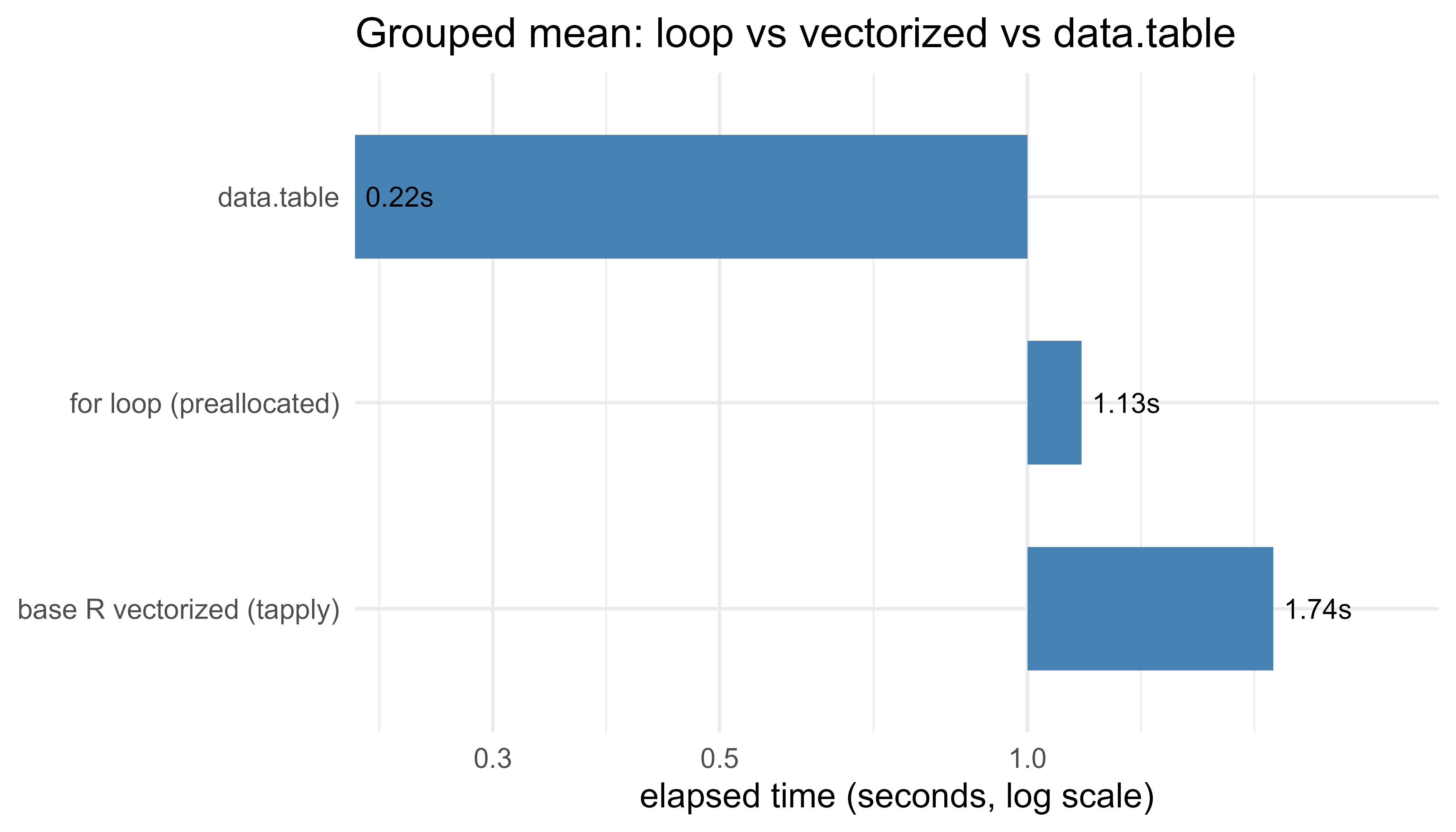
94.7 A Figure: Where the Time Goes
Plotting the timings makes the gap concrete. We use a log scale on the time axis because the differences span more than an order of magnitude. Figure 94.1 shows the elapsed time for each approach, making the order-of-magnitude gap between the loop, tapply, and data.table immediately visible.
Figure 94.1: Elapsed time for a grouped-mean computation on five million rows, by approach. Lower is faster; the time axis is on a log scale.
94.8 Memory and Copying
R’s copy-on-modify model is convenient and a frequent performance trap. The mechanism is reference counting: an object carries a count of how many names point at it, and a modification is done in place only when the count says it is safe (no other name would observe the change). When in doubt the interpreter copies.
You can watch this with tracemem(), which prints a message every time an object is duplicated. Two practical consequences:
Adding or modifying a column of a data frame in a loop can copy the whole frame each time. data.table’s := avoids this by mutating in place.
Passing a large object to a function and modifying it inside copies it, because the argument and the caller’s variable are two names for one object.
The other memory tool is the garbage collector. R allocates from a managed heap and reclaims unreferenced objects automatically; gc() forces a collection and reports memory in use, and the profiler can attribute allocations with Rprof(memory.profiling = TRUE). Excessive allocation, not raw arithmetic, is often the real cost of a slow vectorized pipeline: every intermediate vector is allocated, used once, and discarded, and the allocation plus garbage collection can dominate. Reducing the number of intermediates (or fusing them in compiled code) is then the win.
Tip
tracemem(x) marks an object and prints a one-line message every time R copies it. Wrap a suspicious loop in tracemem/untracemem and watch the console: if you see a copy message on every iteration, you have found a hidden quadratic cost, and that is your cue to preallocate or switch to a data.table and :=.
94.9 Byte Compilation
R compiles function bodies to bytecode for a small register-based virtual machine, which removes some of the parsing and lookup overhead of pure interpretation. Since R 3.4 this is automatic: packages are byte-compiled at install time and ordinary functions are JIT-compiled after a few calls (controlled by compiler::enableJIT). You can compile a function explicitly with compiler::cmpfun.
The realistic expectation: byte compilation helps scalar loop-heavy R code by a modest factor (often well under 2x, and sometimes nothing once the JIT has already compiled the function), and it does almost nothing for code that already spends its time inside vectorized primitives, because the bytecode VM still calls the same C routines. It is free, so there is no reason to avoid it, but it is not a substitute for vectorization. If your code is slow after vectorizing, byte compilation will not rescue it; Rcpp might.
Note
Because the JIT compiler now kicks in automatically after a function has been called a few times, you may see little or no difference from an explicit cmpfun, exactly as in the timing above where both versions land at the same elapsed time. That is the system working as intended, not a failure of the technique.
94.10 BLAS: The Library Under Every Matrix Multiply
Linear algebra in R (matrix products, crossprod, solve, chol, qr, svd, and therefore the internals of lm, glm, ridge and PCA) is dispatched to a BLAS (Basic Linear Algebra Subprograms) and LAPACK library.5 The default that ships with R is a reference implementation that is correct but single-threaded and not cache-optimized. Replacing it with an optimized BLAS (OpenBLAS, Intel MKL, or Apple’s Accelerate) can speed up matrix-heavy work by a large factor with zero code change, because the optimized libraries use blocking for cache locality, vectorized CPU instructions, and multiple cores.
The cost of a dense matrix multiply \(C = AB\) with \(A \in \mathbb{R}^{m\times k}\) and \(B \in \mathbb{R}^{k\times n}\) is \(O(mkn)\) floating-point operations. The reference BLAS does these operations in a naive order with poor cache reuse; an optimized BLAS does the same \(O(mkn)\) flops but partitions the matrices into blocks that fit in cache and keeps the arithmetic units busy, which is where the speedup comes from. You can see which library is active with sessionInfo() (it reports the BLAS/LAPACK paths) or extSoftVersion().
Show code
.libPaths(c("C:/Users/miken/R/library-4.4", .libPaths()))set.seed(7)A<-matrix(rnorm(1500*1500), 1500, 1500)t_mm<-system.time(B<-A%*%A)["elapsed"]blas<-La_library()# path to the active BLAS, or "" for the reference buildcat("BLAS in use:", if(nzchar(blas))blaselse"reference (built-in)", "\n")#> BLAS in use: reference (built-in)cat("1500x1500 matrix multiply elapsed (s):", round(t_mm, 3), "\n")#> 1500x1500 matrix multiply elapsed (s): 2.48
When to use this
If profiling shows your time going into lm, glm, svd, solve, or any large %*%, an optimized BLAS is the highest-leverage fix available, precisely because it speeds up that work with no change to your code. If your time is going into data prep or scalar loops instead, the BLAS is irrelevant and you should look elsewhere.
Practical guidance: if your workload is dominated by large dense linear algebra (large regressions, kernel methods, dimension reduction such as the PCA of Chapter 27), installing an optimized multi-threaded BLAS is usually the single highest-leverage change, and it requires no edits to your R code. Watch for one interaction: a multi-threaded BLAS combined with multi-process parallelism (for example parallel::mclapply over BLAS-heavy tasks, covered in the parallel computing chapter, Chapter 95) can oversubscribe the cores, and you may need to cap BLAS threads (for example via RhpcBLASctl::blas_set_num_threads) so the two layers do not fight.
94.11 Rcpp: When the Loop Cannot Be Vectorized
Some computations are inherently sequential and cannot be expressed as whole-array operations: a recurrence where each value depends on the previous one (an exponential moving average, a custom state machine, a simulation that branches), or a loop with early termination. These are exactly the cases where an R loop is slowest and vectorization does not apply. Rcpp lets you write the hot loop in C++ and call it from R, getting compiled speed for the part that needs it while keeping the rest of the workflow in R.
When to use this
Reach for Rcpp only when the profiler shows a genuinely sequential hot loop (a recurrence, a state machine, a loop with early exit) that no vectorized or data.table form can express, and that loop dominates the runtime. If a vectorized solution exists, it will almost always be simpler and fast enough.
The model is to push only the inner loop into C++. You do not rewrite the program; you replace the one function that the profiler flagged. Rcpp handles the conversion between R vectors and C++ types (NumericVector, IntegerVector) so the boundary is thin. The example below is an exponential moving average, \(s_t = \alpha x_t + (1-\alpha) s_{t-1}\), which is a true recurrence: \(s_t\) needs \(s_{t-1}\), so there is no vectorized form. It is marked eval=FALSE because compiling it needs a C++ toolchain (Rtools on Windows) that the book build does not assume, but it is correct, idiomatic code you can compile with Rcpp::sourceCpp once that toolchain is in place.
Show code
library(Rcpp)cppFunction('NumericVector ema_cpp(NumericVector x, double alpha) { int n = x.size(); NumericVector s(n); if (n == 0) return s; s[0] = x[0]; // seed with the first value for (int t = 1; t < n; ++t) { s[t] = alpha * x[t] + (1.0 - alpha) * s[t-1]; // sequential recurrence } return s;}')# Pure-R equivalent for comparison (this loop cannot be vectorized away).ema_r<-function(x, alpha){n<-length(x); s<-numeric(n)if(n==0)return(s)s[1]<-x[1]for(tin2:n)s[t]<-alpha*x[t]+(1-alpha)*s[t-1]s}set.seed(1)x<-rnorm(1e7)all.equal(ema_cpp(x, 0.1), ema_r(x, 0.1))# TRUE: same numberssystem.time(ema_cpp(x, 0.1))# typically tens of millisecondssystem.time(ema_r(x, 0.1))# typically seconds: 50x-100x slower
For a recurrence like this, Rcpp commonly buys a 50x to 100x speedup over the R loop, because the C++ version pays no per-element interpreter cost and no allocation beyond the single output vector. The trade-off is a compile step, a C++ toolchain (Rtools on Windows), and code that is harder to debug than R. Reach for it last, only after profiling shows a genuinely non-vectorizable hot loop dominates the runtime.
94.12 Practical Guidance, Pitfalls, and When to Use What
A decision order that works in practice is summarized in Table 94.1, which maps each common symptom to the first tool to reach for.
Table 94.1: A diagnosis-to-tool routing guide for R performance work: each symptom points at the first technique to try and a note on what it buys.
Optimizing without profiling. The most common mistake is rewriting the wrong code. Measure first; the bottleneck is usually not where intuition says.
Microbenchmarking noise. A single system.time() on a fast operation is dominated by jitter. Use bench::mark or microbenchmark with replicates, and benchmark realistic input sizes, since the fastest method at \(n = 100\) is often not the fastest at \(n = 10^7\).
Accidental copies. Modifying columns of a data frame in a loop, or passing big objects into functions that mutate them, triggers copies. Use tracemem to catch them, and data.table to avoid them.
Vectorization that allocates too much. Long chains of vectorized operations on huge vectors can be memory-bound from intermediates; sometimes a single compiled pass is both faster and lighter.
Premature Rcpp. C++ adds build complexity and a class of bugs R does not have. If a vectorized or data.table solution exists, prefer it; save Rcpp for true recurrences and other non-vectorizable loops.
Thread oversubscription. A multi-threaded BLAS inside a multi-process parallel map can use more threads than you have cores and slow down. Cap one layer.
The throughline: keep work inside compiled code (vectorized primitives, data.table, optimized BLAS, or your own Rcpp) and out of the interpreter, profile to find where the interpreter is actually running, and stop once the code is fast enough to stop blocking you.
Key idea
Performance work in R is mostly a routing problem. Profile to find the slow step, identify which kind of slowness it is (interpreter overhead, accidental copying, unoptimized linear algebra, or a true sequential loop), and send it to the matching tool in the table above. The cleverness is in the diagnosis, not in the rewrite.
94.13 Further Reading
Wickham, H. (2019). Advanced R, 2nd edition. Chapman and Hall/CRC. Chapters on profiling, performance, and the copy-on-modify model.
Gillespie, C., and Lovelace, R. (2016). Efficient R Programming. O’Reilly. Practical, profiling-driven optimization across the R stack.
Eddelbuettel, D. (2013). Seamless R and C++ Integration with Rcpp. Springer. The reference for Rcpp.
Eddelbuettel, D., and Francois, R. (2011). Rcpp: Seamless R and C++ integration. Journal of Statistical Software. The original Rcpp paper.
Dowle, M., and Srinivasan, A. data.table package vignettes and reference manual. The authoritative source on DT[i, j, by], keys, and :=.
Tierney, L. (2019). A byte code compiler for R. R Project documentation. The design of the R bytecode VM.
Golub, G. H., and Van Loan, C. F. (2013). Matrix Computations, 4th edition. Johns Hopkins University Press. Blocked algorithms and the basis for optimized BLAS.
Chambers, J. M. (2008). Software for Data Analysis: Programming with R. Springer. The language internals behind R’s evaluation model.
The same arithmetic is why a single big bottleneck is good news: if one step is 90% of your runtime (\(p = 0.9\)), speeding it up tenfold cuts total time roughly in half, and there is nowhere else with comparable payoff.↩︎
More precisely, R uses reference counting: an object is duplicated only when more than one name could observe the change. The “as if copied” behavior is what you should reason about; the reference counting is the implementation that sometimes lets R skip the copy. We return to this in the section on memory.↩︎
vapply requires you to declare the type and length of each result, for example vapply(x, f, numeric(1)), so it fails loudly if f ever returns the wrong shape instead of silently producing a list. That safety is worth the extra argument in production code.↩︎
The same trade-off as an index in a relational database: you pay a one-time sorting cost so that every later lookup is cheap. If you filter or join on the same column repeatedly, set a key once with setkey(DT, col) and amortize that cost.↩︎
BLAS is a standardized interface for low-level operations such as matrix multiply; LAPACK is a higher-level library (solvers, decompositions) built on top of it. Several vendors ship optimized implementations of that same interface, which is why you can swap one in without changing any R code.↩︎
Source Code
# High-Performance R {#sec-high-performance-r}```{r}#| include: falsesource("_common.R")```R has a reputation for being slow. Some of that reputation is earned: R is an interpreted, dynamically typed language with copy-on-modify semantics, and a naive R loop can run orders of magnitude slower than the equivalent C. Most of that reputation is avoidable. The same interpreter that runs a slow loop also dispatches to compiled, vectorized primitives and to highly tuned linear algebra libraries, and with a little care you can spend almost all of your runtime inside that compiled code instead of inside the interpreter.This chapter is about making R fast enough that it stays out of your way during a data science or ML workflow: cleaning and reshaping data, engineering features, fitting models, and scoring predictions at volume. The plan is to measure first (profiling with `Rprof` and `profvis`), then attack the usual bottlenecks in order: vectorization, `data.table` for grouped aggregation, memory and copying, the byte compiler, the BLAS that backs every matrix multiply, and finally `Rcpp` for the rare hot loop that genuinely cannot be vectorized. The runnable demo times a hand-written loop against a vectorized version and against `data.table` on simulated data and reports the speedups in a table.By the end you should be able to find the slow part of a pipeline instead of guessing at it, know which of a small set of standard tools fixes each kind of slowness, and recognize the handful of situations where dropping to C++ is actually worth the trouble. The single idea underneath all of it: keep the work inside compiled code and out of the interpreter.::: {.callout-important title="Key idea"}R is fast when it spends its time inside compiled, vectorized routines and slow when it spends its time in the interpreter running one element at a time. Almost every technique in this chapter is a different way to move work from the second place to the first.:::## Where Performance Work FitsIn a modeling project the wall-clock time is rarely spent where you expect. A typical breakdown is: a lot of time in data preparation (joins, group-by aggregations, reshaping), a chunk in the model fit itself (often a `.Call` into compiled code you do not control), and a surprising amount in glue code, the loops and `apply` calls that move data between steps. The model fit is usually already optimized by its package authors. The glue and the data prep are where your own code lives, and that is where speedups are available.The discipline that matters is to optimize in the right order:1. Make it correct. A fast wrong answer is worthless, and rewriting working code for speed risks breaking it.2. Measure where the time goes. Intuition about R bottlenecks is unreliable; profile before changing anything.3. Fix the largest cost first. By Amdahl's law, if a section is 5% of runtime, making it infinitely fast saves at most 5%.4. Stop when it is fast enough. Beyond the point where runtime stops blocking you, further tuning is a hobby, not engineering.Amdahl's law makes the third point precise. If a fraction $p$ of total runtime is sped up by a factor $s$, the overall speedup is$$S = \frac{1}{(1-p) + \tfrac{p}{s}}.$$As $s \to \infty$ the best you can do is $1/(1-p)$. Optimizing a routine that is 10% of runtime ($p = 0.1$) can never give more than an $11\%$ improvement no matter how clever the rewrite, which is why profiling to find the large $p$ comes before any optimization.^[The same arithmetic is why a single big bottleneck is good news: if one step is 90% of your runtime ($p = 0.9$), speeding it up tenfold cuts total time roughly in half, and there is nowhere else with comparable payoff.]::: {.callout-tip}Before you change a line of code for speed, write down what "fast enough" means for this task (a report that must finish overnight, an interactive query that should feel instant). Optimization has no natural stopping point, so the target has to come from outside the code.:::## Why R Loops Are SlowThree properties of the R evaluator explain most of the overhead in interpreted R code. They are worth understanding because each one points at a specific cure, and because once you can name them you stop being surprised by where the time goes.::: {.callout-tip title="Intuition"}Think of the R interpreter as a clerk who, for every single arithmetic operation, has to look up what the symbols mean, check that the inputs are the type they claim to be, find a clean sheet of paper, do the sum, and file the result. For one big batch of numbers that overhead is paid once; for a million scalar operations in a loop it is paid a million times, and the overhead, not the arithmetic, is what you are timing.:::Interpretation and dispatch. Every iteration of an R `for` loop re-enters the interpreter: it looks up the operator (`+`, `[`, etc.), checks the types and classes of its arguments, dispatches to the right method, allocates a result, and returns. For a scalar addition the bookkeeping costs far more than the addition. A vectorized call does this bookkeeping once for the whole vector, then runs a tight C loop over the elements.Dynamic typing. An R numeric vector is a contiguous block of doubles, but a single variable can be reassigned to a character vector at any time, so the interpreter cannot assume types across iterations and must re-check them.Copy-on-modify. R values behave as if copied on assignment.^[More precisely, R uses reference counting: an object is duplicated only when more than one name could observe the change. The "as if copied" behavior is what you should reason about; the reference counting is the implementation that sometimes lets R skip the copy. We return to this in the section on memory.] If you modify a vector inside a loop in a way the interpreter cannot prove is safe to do in place, R allocates a fresh copy. The classic disaster is growing a vector by `x <- c(x, new)` or `x[[length(x)+1]] <- new`: each step may reallocate and copy the whole accumulated result, turning an $O(n)$ task into $O(n^2)$.The single most important habit is to preallocate. Create the result at full size once (`numeric(n)`, `vector("list", n)`) and fill it by index, so the loop does $O(n)$ total work and the interpreter can update in place.::: {.callout-warning}Growing a result with `c()`, `rbind()`, or `append()` inside a loop is the most common accidental performance bug in R. It looks innocent and works fine on small inputs, then quietly becomes quadratic on large ones because each append copies everything accumulated so far. If you must build up a result, collect the pieces in a preallocated list and combine once at the end.:::## Profiling: Measure Before You ChangeR ships with a sampling profiler. `Rprof()` writes the current call stack to a file many times per second; `summaryRprof()` aggregates how often each function was on the stack, which approximates where time is spent. The `profvis` package wraps the same mechanism in an interactive flame graph that lines up time with source code. Sampling profilers are cheap and do not need you to annotate the code, but they only see functions that the interpreter records on the stack, so very short calls can be missed.The two summaries to read are `self` time (spent inside a function, excluding its callees) and `total` time (including callees). High self time points at the function to rewrite; high total time with low self time points at an expensive child.::: {.callout-note}A sampling profiler tells you where time goes, not why. It is the right tool for locating the bottleneck. To then compare two candidate rewrites of that bottleneck, switch to a benchmarking tool (`system.time` for a quick number, `bench::mark` or `microbenchmark` for careful timing with replicates).:::```{r hpr-rprof, eval=TRUE}.libPaths(c("C:/Users/miken/R/library-4.4", .libPaths()))set.seed(1)slow_sum_of_squares <-function(n) { s <-0for (i inseq_len(n)) s <- s + i^2# scalar work, one interpreter trip per i s}tmp <-tempfile(fileext =".out")Rprof(tmp, interval =0.005)invisible(slow_sum_of_squares(2e6))Rprof(NULL)prof <-summaryRprof(tmp)head(prof$by.self, 4)```For interactive use you would wrap the same call in `profvis::profvis({ slow_sum_of_squares(2e6) })` and read the flame graph. For a single timing number, `system.time()` (or `bench::mark()` for careful microbenchmarks with multiple replicates) is enough; for finding the hot spot in a larger pipeline, reach for the profiler.## VectorizationVectorization replaces an explicit element-by-element loop with a single call to a function that loops in C. The arithmetic done is identical; what disappears is the per-element interpreter overhead. Summing squares vectorizes to `sum(x^2)`: `x^2` runs one C loop to square every element, and `sum` runs one C loop to add them, with two interpreter calls total instead of $n$.::: {.callout-tip title="When to use this"}Reach for vectorization first whenever a loop's body does the same scalar operation to each element independently, with no element depending on a previous one. That description covers most arithmetic, filtering, and conditional assignment, and it is exactly where R loops are slowest and vectorization wins biggest.:::Vectorization is not only about speed. Vectorized code is usually shorter and closer to the math, which makes it easier to read and harder to get wrong. The mental shift is to think in whole arrays: instead of "for each row, do this," ask "what operation maps the input column to the output column." Filtering becomes logical indexing (`x[x > 0]`), conditional assignment becomes `ifelse()` or `pmax()/pmin()`, and cumulative quantities become `cumsum()`, `cumprod()`, `cummax()`. The `apply` family (`vapply`, `lapply`, `Map`) is not vectorization in this sense, it is still an R-level loop, but it is clearer than a hand-written loop and `vapply` is type-safe.^[`vapply` requires you to declare the type and length of each result, for example `vapply(x, f, numeric(1))`, so it fails loudly if `f` ever returns the wrong shape instead of silently producing a list. That safety is worth the extra argument in production code.]A caution: vectorized operations allocate intermediate vectors. `sum(x^2)` materializes the full `x^2` before summing, which costs memory proportional to the input. For most data this is fine; for very large vectors the memory traffic can matter, and that is one place a compiled one-pass loop (via `Rcpp`) wins.## data.table: Fast Grouped AggregationThe most common heavy data step in practice is a group-by aggregation: split rows into groups, compute a summary per group, combine. `data.table` is built for exactly this. Three design choices make it fast.::: {.callout-tip title="Intuition"}A grouped aggregation is conceptually a database `GROUP BY`. `data.table` treats it that way, doing the grouping and the per-group reduction in one pass of compiled C, rather than splitting the data into thousands of little R objects and looping over them.:::Modification by reference. The `:=` operator and `set()` update columns in place, without the copy that a base R `df$col <- ...` or a `dplyr::mutate` may trigger. This avoids duplicating a large table just to add or change one column.Optimized grouping. The `DT[i, j, by]` syntax computes the grouping once and runs the aggregation `j` per group in compiled C, including special fast paths (called GForce) for common reducers such as `sum`, `mean`, `min`, `max`, and `.N`.Keys and indices. Setting a key sorts the table and lets joins and subsets use binary search ($O(\log n)$) instead of a full scan ($O(n)$).^[The same trade-off as an index in a relational database: you pay a one-time sorting cost so that every later lookup is cheap. If you filter or join on the same column repeatedly, set a key once with `setkey(DT, col)` and amortize that cost.]The mental model for `DT[i, j, by]` is "take rows `i`, compute `j`, grouped by `by`," which maps directly onto SQL's `WHERE`, `SELECT`, and `GROUP BY`. For data that fits in memory this is typically the fastest grouped aggregation available in R, and the syntax stays compact as the operations stack up.## Timing Demo: Loop vs Vectorized vs data.tableThe task: simulate a large data set with a numeric value and a grouping factor, then compute the mean of the value within each group. We time three approaches that all return the same per-group means: a hand-written loop over groups, a base R vectorized approach (`tapply`, which dispatches to a compiled grouped sum), and `data.table`. `system.time()` reports elapsed seconds; we collect them into a comparison table.```{r hpr-timing, eval=TRUE}.libPaths(c("C:/Users/miken/R/library-4.4", .libPaths()))suppressPackageStartupMessages(library(data.table))set.seed(42)n <-5e6# number of rowsng <-50000# number of groupsg <-sample.int(ng, n, replace =TRUE) # group id per rowx <-rnorm(n) # value per row# 1) Hand-written loop with PREALLOCATED accumulators (the right way to loop).loop_group_means <-function(g, x, ng) { sums <-numeric(ng) counts <-integer(ng)for (i inseq_along(x)) { gi <- g[i] sums[gi] <- sums[gi] + x[i] counts[gi] <- counts[gi] +1L } sums / counts}t_loop <-system.time(m_loop <-loop_group_means(g, x, ng))# 2) Base R vectorized: tapply runs the grouping in compiled code.t_vec <-system.time(m_vec <-tapply(x, g, mean))# 3) data.table: grouped mean with the GForce fast path.DT <-data.table(g = g, x = x)t_dt <-system.time(m_dt <- DT[, .(m =mean(x)), by = g])# Confirm all three agree (reorder data.table result by group id).setorder(m_dt, g)stopifnot(max(abs(m_loop -as.numeric(m_vec))) <1e-8,max(abs(m_dt$m -as.numeric(m_vec))) <1e-8)timing <-data.frame(approach =c("for loop (preallocated)", "base R vectorized (tapply)", "data.table"),elapsed_sec =c(t_loop["elapsed"], t_vec["elapsed"], t_dt["elapsed"]),row.names =NULL)timing$speedup_vs_loop <-round(timing$elapsed_sec[1] / timing$elapsed_sec, 1)timing$elapsed_sec <-round(timing$elapsed_sec, 3)timing```The exact numbers depend on the machine, but the robust conclusion is that `data.table` is the fastest by a wide margin and scales best as the number of groups and rows grows. The base R `tapply` runs its reduction in compiled code but pays to build and sort a factor with one level per group, which with tens of thousands of groups can make it no faster, or even slower, than the preallocated loop. That is itself a useful lesson: "vectorized" is not automatically "fast" when a hidden step (here, factor construction over many levels) scales with the data. The preallocated loop, meanwhile, is $O(n)$ rather than $O(n^2)$ precisely because the accumulators were created once and filled by index; the same loop written by growing a vector would be far worse. The dedicated grouped engine in `data.table` avoids both the per-row interpreter cost and the factor overhead, which is why it wins.::: {.callout-warning}Do not read "vectorized" as a synonym for "fast." A vectorized call moves the visible loop into C, but it can still hide a step that scales badly with the data, as `tapply` does here by building a factor with one level per group. Always benchmark on realistic input sizes rather than trusting the label.:::## A Figure: Where the Time GoesPlotting the timings makes the gap concrete. We use a log scale on the time axis because the differences span more than an order of magnitude. @fig-high-performance-r-timing-bars shows the elapsed time for each approach, making the order-of-magnitude gap between the loop, `tapply`, and `data.table` immediately visible.```{r fig-high-performance-r-timing-bars, eval=TRUE, fig.width=7, fig.height=4, fig.cap="Elapsed time for a grouped-mean computation on five million rows, by approach. Lower is faster; the time axis is on a log scale."}.libPaths(c("C:/Users/miken/R/library-4.4", .libPaths()))suppressPackageStartupMessages(library(ggplot2))timing$approach <-factor(timing$approach, levels = timing$approach[order(-timing$elapsed_sec)])ggplot(timing, aes(x = approach, y = elapsed_sec)) +geom_col(width =0.6, fill ="steelblue") +geom_text(aes(label =paste0(elapsed_sec, "s")), hjust =-0.15, size =3.4) +scale_y_log10(expand =expansion(mult =c(0, 0.18))) +coord_flip() +labs(x =NULL, y ="elapsed time (seconds, log scale)",title ="Grouped mean: loop vs vectorized vs data.table") +theme_minimal(base_size =12)```## Memory and CopyingR's copy-on-modify model is convenient and a frequent performance trap. The mechanism is reference counting: an object carries a count of how many names point at it, and a modification is done in place only when the count says it is safe (no other name would observe the change). When in doubt the interpreter copies.You can watch this with `tracemem()`, which prints a message every time an object is duplicated. Two practical consequences:- Adding or modifying a column of a data frame in a loop can copy the whole frame each time. `data.table`'s `:=` avoids this by mutating in place.- Passing a large object to a function and modifying it inside copies it, because the argument and the caller's variable are two names for one object.The other memory tool is the garbage collector. R allocates from a managed heap and reclaims unreferenced objects automatically; `gc()` forces a collection and reports memory in use, and the profiler can attribute allocations with `Rprof(memory.profiling = TRUE)`. Excessive allocation, not raw arithmetic, is often the real cost of a slow vectorized pipeline: every intermediate vector is allocated, used once, and discarded, and the allocation plus garbage collection can dominate. Reducing the number of intermediates (or fusing them in compiled code) is then the win.::: {.callout-tip}`tracemem(x)` marks an object and prints a one-line message every time R copies it. Wrap a suspicious loop in `tracemem`/`untracemem` and watch the console: if you see a copy message on every iteration, you have found a hidden quadratic cost, and that is your cue to preallocate or switch to a `data.table` and `:=`.:::## Byte CompilationR compiles function bodies to bytecode for a small register-based virtual machine, which removes some of the parsing and lookup overhead of pure interpretation. Since R 3.4 this is automatic: packages are byte-compiled at install time and ordinary functions are JIT-compiled after a few calls (controlled by `compiler::enableJIT`). You can compile a function explicitly with `compiler::cmpfun`.```{r hpr-bytecomp, eval=TRUE}.libPaths(c("C:/Users/miken/R/library-4.4", .libPaths()))library(compiler)f_interp <-function(n) { s <-0; for (i inseq_len(n)) s <- s +sqrt(i); s }f_comp <-cmpfun(f_interp)t_i <-system.time(for (r in1:5) f_interp(1e6))["elapsed"]t_c <-system.time(for (r in1:5) f_comp(1e6))["elapsed"]data.frame(version =c("interpreted (JIT off-path)", "explicitly compiled"),elapsed =round(c(t_i, t_c), 3), row.names =NULL)```The realistic expectation: byte compilation helps scalar loop-heavy R code by a modest factor (often well under 2x, and sometimes nothing once the JIT has already compiled the function), and it does almost nothing for code that already spends its time inside vectorized primitives, because the bytecode VM still calls the same C routines. It is free, so there is no reason to avoid it, but it is not a substitute for vectorization. If your code is slow after vectorizing, byte compilation will not rescue it; `Rcpp` might.::: {.callout-note}Because the JIT compiler now kicks in automatically after a function has been called a few times, you may see little or no difference from an explicit `cmpfun`, exactly as in the timing above where both versions land at the same elapsed time. That is the system working as intended, not a failure of the technique.:::## BLAS: The Library Under Every Matrix MultiplyLinear algebra in R (matrix products, `crossprod`, `solve`, `chol`, `qr`, `svd`, and therefore the internals of `lm`, `glm`, ridge and PCA) is dispatched to a BLAS (Basic Linear Algebra Subprograms) and LAPACK library.^[BLAS is a standardized interface for low-level operations such as matrix multiply; LAPACK is a higher-level library (solvers, decompositions) built on top of it. Several vendors ship optimized implementations of that same interface, which is why you can swap one in without changing any R code.] The default that ships with R is a reference implementation that is correct but single-threaded and not cache-optimized. Replacing it with an optimized BLAS (OpenBLAS, Intel MKL, or Apple's Accelerate) can speed up matrix-heavy work by a large factor with zero code change, because the optimized libraries use blocking for cache locality, vectorized CPU instructions, and multiple cores.The cost of a dense matrix multiply $C = AB$ with $A \in \mathbb{R}^{m\times k}$ and $B \in \mathbb{R}^{k\times n}$ is $O(mkn)$ floating-point operations. The reference BLAS does these operations in a naive order with poor cache reuse; an optimized BLAS does the same $O(mkn)$ flops but partitions the matrices into blocks that fit in cache and keeps the arithmetic units busy, which is where the speedup comes from. You can see which library is active with `sessionInfo()` (it reports the BLAS/LAPACK paths) or `extSoftVersion()`.```{r hpr-blas, eval=TRUE}.libPaths(c("C:/Users/miken/R/library-4.4", .libPaths()))set.seed(7)A <-matrix(rnorm(1500*1500), 1500, 1500)t_mm <-system.time(B <- A %*% A)["elapsed"]blas <-La_library() # path to the active BLAS, or "" for the reference buildcat("BLAS in use:", if (nzchar(blas)) blas else"reference (built-in)", "\n")cat("1500x1500 matrix multiply elapsed (s):", round(t_mm, 3), "\n")```::: {.callout-tip title="When to use this"}If profiling shows your time going into `lm`, `glm`, `svd`, `solve`, or any large `%*%`, an optimized BLAS is the highest-leverage fix available, precisely because it speeds up that work with no change to your code. If your time is going into data prep or scalar loops instead, the BLAS is irrelevant and you should look elsewhere.:::Practical guidance: if your workload is dominated by large dense linear algebra (large regressions, kernel methods, dimension reduction such as the PCA of @sec-dimension-reduction), installing an optimized multi-threaded BLAS is usually the single highest-leverage change, and it requires no edits to your R code. Watch for one interaction: a multi-threaded BLAS combined with multi-process parallelism (for example `parallel::mclapply` over BLAS-heavy tasks, covered in the parallel computing chapter, @sec-parallel-computing) can oversubscribe the cores, and you may need to cap BLAS threads (for example via `RhpcBLASctl::blas_set_num_threads`) so the two layers do not fight.## Rcpp: When the Loop Cannot Be VectorizedSome computations are inherently sequential and cannot be expressed as whole-array operations: a recurrence where each value depends on the previous one (an exponential moving average, a custom state machine, a simulation that branches), or a loop with early termination. These are exactly the cases where an R loop is slowest and vectorization does not apply. `Rcpp` lets you write the hot loop in C++ and call it from R, getting compiled speed for the part that needs it while keeping the rest of the workflow in R.::: {.callout-tip title="When to use this"}Reach for `Rcpp` only when the profiler shows a genuinely sequential hot loop (a recurrence, a state machine, a loop with early exit) that no vectorized or `data.table` form can express, and that loop dominates the runtime. If a vectorized solution exists, it will almost always be simpler and fast enough.:::The model is to push only the inner loop into C++. You do not rewrite the program; you replace the one function that the profiler flagged. `Rcpp` handles the conversion between R vectors and C++ types (`NumericVector`, `IntegerVector`) so the boundary is thin. The example below is an exponential moving average, $s_t = \alpha x_t + (1-\alpha) s_{t-1}$, which is a true recurrence: $s_t$ needs $s_{t-1}$, so there is no vectorized form. It is marked `eval=FALSE` because compiling it needs a C++ toolchain (Rtools on Windows) that the book build does not assume, but it is correct, idiomatic code you can compile with `Rcpp::sourceCpp` once that toolchain is in place.```{r hpr-rcpp, eval=FALSE}library(Rcpp)cppFunction('NumericVector ema_cpp(NumericVector x, double alpha) { int n = x.size(); NumericVector s(n); if (n == 0) return s; s[0] = x[0]; // seed with the first value for (int t = 1; t < n; ++t) { s[t] = alpha * x[t] + (1.0 - alpha) * s[t-1]; // sequential recurrence } return s;}')# Pure-R equivalent for comparison (this loop cannot be vectorized away).ema_r <-function(x, alpha) { n <-length(x); s <-numeric(n)if (n ==0) return(s) s[1] <- x[1]for (t in2:n) s[t] <- alpha * x[t] + (1- alpha) * s[t -1] s}set.seed(1)x <-rnorm(1e7)all.equal(ema_cpp(x, 0.1), ema_r(x, 0.1)) # TRUE: same numberssystem.time(ema_cpp(x, 0.1)) # typically tens of millisecondssystem.time(ema_r(x, 0.1)) # typically seconds: 50x-100x slower```For a recurrence like this, `Rcpp` commonly buys a 50x to 100x speedup over the R loop, because the C++ version pays no per-element interpreter cost and no allocation beyond the single output vector. The trade-off is a compile step, a C++ toolchain (Rtools on Windows), and code that is harder to debug than R. Reach for it last, only after profiling shows a genuinely non-vectorizable hot loop dominates the runtime.## Practical Guidance, Pitfalls, and When to Use WhatA decision order that works in practice is summarized in @tbl-high-performance-r-decision-order, which maps each common symptom to the first tool to reach for.| Symptom | First thing to try | Notes ||---|---|---|| Don't know where time goes |`profvis` / `Rprof`| Always profile before optimizing || Explicit element loop over a vector | Vectorize (`sum`, `ifelse`, `cumsum`, `[`) | Identical math, loop moves into C || Growing an object in a loop | Preallocate (`numeric(n)`, fill by index) | Fixes accidental $O(n^2)$ || Group-by / join on a big table |`data.table` (`DT[i, j, by]`, keys) | In-place `:=`, GForce reducers || Large dense linear algebra (`lm`, PCA, kernels) | Optimized BLAS (OpenBLAS / MKL) | No code change, multi-threaded || Scalar loop, already minimal |`compiler::cmpfun` (often automatic) | Modest gain, free || Sequential recurrence / early exit |`Rcpp` hot loop | Last resort, big gain when it applies |: A diagnosis-to-tool routing guide for R performance work: each symptom points at the first technique to try and a note on what it buys. {#tbl-high-performance-r-decision-order}Pitfalls to watch:- Optimizing without profiling. The most common mistake is rewriting the wrong code. Measure first; the bottleneck is usually not where intuition says.- Microbenchmarking noise. A single `system.time()` on a fast operation is dominated by jitter. Use `bench::mark` or `microbenchmark` with replicates, and benchmark realistic input sizes, since the fastest method at $n = 100$ is often not the fastest at $n = 10^7$.- Accidental copies. Modifying columns of a data frame in a loop, or passing big objects into functions that mutate them, triggers copies. Use `tracemem` to catch them, and `data.table` to avoid them.- Vectorization that allocates too much. Long chains of vectorized operations on huge vectors can be memory-bound from intermediates; sometimes a single compiled pass is both faster and lighter.- Premature `Rcpp`. C++ adds build complexity and a class of bugs R does not have. If a vectorized or `data.table` solution exists, prefer it; save `Rcpp` for true recurrences and other non-vectorizable loops.- Thread oversubscription. A multi-threaded BLAS inside a multi-process parallel map can use more threads than you have cores and slow down. Cap one layer.The throughline: keep work inside compiled code (vectorized primitives, `data.table`, optimized BLAS, or your own `Rcpp`) and out of the interpreter, profile to find where the interpreter is actually running, and stop once the code is fast enough to stop blocking you.::: {.callout-important title="Key idea"}Performance work in R is mostly a routing problem. Profile to find the slow step, identify which kind of slowness it is (interpreter overhead, accidental copying, unoptimized linear algebra, or a true sequential loop), and send it to the matching tool in the table above. The cleverness is in the diagnosis, not in the rewrite.:::## Further Reading- Wickham, H. (2019). *Advanced R*, 2nd edition. Chapman and Hall/CRC. Chapters on profiling, performance, and the copy-on-modify model.- Gillespie, C., and Lovelace, R. (2016). *Efficient R Programming*. O'Reilly. Practical, profiling-driven optimization across the R stack.- Eddelbuettel, D. (2013). *Seamless R and C++ Integration with Rcpp*. Springer. The reference for `Rcpp`.- Eddelbuettel, D., and Francois, R. (2011). Rcpp: Seamless R and C++ integration. *Journal of Statistical Software*. The original Rcpp paper.- Dowle, M., and Srinivasan, A. *data.table* package vignettes and reference manual. The authoritative source on `DT[i, j, by]`, keys, and `:=`.- Tierney, L. (2019). A byte code compiler for R. R Project documentation. The design of the R bytecode VM.- Golub, G. H., and Van Loan, C. F. (2013). *Matrix Computations*, 4th edition. Johns Hopkins University Press. Blocked algorithms and the basis for optimized BLAS.- Chambers, J. M. (2008). *Software for Data Analysis: Programming with R*. Springer. The language internals behind R's evaluation model.