Most production data science no longer runs against a CSV on a laptop. The data lives in object storage, in a managed warehouse, or behind an API, and the compute that touches it runs on a rented machine somewhere else. This chapter is about how to reach that data and that compute from R, what the cost and performance trade-offs are, and how to write code that does not embed secrets or break when the dataset grows past memory.
The focus is practical. The cloud chunks are marked eval=FALSE because this book builds without cloud credentials, but they are written to be correct and current so a reader with an account can run them. The one fully runnable demonstration is a small base-R abstraction that mirrors an object-store interface against a local directory, which teaches the mental model behind every cloud SDK.
105.1 Where this fits in a modern ML/AI workflow
A typical workflow has three layers that used to live on one machine and now live in three different services:
Storage: raw and processed data sits in object storage (Amazon S3, Google Cloud Storage, Azure Blob). Object storage is cheap, durable, and effectively unbounded, but it is a key-value store, not a filesystem, and not a query engine.
Query and transform: structured analytics runs in a warehouse (BigQuery, Amazon Redshift, Snowflake) or a query engine over files (DuckDB, Spark). You push the computation to the data instead of pulling the data to R.
Compute: model training and batch scoring run on rented CPU or GPU instances, sometimes orchestrated by a scheduler. R is often the client that submits the job and collects the result, not the thing doing the heavy lifting.
The single most important habit is to move computation toward the data. Pulling a 200 GB table into R to compute a group mean wastes network, memory, and money. Issuing a GROUP BY to the warehouse and pulling back a few hundred rows is the same answer for a tiny fraction of the cost. The rest of this chapter is variations on that theme.
Key idea
Push the reduction to where the data lives, and transport only the small result back to R. Almost every recommendation in this chapter follows from that one sentence.
105.1.1 The cost model you are actually optimizing
It helps to write the total cost of a job as a sum of three terms:
where \(p_s\) is a per-gigabyte-month price, \(B\) is bytes stored, and \(t\) is months. Transfer cost is driven by data leaving a region or a cloud (egress),
with \(p_e\) the egress price per gigabyte, \(B_{\text{out}}\) the bytes read out, \(p_r\) the per-request price, and \(N_{\text{req}}\) the number of API calls. Compute cost for a warehouse query is often billed on bytes scanned,
where \(p_q\) is a per-terabyte-scanned price and \(B_{\text{scan}}\) is bytes the engine read to answer the query.1 Two design choices fall straight out of these equations. First, columnar formats and partition pruning shrink \(B_{\text{scan}}\), so they cut the dominant term for analytics. Second, keeping storage and compute in the same region drives \(B_{\text{out}}\) toward zero, because in-region reads are usually free. A surprising fraction of real cloud bills is egress and request count, not storage.
Warning
The term that surprises people on their first cloud bill is usually \(C_{\text{transfer}}\), not \(C_{\text{store}}\). Storing a terabyte for a month is cheap; reading it back across a region boundary or out to the public internet can cost more than storing it for a year. When a bill looks wrong, check egress first.
105.2 Object storage from R
Object storage exposes a flat namespace: a bucket holds objects, each addressed by a key (a string that may contain slashes so it looks like a path). There are no real directories. Listing “a folder” is really listing all keys with a common prefix. The core operations are small: put an object, get an object, list keys under a prefix, delete an object, and check existence.
Intuition
Think of a bucket as one giant hash map from string keys to blobs of bytes, not as a tree of folders. The slashes in datasets/2025/events.parquet are just characters in the key. The console draws them as folders for your comfort, but the storage layer never moves up or down a directory because there is no directory to move through.
The main R interfaces are paws (a generated AWS SDK covering S3 and much else), googleCloudStorageR for GCS, and AzureStor for Azure Blob. Below is idiomatic paws code for the five core operations. It will not run here because there are no credentials, but it is the shape you will use.
Show code
library(paws)# Credentials are read from the standard chain: environment variables,# ~/.aws/credentials, or an instance/role profile. Never hard-code keys.s3<-paws::s3()bucket<-"my-ml-bucket"# PUT: upload a serialized R objectsaveRDS(mtcars, "mtcars.rds")s3$put_object( Bucket =bucket, Key ="datasets/mtcars.rds", Body =readBin("mtcars.rds", "raw", n =file.size("mtcars.rds")))# LIST: enumerate keys under a prefix (note: paginated, max 1000 per call)listing<-s3$list_objects_v2(Bucket =bucket, Prefix ="datasets/")vapply(listing$Contents, function(o)o$Key, character(1))# EXISTS: a head request is cheap and avoids downloading the bodyexists_obj<-tryCatch({s3$head_object(Bucket =bucket, Key ="datasets/mtcars.rds")TRUE}, error =function(e)FALSE)# GET: download to a raw vector, then deserializeobj<-s3$get_object(Bucket =bucket, Key ="datasets/mtcars.rds")tmp<-tempfile(fileext =".rds")writeBin(obj$Body, tmp)restored<-readRDS(tmp)# DELETEs3$delete_object(Bucket =bucket, Key ="datasets/mtcars.rds")
The equivalent in googleCloudStorageR is higher level because it has explicit upload and download helpers:
Show code
library(googleCloudStorageR)# Auth via a service-account JSON key referenced by an env var, not a literal path in code.gcs_auth(json_file =Sys.getenv("GCS_AUTH_FILE"))gcs_global_bucket("my-ml-bucket")gcs_upload(mtcars, name ="datasets/mtcars.rds")# PUTobjs<-gcs_list_objects(prefix ="datasets/")# LISTrestored<-gcs_get_object("datasets/mtcars.rds", # GET saveToDisk =tempfile(), overwrite =TRUE)gcs_delete_object("datasets/mtcars.rds")# DELETE
And Azure Blob through AzureStor:
Show code
library(AzureStor)endp<-storage_endpoint("https://myaccount.blob.core.windows.net", key =Sys.getenv("AZURE_STORAGE_KEY"))cont<-storage_container(endp, "my-ml-container")storage_upload(cont, src ="mtcars.rds", dest ="datasets/mtcars.rds")# PUTlist_storage_files(cont, dir ="datasets")# LISTstorage_download(cont, src ="datasets/mtcars.rds", dest =tempfile())# GETdelete_storage_file(cont, "datasets/mtcars.rds")# DELETE
Across all three providers the interface is the same five verbs over a key-value store. Once you internalize that, switching clouds is mostly renaming functions.
Note
The body of an S3 object comes back as a raw byte vector, which is why the paws example writes it to a temporary file before readRDS(). The higher-level GCS and Azure helpers hide that step behind a saveToDisk/dest argument, but underneath they are doing the same thing.
105.2.1 File formats matter more than the SDK
What you store under those keys decides your query cost. The choice is usually between a row-oriented text format (CSV) and a columnar binary format (Parquet); the formats themselves are treated more fully in Chapter 101.2 Columnar storage lets an engine read only the columns a query touches, and it compresses far better because values within a column share a type and a distribution.
A back-of-the-envelope model: if a query needs \(c\) of \(p\) columns and the columnar format compresses by factor \(\rho\), the bytes scanned drop roughly by
For a wide table where a query touches a few columns, this is often a 10x to 100x reduction, which maps directly onto the \(C_{\text{compute}} = p_q \cdot B_{\text{scan}}\) term above. In R you would write Parquet with arrow:
Show code
library(arrow)# Write a partitioned Parquet dataset directly to S3.# Partitioning by a frequently filtered column lets the reader skip whole files.arrow::write_dataset( dataset =my_data_frame, path ="s3://my-ml-bucket/datasets/events/", format ="parquet", partitioning =c("year", "month"))# Read back lazily: filters and column selection are pushed down,# so only the needed partitions and columns are fetched.ds<-arrow::open_dataset("s3://my-ml-bucket/datasets/events/")library(dplyr)result<-ds|>filter(year==2025, month==6)|>select(user_id, amount)|>group_by(user_id)|>summarise(total =sum(amount))|>collect()# only this line pulls data into R
105.3 Cloud databases and warehouses from R
A warehouse is a managed SQL engine that separates storage from compute and scales the compute elastically. From R, the standard route is the DBI interface plus a driver package, so the same R code talks to BigQuery, Redshift, Snowflake, or a local SQLite by swapping the connection object.
Intuition
DBI is to databases what a wall socket is to appliances. Your R code (the appliance) plugs into a standard interface; the driver package (the plug) handles whatever the specific warehouse expects behind the wall. Change the warehouse and you change the plug, not the appliance.
Show code
library(DBI)library(bigrquery)# BigQuery driver implementing the DBI genericcon<-dbConnect(bigrquery::bigquery(), project =Sys.getenv("GCP_PROJECT"), dataset ="analytics")# Push the aggregation to the warehouse; pull back only the summary.res<-dbGetQuery(con, " SELECT user_id, SUM(amount) AS total FROM analytics.events WHERE event_date >= '2025-01-01' GROUP BY user_id")dbDisconnect(con)
The same pattern with Redshift or Snowflake just changes the driver:
Show code
library(DBI)# Redshift speaks the PostgreSQL wire protocol, so RPostgres works.con_rs<-dbConnect(RPostgres::Redshift(), host =Sys.getenv("REDSHIFT_HOST"), port =5439, dbname ="warehouse", user =Sys.getenv("REDSHIFT_USER"), password =Sys.getenv("REDSHIFT_PASSWORD"))# Snowflake via the odbc package and the Snowflake ODBC driver.con_sf<-dbConnect(odbc::odbc(), Driver ="SnowflakeDSIIDriver", Server =Sys.getenv("SNOWFLAKE_ACCOUNT"), UID =Sys.getenv("SNOWFLAKE_USER"), PWD =Sys.getenv("SNOWFLAKE_PASSWORD"), Warehouse ="COMPUTE_WH", Database ="ANALYTICS")
The most useful pattern for analysts is to let dbplyr translate dplyr verbs into SQL so you never hand-write the query, and so the computation stays in the warehouse until you call collect():
Show code
library(dplyr)library(dbplyr)events<-tbl(con, "events")# a lazy reference, no data moved yetsummary_tbl<-events|>filter(event_date>="2025-01-01")|>group_by(user_id)|>summarise(total =sum(amount), n =n())show_query(summary_tbl)# inspect the generated SQLlocal_result<-collect(summary_tbl)# execute remotely, fetch the small result
The discipline is identical to object storage: do the reduction remotely, transport the small thing.
Tip
The lazy reference events looks like a data frame but holds no rows. Nothing runs until collect(). Get in the habit of calling show_query() before collect() so you can confirm the filter and the GROUP BY were pushed to the warehouse, not quietly applied in R after a full download.
105.4 Comparison of the main options
Table 105.1 summarizes the storage and query options discussed, with the R package you would reach for and the cost driver to watch. Prices change constantly, so the table gives the billing model, not numbers.
Table 105.1: Storage and query options for cloud data work from R, with the primary R interface, the billing driver to watch, and the workload each option suits best.
Service
Type
Primary R interface
Billing driver
Best for
Amazon S3
Object storage
paws
Storage GB-month, requests, egress
Raw data lake, model artifacts
Google Cloud Storage
Object storage
googleCloudStorageR
Storage GB-month, operations, egress
Same, GCP-native pipelines
Azure Blob
Object storage
AzureStor
Storage GB-month, operations, egress
Same, Azure-native pipelines
BigQuery
Serverless warehouse
bigrquery + DBI
Bytes scanned per query
Ad hoc analytics, no cluster to manage
Amazon Redshift
Provisioned warehouse
RPostgres + DBI
Cluster node-hours
Steady heavy workloads on AWS
Snowflake
Elastic warehouse
odbc + DBI
Warehouse credits (compute-seconds)
Bursty multi-team analytics
Parquet on object store
File + query engine
arrow, duckdb
Bytes scanned (engine) + storage
Cheap columnar lakehouse queries
A rough rule: object storage is where bytes rest, a warehouse or query engine is where bytes are reduced, and the choice among warehouses is mostly about whether your load is steady (provisioned) or bursty (serverless or elastic).
105.5 Credentials and secrets
A credential, an access key or password that proves you may read a bucket or query a warehouse, is the most dangerous thing in a data pipeline, because a leaked one gives a stranger your access and your bill. The cardinal rule is that secrets never appear in source code, in notebooks, or in version control. The mechanisms, in rough order of preference:
Identity attached to the compute (an IAM role on an EC2 instance, a workload identity on a GCP VM, a managed identity on Azure). The SDK picks up short-lived credentials automatically and there is nothing to leak.
A secrets manager (AWS Secrets Manager, GCP Secret Manager, Azure Key Vault, or HashiCorp Vault) that the application reads at run time.
Environment variables set by the deployment, read in R with Sys.getenv().
A local config file outside the repo, such as ~/.aws/credentials or a service-account JSON, referenced by path through an env var.
In R, Sys.getenv("NAME") returns "" for an unset variable, so guard against silent misconfiguration:
Show code
get_required_env<-function(name){val<-Sys.getenv(name, unset =NA_character_)if(is.na(val)||!nzchar(val)){stop(sprintf("Required environment variable %s is not set", name), call. =FALSE)}val}aws_key<-get_required_env("AWS_ACCESS_KEY_ID")
For local development, the .Renviron file holds variables outside the script, and the keyring package stores secrets in the operating system credential store. Whatever you do, add credential files to .gitignore and prefer attached identity in production so there is no long-lived key to rotate or lose.
Warning
A secret committed to git is compromised the moment the commit is pushed, and deleting it later does not help because it lives forever in the repository history. Treat any key that touches version control as already leaked: rotate it immediately rather than hoping nobody noticed.
105.6 Remote compute
So far the data was too big for the laptop but the computation was light. Sometimes the reverse is true: the dataset fits, but training the model is what overwhelms one machine. When the model, not just the data, is too big for the laptop, the compute moves too. The common patterns from R:
Submit a job to a managed batch service or a cluster scheduler and poll for completion. R is the client.
Use a distributed engine such as Spark through sparklyr, which translates dplyr and MLlib calls into work on the cluster (covered in depth in Chapter 96).
Train on a remote GPU instance with keras/tensorflow or torch, where R drives the training loop on hardware you rented (see Chapter 92).
A sparklyr sketch, where the data and the model fit both stay on the cluster:
The decision of whether to scale up (a bigger single machine) or scale out (many machines) is governed by how the work parallelizes. If a job splits into \(n\) independent tasks of which a fraction \(s\) must run serially, Amdahl’s law bounds the speedup from \(k\) workers at
which approaches \(1/s\) as \(k \to \infty\). The practical reading: distributing only pays when the serial fraction \(s\) is small and the per-task overhead is much smaller than the per-task work. Many “embarrassingly parallel” jobs (scoring rows, fitting independent models per group) have \(s\) near zero and scale almost linearly; iterative algorithms with a synchronization barrier each step do not.
When to use this
Reach for a distributed engine like Spark only after a single large instance is genuinely too small. A 64-core machine with a few hundred gigabytes of RAM handles a lot, and it has no network shuffle, no cluster to babysit, and no serial-fraction penalty. Scale up first; scale out when up runs out.
105.7 A runnable demo: a local store that mirrors an object-store interface
The cleanest way to understand cloud SDKs is to build the abstraction yourself against a local directory. The five verbs (put, get, list, exists, delete) and the flat key namespace are exactly what S3, GCS, and Blob expose. The function factory below returns a small “store” backed by a temp directory, keys are arbitrary strings, and objects are R values serialized to disk. Code that uses this store would not change if you swapped the backend for paws.
Show code
# A function factory returning an object-store-like interface over a local dir.# Keys are strings (slashes allowed but treated as literal characters, not paths).make_store<-function(root=tempfile("store_")){dir.create(root, showWarnings =FALSE, recursive =TRUE)# Encode an arbitrary key to a safe single filename so "a/b" is one object,# not a nested directory. This mirrors object storage's flat namespace.key_to_path<-function(key){safe<-gsub("([^A-Za-z0-9_.-])", "_", key)file.path(root, paste0(safe, ".rds"))}# Keep a sidecar index mapping safe filenames back to original keys.index_file<-file.path(root, ".keys.rds")read_index<-function()if(file.exists(index_file))readRDS(index_file)elsecharacter(0)write_index<-function(ix)saveRDS(ix, index_file)list( put =function(key, value){saveRDS(value, key_to_path(key))ix<-read_index()ix[basename(key_to_path(key))]<-keywrite_index(ix)invisible(key)}, get =function(key){p<-key_to_path(key)if(!file.exists(p))stop(sprintf("NoSuchKey: %s", key), call. =FALSE)readRDS(p)}, exists =function(key)file.exists(key_to_path(key)), delete =function(key){p<-key_to_path(key)if(file.exists(p))file.remove(p)ix<-read_index(); ix<-ix[names(ix)!=basename(p)]; write_index(ix)invisible(NULL)}, list_keys =function(prefix=""){ix<-read_index()keys<-unname(ix)keys[startsWith(keys, prefix)]})}# Exercise the interface exactly as you would a cloud store.store<-make_store()store$put("datasets/mtcars", mtcars)store$put("datasets/iris", iris)store$put("models/lm_mpg", lm(mpg~wt+hp, data =mtcars))cat("Keys under 'datasets/':\n")#> Keys under 'datasets/':print(store$list_keys(prefix ="datasets/"))#> [1] "datasets/mtcars" "datasets/iris"cat("\nExists 'models/lm_mpg':", store$exists("models/lm_mpg"), "\n")#> #> Exists 'models/lm_mpg': TRUEcat("Exists 'models/missing':", store$exists("models/missing"), "\n")#> Exists 'models/missing': FALSErestored<-store$get("datasets/mtcars")cat("\nRound-trip identical to original mtcars:",identical(restored, mtcars), "\n")#> #> Round-trip identical to original mtcars: TRUE
The point is that the consuming code is provider-agnostic.3 Now we use the demo to make the cost argument concrete: pushing a reduction to the store versus pulling everything back, the same trade-off as the \(C_{\text{transfer}}\) term at the start of the chapter.
Show code
# Simulate "remote reduction" vs "pull everything then reduce" in terms of# bytes transported back to the client. The store can compute a summary in place.# Add a server-side aggregate to a store: it reads the object on the "server"# and returns only the small result, mimicking a warehouse GROUP BY.store$aggregate<-function(key, fun)fun(store$get(key))# Put a moderately large frame in the store.set.seed(1)big<-data.frame( grp =sample(letters[1:5], 2e5, replace =TRUE), x =rnorm(2e5))store$put("datasets/big", big)bytes_of<-function(obj)length(serialize(obj, connection =NULL))# Strategy A: pull the whole object to the client, then reduce locally.pulled<-store$get("datasets/big")client_summary<-aggregate(x~grp, data =pulled, FUN =mean)bytes_pulled<-bytes_of(pulled)# Strategy B: reduce on the "server", transport only the summary.server_summary<-store$aggregate("datasets/big",function(d)aggregate(x~grp, d, mean))bytes_summary<-bytes_of(server_summary)cat(sprintf("Pull-everything transported : %s bytes\n",format(bytes_pulled, big.mark =",")))#> Pull-everything transported : 3,400,188 bytescat(sprintf("Remote-reduce transported : %s bytes\n",format(bytes_summary, big.mark =",")))#> Remote-reduce transported : 273 bytescat(sprintf("Reduction factor : %.0fx\n",bytes_pulled/bytes_summary))#> Reduction factor : 12455x# Both strategies give the same answer.cat("Same result:", isTRUE(all.equal(client_summary, server_summary, check.attributes =FALSE)), "\n")#> Same result: TRUE
Both strategies return the identical group means, but the remote reduction moves a few hundred bytes instead of a few megabytes, a reduction of four orders of magnitude on this small frame and far more on a real one. That ratio is the entire economic argument for warehouses and pushdown queries, made visible in base R.
105.7.1 A figure: where the cost goes
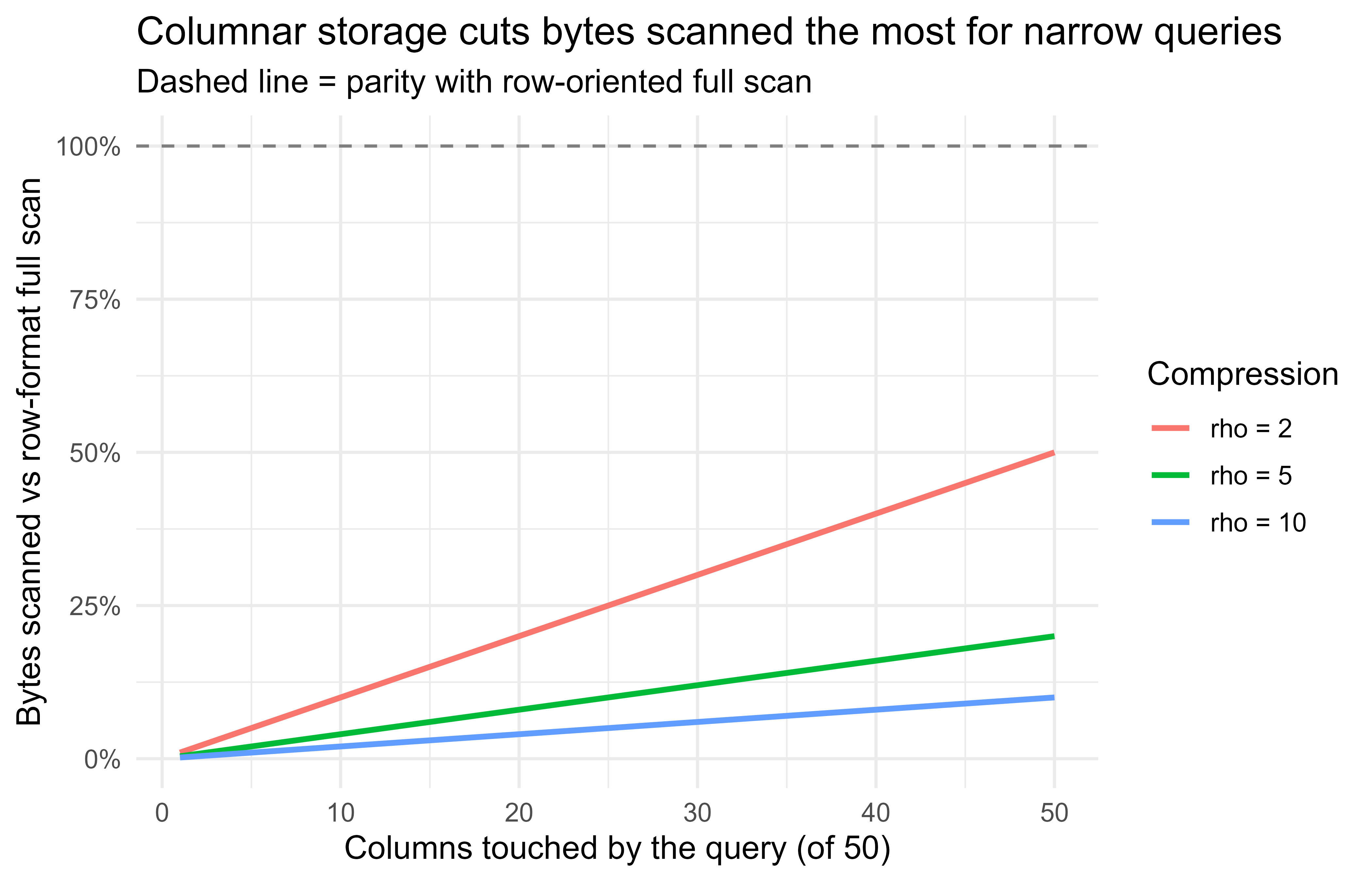
The cost equations earlier said bytes scanned and bytes transferred dominate analytics bills. Figure 105.1 makes the columnar-versus-row scanning model visible. We plot the bytes-scanned ratio from the formula \(\frac{1}{\rho}\cdot\frac{c}{p}\) as a function of how many columns a query touches, for a few compression factors \(\rho\).
Show code
p_cols<-50c_touched<-1:p_colsrho_vals<-c(2, 5, 10)df<-do.call(rbind, lapply(rho_vals, function(rho){data.frame( columns_touched =c_touched, ratio =(1/rho)*(c_touched/p_cols), rho =factor(paste0("rho = ", rho), levels =paste0("rho = ", rho_vals)))}))library(ggplot2)ggplot(df, aes(columns_touched, ratio, color =rho))+geom_hline(yintercept =1, linetype ="dashed", color ="grey50")+geom_line(linewidth =1)+scale_y_continuous(labels =scales::percent_format(accuracy =1))+labs( title ="Columnar storage cuts bytes scanned the most for narrow queries", subtitle ="Dashed line = parity with row-oriented full scan", x ="Columns touched by the query (of 50)", y ="Bytes scanned vs row-format full scan", color ="Compression")+theme_minimal(base_size =12)
Figure 105.1: Modeled bytes-scanned ratio (columnar vs row) as a query touches more of a 50-column table, for three compression factors. Lower is cheaper. Touching few columns in a well-compressed format is where the savings are largest.
The curves cross the parity line only when a query reads nearly every column and compression is weak. For the common case of touching a handful of columns in a compressed columnar file, the scanned-bytes ratio is a few percent, which is the practical reason lakehouse setups store Parquet rather than CSV.
105.8 Practical guidance, pitfalls, and when to use what
When to reach for each layer:
Use object storage as the durable home for raw data, intermediate datasets, and model artifacts. It is the cheapest place to keep bytes and the natural handoff point between pipeline stages.
Use a warehouse when you have structured data and analysts who write SQL or dplyr, and you want the engine to handle scale and concurrency.
Use a query engine over Parquet (arrow, duckdb) when you want warehouse-style queries without running a warehouse, especially for single-analyst or batch workloads (see Chapter 100).
Use remote compute only when the work genuinely exceeds one machine, and prefer scaling up before scaling out, because a single large instance avoids the overhead and serial fraction that Amdahl’s law penalizes.
Pitfalls that cost real money or break pipelines:
Egress surprises. Reading data across regions or out of the cloud is billed per gigabyte and is often the largest line on the bill. Keep compute in the storage region.
Pulling before reducing. collect() or get_object() on a huge table defeats the purpose of a warehouse. Inspect generated SQL with show_query() and confirm the reduction happens remotely.
Tiny-object storms. Millions of small objects make listing slow and run up per-request charges. Batch small records into larger Parquet files.
Hard-coded secrets. A key committed to git is compromised the moment it is pushed. Use attached identity or a secrets manager, and add credential files to .gitignore.
Pagination assumptions. list_objects_v2 returns at most 1000 keys per call. Loop on the continuation token or your listing silently truncates.
Forgetting idempotency. Network calls fail. Writes should be safe to retry (overwrite a deterministic key) so a retried job does not duplicate data.
Type drift on read. CSV loses column types; Parquet preserves them. If you must use CSV, pin column types explicitly on read rather than trusting inference.
A reasonable default architecture for a small team: land raw data as partitioned Parquet in one object-storage bucket in one region, query it with a serverless warehouse or DuckDB, keep model artifacts in the same bucket under a models/ prefix, and read credentials from attached identity in production and from .Renviron locally.
105.9 Further reading
Wickham, H., and Bryan, J. (2023). R Packages (2nd ed.). O’Reilly. Practical guidance on .Renviron, .gitignore, and keeping secrets out of code.
Wickham, H., Cetinkaya-Rundel, M., and Grolemund, G. (2023). R for Data Science (2nd ed.). O’Reilly. Covers DBI, dbplyr, and the lazy-then-collect() pattern for databases.
Kleppmann, M. (2017). Designing Data-Intensive Applications. O’Reilly. Storage engines, columnar formats, and the systems thinking behind warehouses.
Amdahl, G. M. (1967). Validity of the single processor approach to achieving large-scale computing capabilities. AFIPS Conference Proceedings.
Abadi, D., Boncz, P., and Harizopoulos, S. (2013). The Design and Implementation of Modern Column-Oriented Database Systems. Foundations and Trends in Databases. Why columnar scanning is cheap.
Luraschi, J., Kuo, K., and Ruiz, E. (2019). Mastering Spark with R. O’Reilly. The sparklyr model for distributed compute from R.
Not every warehouse bills this way. BigQuery’s on-demand mode bills bytes scanned, but provisioned systems like Redshift bill node-hours and Snowflake bills compute-seconds (credits). The bytes-scanned model is the cleanest one to reason about, and the design lessons below carry over: reading less data is always cheaper, whatever the meter.↩︎
Row-oriented means the file stores all the fields of record 1, then all the fields of record 2, and so on, so reading any column means stepping over the whole file. Columnar means the file stores all values of column 1 together, then all of column 2, so an engine can seek straight to the columns it needs and ignore the rest.↩︎
Swapping make_store() for a paws-backed store would mean reimplementing the five functions to call S3, with no change to any code that uses store$put, store$get, and friends. That is exactly the portability the real SDKs give you, and building the toy version is the fastest way to feel why.↩︎
Source Code
# Cloud Data and Compute from R {#sec-cloud-data-compute}```{r}#| include: falsesource("_common.R")```Most production data science no longer runs against a CSV on a laptop. The data lives in object storage, in a managed warehouse, or behind an API, and the compute that touches it runs on a rented machine somewhere else. This chapter is about how to reach that data and that compute from R, what the cost and performance trade-offs are, and how to write code that does not embed secrets or break when the dataset grows past memory.The focus is practical. The cloud chunks are marked `eval=FALSE` because this book builds without cloud credentials, but they are written to be correct and current so a reader with an account can run them. The one fully runnable demonstration is a small base-R abstraction that mirrors an object-store interface against a local directory, which teaches the mental model behind every cloud SDK.## Where this fits in a modern ML/AI workflowA typical workflow has three layers that used to live on one machine and now live in three different services:1. Storage: raw and processed data sits in object storage (Amazon S3, Google Cloud Storage, Azure Blob). Object storage is cheap, durable, and effectively unbounded, but it is a key-value store, not a filesystem, and not a query engine.2. Query and transform: structured analytics runs in a warehouse (BigQuery, Amazon Redshift, Snowflake) or a query engine over files (DuckDB, Spark). You push the computation to the data instead of pulling the data to R.3. Compute: model training and batch scoring run on rented CPU or GPU instances, sometimes orchestrated by a scheduler. R is often the client that submits the job and collects the result, not the thing doing the heavy lifting.The single most important habit is to move computation toward the data. Pulling a 200 GB table into R to compute a group mean wastes network, memory, and money. Issuing a `GROUP BY` to the warehouse and pulling back a few hundred rows is the same answer for a tiny fraction of the cost. The rest of this chapter is variations on that theme.::: {.callout-important title="Key idea"}Push the reduction to where the data lives, and transport only the small result back to R. Almost every recommendation in this chapter follows from that one sentence.:::### The cost model you are actually optimizingIt helps to write the total cost of a job as a sum of three terms:$$C_{\text{total}} = C_{\text{store}} + C_{\text{transfer}} + C_{\text{compute}}.$$Storage cost scales with bytes held over time,$$C_{\text{store}} = p_s \cdot B \cdot t,$$where $p_s$ is a per-gigabyte-month price, $B$ is bytes stored, and $t$ is months. Transfer cost is driven by data leaving a region or a cloud (egress),$$C_{\text{transfer}} = p_e \cdot B_{\text{out}} + p_r \cdot N_{\text{req}},$$with $p_e$ the egress price per gigabyte, $B_{\text{out}}$ the bytes read out, $p_r$ the per-request price, and $N_{\text{req}}$ the number of API calls. Compute cost for a warehouse query is often billed on bytes scanned,$$C_{\text{compute}} = p_q \cdot B_{\text{scan}},$$where $p_q$ is a per-terabyte-scanned price and $B_{\text{scan}}$ is bytes the engine read to answer the query.^[Not every warehouse bills this way. BigQuery's on-demand mode bills bytes scanned, but provisioned systems like Redshift bill node-hours and Snowflake bills compute-seconds (credits). The bytes-scanned model is the cleanest one to reason about, and the design lessons below carry over: reading less data is always cheaper, whatever the meter.] Two design choices fall straight out of these equations. First, columnar formats and partition pruning shrink $B_{\text{scan}}$, so they cut the dominant term for analytics. Second, keeping storage and compute in the same region drives $B_{\text{out}}$ toward zero, because in-region reads are usually free. A surprising fraction of real cloud bills is egress and request count, not storage.::: {.callout-warning}The term that surprises people on their first cloud bill is usually $C_{\text{transfer}}$, not $C_{\text{store}}$. Storing a terabyte for a month is cheap; reading it back across a region boundary or out to the public internet can cost more than storing it for a year. When a bill looks wrong, check egress first.:::## Object storage from RObject storage exposes a flat namespace: a bucket holds objects, each addressed by a key (a string that may contain slashes so it looks like a path). There are no real directories. Listing "a folder" is really listing all keys with a common prefix. The core operations are small: put an object, get an object, list keys under a prefix, delete an object, and check existence.::: {.callout-tip title="Intuition"}Think of a bucket as one giant hash map from string keys to blobs of bytes, not as a tree of folders. The slashes in `datasets/2025/events.parquet` are just characters in the key. The console draws them as folders for your comfort, but the storage layer never moves up or down a directory because there is no directory to move through.:::The main R interfaces are `paws` (a generated AWS SDK covering S3 and much else), `googleCloudStorageR` for GCS, and `AzureStor` for Azure Blob. Below is idiomatic `paws` code for the five core operations. It will not run here because there are no credentials, but it is the shape you will use.```{r s3-paws, eval=FALSE}library(paws)# Credentials are read from the standard chain: environment variables,# ~/.aws/credentials, or an instance/role profile. Never hard-code keys.s3 <- paws::s3()bucket <-"my-ml-bucket"# PUT: upload a serialized R objectsaveRDS(mtcars, "mtcars.rds")s3$put_object(Bucket = bucket,Key ="datasets/mtcars.rds",Body =readBin("mtcars.rds", "raw", n =file.size("mtcars.rds")))# LIST: enumerate keys under a prefix (note: paginated, max 1000 per call)listing <- s3$list_objects_v2(Bucket = bucket, Prefix ="datasets/")vapply(listing$Contents, function(o) o$Key, character(1))# EXISTS: a head request is cheap and avoids downloading the bodyexists_obj <-tryCatch({ s3$head_object(Bucket = bucket, Key ="datasets/mtcars.rds")TRUE}, error =function(e) FALSE)# GET: download to a raw vector, then deserializeobj <- s3$get_object(Bucket = bucket, Key ="datasets/mtcars.rds")tmp <-tempfile(fileext =".rds")writeBin(obj$Body, tmp)restored <-readRDS(tmp)# DELETEs3$delete_object(Bucket = bucket, Key ="datasets/mtcars.rds")```The equivalent in `googleCloudStorageR` is higher level because it has explicit upload and download helpers:```{r gcs, eval=FALSE}library(googleCloudStorageR)# Auth via a service-account JSON key referenced by an env var, not a literal path in code.gcs_auth(json_file =Sys.getenv("GCS_AUTH_FILE"))gcs_global_bucket("my-ml-bucket")gcs_upload(mtcars, name ="datasets/mtcars.rds") # PUTobjs <-gcs_list_objects(prefix ="datasets/") # LISTrestored <-gcs_get_object("datasets/mtcars.rds", # GETsaveToDisk =tempfile(),overwrite =TRUE)gcs_delete_object("datasets/mtcars.rds") # DELETE```And Azure Blob through `AzureStor`:```{r azure, eval=FALSE}library(AzureStor)endp <-storage_endpoint("https://myaccount.blob.core.windows.net",key =Sys.getenv("AZURE_STORAGE_KEY"))cont <-storage_container(endp, "my-ml-container")storage_upload(cont, src ="mtcars.rds", dest ="datasets/mtcars.rds") # PUTlist_storage_files(cont, dir ="datasets") # LISTstorage_download(cont, src ="datasets/mtcars.rds", dest =tempfile()) # GETdelete_storage_file(cont, "datasets/mtcars.rds") # DELETE```Across all three providers the interface is the same five verbs over a key-value store. Once you internalize that, switching clouds is mostly renaming functions.::: {.callout-note}The body of an S3 object comes back as a raw byte vector, which is why the `paws` example writes it to a temporary file before `readRDS()`. The higher-level GCS and Azure helpers hide that step behind a `saveToDisk`/`dest` argument, but underneath they are doing the same thing.:::### File formats matter more than the SDKWhat you store under those keys decides your query cost. The choice is usually between a row-oriented text format (CSV) and a columnar binary format (Parquet); the formats themselves are treated more fully in @sec-data-formats.^[Row-oriented means the file stores all the fields of record 1, then all the fields of record 2, and so on, so reading any column means stepping over the whole file. Columnar means the file stores all values of column 1 together, then all of column 2, so an engine can seek straight to the columns it needs and ignore the rest.] Columnar storage lets an engine read only the columns a query touches, and it compresses far better because values within a column share a type and a distribution.A back-of-the-envelope model: if a query needs $c$ of $p$ columns and the columnar format compresses by factor $\rho$, the bytes scanned drop roughly by$$\frac{B_{\text{scan}}^{\text{columnar}}}{B_{\text{scan}}^{\text{row}}} \approx \frac{1}{\rho}\cdot\frac{c}{p}.$$For a wide table where a query touches a few columns, this is often a 10x to 100x reduction, which maps directly onto the $C_{\text{compute}} = p_q \cdot B_{\text{scan}}$ term above. In R you would write Parquet with `arrow`:```{r arrow-parquet, eval=FALSE}library(arrow)# Write a partitioned Parquet dataset directly to S3.# Partitioning by a frequently filtered column lets the reader skip whole files.arrow::write_dataset(dataset = my_data_frame,path ="s3://my-ml-bucket/datasets/events/",format ="parquet",partitioning =c("year", "month"))# Read back lazily: filters and column selection are pushed down,# so only the needed partitions and columns are fetched.ds <- arrow::open_dataset("s3://my-ml-bucket/datasets/events/")library(dplyr)result <- ds |>filter(year ==2025, month ==6) |>select(user_id, amount) |>group_by(user_id) |>summarise(total =sum(amount)) |>collect() # only this line pulls data into R```## Cloud databases and warehouses from RA warehouse is a managed SQL engine that separates storage from compute and scales the compute elastically. From R, the standard route is the `DBI` interface plus a driver package, so the same R code talks to BigQuery, Redshift, Snowflake, or a local SQLite by swapping the connection object.::: {.callout-tip title="Intuition"}`DBI` is to databases what a wall socket is to appliances. Your R code (the appliance) plugs into a standard interface; the driver package (the plug) handles whatever the specific warehouse expects behind the wall. Change the warehouse and you change the plug, not the appliance.:::```{r dbi-bq, eval=FALSE}library(DBI)library(bigrquery) # BigQuery driver implementing the DBI genericcon <-dbConnect( bigrquery::bigquery(),project =Sys.getenv("GCP_PROJECT"),dataset ="analytics")# Push the aggregation to the warehouse; pull back only the summary.res <-dbGetQuery(con, " SELECT user_id, SUM(amount) AS total FROM analytics.events WHERE event_date >= '2025-01-01' GROUP BY user_id")dbDisconnect(con)```The same pattern with Redshift or Snowflake just changes the driver:```{r dbi-others, eval=FALSE}library(DBI)# Redshift speaks the PostgreSQL wire protocol, so RPostgres works.con_rs <-dbConnect( RPostgres::Redshift(),host =Sys.getenv("REDSHIFT_HOST"),port =5439,dbname ="warehouse",user =Sys.getenv("REDSHIFT_USER"),password =Sys.getenv("REDSHIFT_PASSWORD"))# Snowflake via the odbc package and the Snowflake ODBC driver.con_sf <-dbConnect( odbc::odbc(),Driver ="SnowflakeDSIIDriver",Server =Sys.getenv("SNOWFLAKE_ACCOUNT"),UID =Sys.getenv("SNOWFLAKE_USER"),PWD =Sys.getenv("SNOWFLAKE_PASSWORD"),Warehouse ="COMPUTE_WH",Database ="ANALYTICS")```The most useful pattern for analysts is to let `dbplyr` translate `dplyr` verbs into SQL so you never hand-write the query, and so the computation stays in the warehouse until you call `collect()`:```{r dbplyr, eval=FALSE}library(dplyr)library(dbplyr)events <-tbl(con, "events") # a lazy reference, no data moved yetsummary_tbl <- events |>filter(event_date >="2025-01-01") |>group_by(user_id) |>summarise(total =sum(amount), n =n())show_query(summary_tbl) # inspect the generated SQLlocal_result <-collect(summary_tbl) # execute remotely, fetch the small result```The discipline is identical to object storage: do the reduction remotely, transport the small thing.::: {.callout-tip}The lazy reference `events` looks like a data frame but holds no rows. Nothing runs until `collect()`. Get in the habit of calling `show_query()` before `collect()` so you can confirm the filter and the `GROUP BY` were pushed to the warehouse, not quietly applied in R after a full download.:::## Comparison of the main options@tbl-cloud-data-compute-options summarizes the storage and query options discussed, with the R package you would reach for and the cost driver to watch. Prices change constantly, so the table gives the billing model, not numbers.| Service | Type | Primary R interface | Billing driver | Best for ||---|---|---|---|---|| Amazon S3 | Object storage |`paws`| Storage GB-month, requests, egress | Raw data lake, model artifacts || Google Cloud Storage | Object storage |`googleCloudStorageR`| Storage GB-month, operations, egress | Same, GCP-native pipelines || Azure Blob | Object storage |`AzureStor`| Storage GB-month, operations, egress | Same, Azure-native pipelines || BigQuery | Serverless warehouse |`bigrquery` + `DBI`| Bytes scanned per query | Ad hoc analytics, no cluster to manage || Amazon Redshift | Provisioned warehouse |`RPostgres` + `DBI`| Cluster node-hours | Steady heavy workloads on AWS || Snowflake | Elastic warehouse |`odbc` + `DBI`| Warehouse credits (compute-seconds) | Bursty multi-team analytics || Parquet on object store | File + query engine |`arrow`, `duckdb`| Bytes scanned (engine) + storage | Cheap columnar lakehouse queries |: Storage and query options for cloud data work from R, with the primary R interface, the billing driver to watch, and the workload each option suits best. {#tbl-cloud-data-compute-options}A rough rule: object storage is where bytes rest, a warehouse or query engine is where bytes are reduced, and the choice among warehouses is mostly about whether your load is steady (provisioned) or bursty (serverless or elastic).## Credentials and secretsA credential, an access key or password that proves you may read a bucket or query a warehouse, is the most dangerous thing in a data pipeline, because a leaked one gives a stranger your access and your bill. The cardinal rule is that secrets never appear in source code, in notebooks, or in version control. The mechanisms, in rough order of preference:1. Identity attached to the compute (an IAM role on an EC2 instance, a workload identity on a GCP VM, a managed identity on Azure). The SDK picks up short-lived credentials automatically and there is nothing to leak.2. A secrets manager (AWS Secrets Manager, GCP Secret Manager, Azure Key Vault, or HashiCorp Vault) that the application reads at run time.3. Environment variables set by the deployment, read in R with `Sys.getenv()`.4. A local config file outside the repo, such as `~/.aws/credentials` or a service-account JSON, referenced by path through an env var.In R, `Sys.getenv("NAME")` returns `""` for an unset variable, so guard against silent misconfiguration:```{r creds-guard, eval=FALSE}get_required_env <-function(name) { val <-Sys.getenv(name, unset =NA_character_)if (is.na(val) ||!nzchar(val)) {stop(sprintf("Required environment variable %s is not set", name),call. =FALSE) } val}aws_key <-get_required_env("AWS_ACCESS_KEY_ID")```For local development, the `.Renviron` file holds variables outside the script, and the `keyring` package stores secrets in the operating system credential store. Whatever you do, add credential files to `.gitignore` and prefer attached identity in production so there is no long-lived key to rotate or lose.::: {.callout-warning}A secret committed to git is compromised the moment the commit is pushed, and deleting it later does not help because it lives forever in the repository history. Treat any key that touches version control as already leaked: rotate it immediately rather than hoping nobody noticed.:::## Remote computeSo far the data was too big for the laptop but the computation was light. Sometimes the reverse is true: the dataset fits, but training the model is what overwhelms one machine. When the model, not just the data, is too big for the laptop, the compute moves too. The common patterns from R:- Submit a job to a managed batch service or a cluster scheduler and poll for completion. R is the client.- Use a distributed engine such as Spark through `sparklyr`, which translates `dplyr` and MLlib calls into work on the cluster (covered in depth in @sec-spark-sparklyr).- Train on a remote GPU instance with `keras`/`tensorflow` or `torch`, where R drives the training loop on hardware you rented (see @sec-torch-for-r).A `sparklyr` sketch, where the data and the model fit both stay on the cluster:```{r sparklyr, eval=FALSE}library(sparklyr)library(dplyr)sc <-spark_connect(master ="yarn") # or a Databricks/standalone masterevents <-spark_read_parquet(sc, "events", "s3a://my-ml-bucket/datasets/events/")model <- events |>filter(!is.na(amount)) |>ml_linear_regression(amount ~ feature_1 + feature_2)summary(model)spark_disconnect(sc)```A GPU training sketch with `keras`, kept `eval=FALSE` because it needs a configured backend:```{r keras-remote, eval=FALSE}library(keras)model <-keras_model_sequential() |>layer_dense(units =128, activation ="relu", input_shape =ncol(x_train)) |>layer_dropout(0.3) |>layer_dense(units =1)model |>compile(optimizer ="adam", loss ="mse")model |>fit(x_train, y_train, epochs =20, batch_size =256,validation_split =0.2)```The decision of whether to scale up (a bigger single machine) or scale out (many machines) is governed by how the work parallelizes. If a job splits into $n$ independent tasks of which a fraction $s$ must run serially, Amdahl's law bounds the speedup from $k$ workers at$$\text{speedup}(k) = \frac{1}{s + \frac{1-s}{k}},$$which approaches $1/s$ as $k \to \infty$. The practical reading: distributing only pays when the serial fraction $s$ is small and the per-task overhead is much smaller than the per-task work. Many "embarrassingly parallel" jobs (scoring rows, fitting independent models per group) have $s$ near zero and scale almost linearly; iterative algorithms with a synchronization barrier each step do not.::: {.callout-tip title="When to use this"}Reach for a distributed engine like Spark only after a single large instance is genuinely too small. A 64-core machine with a few hundred gigabytes of RAM handles a lot, and it has no network shuffle, no cluster to babysit, and no serial-fraction penalty. Scale up first; scale out when up runs out.:::## A runnable demo: a local store that mirrors an object-store interfaceThe cleanest way to understand cloud SDKs is to build the abstraction yourself against a local directory. The five verbs (put, get, list, exists, delete) and the flat key namespace are exactly what S3, GCS, and Blob expose. The function factory below returns a small "store" backed by a temp directory, keys are arbitrary strings, and objects are R values serialized to disk. Code that uses this store would not change if you swapped the backend for `paws`.```{r local-store, eval=TRUE}# A function factory returning an object-store-like interface over a local dir.# Keys are strings (slashes allowed but treated as literal characters, not paths).make_store <-function(root =tempfile("store_")) {dir.create(root, showWarnings =FALSE, recursive =TRUE)# Encode an arbitrary key to a safe single filename so "a/b" is one object,# not a nested directory. This mirrors object storage's flat namespace. key_to_path <-function(key) { safe <-gsub("([^A-Za-z0-9_.-])", "_", key)file.path(root, paste0(safe, ".rds")) }# Keep a sidecar index mapping safe filenames back to original keys. index_file <-file.path(root, ".keys.rds") read_index <-function() if (file.exists(index_file)) readRDS(index_file) elsecharacter(0) write_index <-function(ix) saveRDS(ix, index_file)list(put =function(key, value) {saveRDS(value, key_to_path(key)) ix <-read_index() ix[basename(key_to_path(key))] <- keywrite_index(ix)invisible(key) },get =function(key) { p <-key_to_path(key)if (!file.exists(p)) stop(sprintf("NoSuchKey: %s", key), call. =FALSE)readRDS(p) },exists =function(key) file.exists(key_to_path(key)),delete =function(key) { p <-key_to_path(key)if (file.exists(p)) file.remove(p) ix <-read_index(); ix <- ix[names(ix) !=basename(p)]; write_index(ix)invisible(NULL) },list_keys =function(prefix ="") { ix <-read_index() keys <-unname(ix) keys[startsWith(keys, prefix)] } )}# Exercise the interface exactly as you would a cloud store.store <-make_store()store$put("datasets/mtcars", mtcars)store$put("datasets/iris", iris)store$put("models/lm_mpg", lm(mpg ~ wt + hp, data = mtcars))cat("Keys under 'datasets/':\n")print(store$list_keys(prefix ="datasets/"))cat("\nExists 'models/lm_mpg':", store$exists("models/lm_mpg"), "\n")cat("Exists 'models/missing':", store$exists("models/missing"), "\n")restored <- store$get("datasets/mtcars")cat("\nRound-trip identical to original mtcars:",identical(restored, mtcars), "\n")```The point is that the consuming code is provider-agnostic.^[Swapping `make_store()` for a `paws`-backed store would mean reimplementing the five functions to call S3, with no change to any code that uses `store$put`, `store$get`, and friends. That is exactly the portability the real SDKs give you, and building the toy version is the fastest way to feel why.] Now we use the demo to make the cost argument concrete: pushing a reduction to the store versus pulling everything back, the same trade-off as the $C_{\text{transfer}}$ term at the start of the chapter.```{r push-vs-pull, eval=TRUE}# Simulate "remote reduction" vs "pull everything then reduce" in terms of# bytes transported back to the client. The store can compute a summary in place.# Add a server-side aggregate to a store: it reads the object on the "server"# and returns only the small result, mimicking a warehouse GROUP BY.store$aggregate <-function(key, fun) fun(store$get(key))# Put a moderately large frame in the store.set.seed(1)big <-data.frame(grp =sample(letters[1:5], 2e5, replace =TRUE),x =rnorm(2e5))store$put("datasets/big", big)bytes_of <-function(obj) length(serialize(obj, connection =NULL))# Strategy A: pull the whole object to the client, then reduce locally.pulled <- store$get("datasets/big")client_summary <-aggregate(x ~ grp, data = pulled, FUN = mean)bytes_pulled <-bytes_of(pulled)# Strategy B: reduce on the "server", transport only the summary.server_summary <- store$aggregate("datasets/big",function(d) aggregate(x ~ grp, d, mean))bytes_summary <-bytes_of(server_summary)cat(sprintf("Pull-everything transported : %s bytes\n",format(bytes_pulled, big.mark =",")))cat(sprintf("Remote-reduce transported : %s bytes\n",format(bytes_summary, big.mark =",")))cat(sprintf("Reduction factor : %.0fx\n", bytes_pulled / bytes_summary))# Both strategies give the same answer.cat("Same result:", isTRUE(all.equal(client_summary, server_summary,check.attributes =FALSE)), "\n")```Both strategies return the identical group means, but the remote reduction moves a few hundred bytes instead of a few megabytes, a reduction of four orders of magnitude on this small frame and far more on a real one. That ratio is the entire economic argument for warehouses and pushdown queries, made visible in base R.### A figure: where the cost goesThe cost equations earlier said bytes scanned and bytes transferred dominate analytics bills. @fig-cloud-data-compute-scan-ratio makes the columnar-versus-row scanning model visible. We plot the bytes-scanned ratio from the formula $\frac{1}{\rho}\cdot\frac{c}{p}$ as a function of how many columns a query touches, for a few compression factors $\rho$.```{r fig-cloud-data-compute-scan-ratio, eval=TRUE, fig.width=7, fig.height=4.5, fig.cap="Modeled bytes-scanned ratio (columnar vs row) as a query touches more of a 50-column table, for three compression factors. Lower is cheaper. Touching few columns in a well-compressed format is where the savings are largest."}p_cols <-50c_touched <-1:p_colsrho_vals <-c(2, 5, 10)df <-do.call(rbind, lapply(rho_vals, function(rho) {data.frame(columns_touched = c_touched,ratio = (1/ rho) * (c_touched / p_cols),rho =factor(paste0("rho = ", rho), levels =paste0("rho = ", rho_vals)) )}))library(ggplot2)ggplot(df, aes(columns_touched, ratio, color = rho)) +geom_hline(yintercept =1, linetype ="dashed", color ="grey50") +geom_line(linewidth =1) +scale_y_continuous(labels = scales::percent_format(accuracy =1)) +labs(title ="Columnar storage cuts bytes scanned the most for narrow queries",subtitle ="Dashed line = parity with row-oriented full scan",x ="Columns touched by the query (of 50)",y ="Bytes scanned vs row-format full scan",color ="Compression" ) +theme_minimal(base_size =12)```The curves cross the parity line only when a query reads nearly every column and compression is weak. For the common case of touching a handful of columns in a compressed columnar file, the scanned-bytes ratio is a few percent, which is the practical reason lakehouse setups store Parquet rather than CSV.## Practical guidance, pitfalls, and when to use whatWhen to reach for each layer:- Use object storage as the durable home for raw data, intermediate datasets, and model artifacts. It is the cheapest place to keep bytes and the natural handoff point between pipeline stages.- Use a warehouse when you have structured data and analysts who write SQL or `dplyr`, and you want the engine to handle scale and concurrency.- Use a query engine over Parquet (`arrow`, `duckdb`) when you want warehouse-style queries without running a warehouse, especially for single-analyst or batch workloads (see @sec-duckdb-arrow).- Use remote compute only when the work genuinely exceeds one machine, and prefer scaling up before scaling out, because a single large instance avoids the overhead and serial fraction that Amdahl's law penalizes.Pitfalls that cost real money or break pipelines:- Egress surprises. Reading data across regions or out of the cloud is billed per gigabyte and is often the largest line on the bill. Keep compute in the storage region.- Pulling before reducing. `collect()` or `get_object()` on a huge table defeats the purpose of a warehouse. Inspect generated SQL with `show_query()` and confirm the reduction happens remotely.- Tiny-object storms. Millions of small objects make listing slow and run up per-request charges. Batch small records into larger Parquet files.- Hard-coded secrets. A key committed to git is compromised the moment it is pushed. Use attached identity or a secrets manager, and add credential files to `.gitignore`.- Pagination assumptions. `list_objects_v2` returns at most 1000 keys per call. Loop on the continuation token or your listing silently truncates.- Forgetting idempotency. Network calls fail. Writes should be safe to retry (overwrite a deterministic key) so a retried job does not duplicate data.- Type drift on read. CSV loses column types; Parquet preserves them. If you must use CSV, pin column types explicitly on read rather than trusting inference.A reasonable default architecture for a small team: land raw data as partitioned Parquet in one object-storage bucket in one region, query it with a serverless warehouse or DuckDB, keep model artifacts in the same bucket under a `models/` prefix, and read credentials from attached identity in production and from `.Renviron` locally.## Further reading- Wickham, H., and Bryan, J. (2023). *R Packages* (2nd ed.). O'Reilly. Practical guidance on `.Renviron`, `.gitignore`, and keeping secrets out of code.- Wickham, H., Cetinkaya-Rundel, M., and Grolemund, G. (2023). *R for Data Science* (2nd ed.). O'Reilly. Covers `DBI`, `dbplyr`, and the lazy-then-`collect()` pattern for databases.- Kleppmann, M. (2017). *Designing Data-Intensive Applications*. O'Reilly. Storage engines, columnar formats, and the systems thinking behind warehouses.- Amdahl, G. M. (1967). Validity of the single processor approach to achieving large-scale computing capabilities. *AFIPS Conference Proceedings*.- Abadi, D., Boncz, P., and Harizopoulos, S. (2013). *The Design and Implementation of Modern Column-Oriented Database Systems*. Foundations and Trends in Databases. Why columnar scanning is cheap.- Luraschi, J., Kuo, K., and Ruiz, E. (2019). *Mastering Spark with R*. O'Reilly. The `sparklyr` model for distributed compute from R.