Advanced Data Analysis

Nguyen, Mike

10 Bagging

A single decision tree, like CART (see the classification and regression trees chapter, Chapter 8) or MARS (Chapter 9), is easy to read but unstable. If you split your training data into two halves at random and grow a tree on each half, you can end up with two very different trees that make very different predictions. This sensitivity to the particular sample you happened to draw is what statisticians call high variance, and it is the main reason a lone tree often predicts poorly on new data.

This chapter introduces a remedy called bagging, short for bootstrap aggregation. The idea is simple and powerful: instead of trusting one unstable tree, grow many trees on slightly different versions of the data and average their predictions. Averaging cancels out the random wobble of any individual tree, so the combined predictor is far more stable than its parts. By the end of the chapter you will understand why averaging reduces variance, how the bootstrap lets us mimic having many training sets when we really have only one, how to estimate test error for free using out-of-bag samples, and how to measure variable importance once the trees are no longer individually interpretable. Bagging is also the conceptual stepping stone to random forests (Chapter 13), which we preview here.

Intuition

Think of each tree as a noisy measurement of the same underlying quantity. One measurement is unreliable, but the average of many independent measurements is close to the truth. Bagging applies that everyday logic to prediction models.

10.1 Why averaging reduces variance

Some procedures are naturally stable. Ordinary linear regression, for example, gives nearly the same fit whether you run it on one random sample or another, especially when the number of observations $n$ is large relative to the number of predictors $p$. A procedure with low variance yields similar results when applied repeatedly to distinct data sets. Trees are the opposite: they are flexible enough to chase noise, so small changes in the data produce large changes in the fitted model.

Bagging is a general-purpose procedure for reducing the variance of any such unstable method.¹ The strategy is to average many models. If we had access to $B$ separate training sets, we could fit a model on each, call them $\hat{f}^1(X), \hat{f}^2(X), \dots, \hat{f}^B(X)$, and average them into a single bagged predictor:

\[ \hat{f}_{bag} (X) = \frac{1}{B} \sum_{b=1}^B \hat{f}^b (x) \]

Key idea

Averaging keeps the bias of the base model roughly the same while shrinking its variance. That is why we deliberately grow each tree large and unpruned: large trees have low bias but high variance, and averaging takes care of the variance.

10.1.1 The variance-reduction identity

Fix a test point $x$ and treat each base prediction $\hat f^b(x)$ as a random variable, with the randomness coming from the training sample (and, for bootstrap bagging, from the resampling). Suppose the $B$ predictors are identically distributed, each with mean $\mu(x) = \mathbb{E}[\hat f^b(x)]$ and variance $\sigma^2(x) = \operatorname{Var}(\hat f^b(x))$, and with a common pairwise correlation \[ \rho(x) \;=\; \operatorname{Corr}\!\big(\hat f^b(x),\,\hat f^{b'}(x)\big), \qquad b \neq b'. \] The bagged predictor is the average $\hat f_{bag}(x) = \tfrac{1}{B}\sum_b \hat f^b(x)$. Its mean is unchanged, $\mathbb{E}[\hat f_{bag}(x)] = \mu(x)$, so bagging does not alter bias under this model. For the variance, expand the variance of a sum: \[ \operatorname{Var}\!\Big(\tfrac{1}{B}\textstyle\sum_{b=1}^B \hat f^b(x)\Big) = \frac{1}{B^2}\Big[\sum_{b=1}^B \operatorname{Var}(\hat f^b) + \sum_{b\neq b'}\operatorname{Cov}(\hat f^b,\hat f^{b'})\Big]. \] There are $B$ variance terms each equal to $\sigma^2$, and $B(B-1)$ covariance terms each equal to $\rho\sigma^2$. Substituting, \[ \operatorname{Var}(\hat f_{bag}(x)) = \frac{1}{B^2}\big[B\sigma^2 + B(B-1)\rho\sigma^2\big] = \rho\,\sigma^2 + \frac{1-\rho}{B}\,\sigma^2 . \tag{10.1}\]

Equation 10.1 is the central theoretical fact about bagging. Read it term by term:

As $B \to \infty$ the second term vanishes, leaving the floor $\rho\sigma^2$. You cannot average away the part of the variance that the trees share. This is exactly why decorrelating the trees, by sampling a subset of $m < p$ predictors at each split, lowers the floor and motivates random forests (Chapter 13).
If the predictors were independent ($\rho = 0$) the variance would collapse to $\sigma^2/B$, the classical $1/B$ rate for averaging i.i.d. quantities. Bootstrap samples overlap heavily, so in practice $\rho$ is well above zero and most of the gain is realized within the first one to two hundred trees.

Note

The decomposition assumes a common correlation $\rho \ge 0$, which holds for bootstrap-trained trees because they share the same underlying data. Adding trees can only reduce $\operatorname{Var}(\hat f_{bag})$ toward the floor $\rho\sigma^2$; it never increases it. This is the precise sense in which “more trees never overfit” in bagging: $B$ is a smoothing parameter for the Monte Carlo average, not a model-complexity knob.

10.1.2 Why bagging helps unstable learners and can hurt stable ones

Variance reduction is not a free lunch for every base learner. Consider the idealized aggregated predictor that averages over the true sampling distribution of the data, $f_{A}(x) = \mathbb{E}_{\mathcal D}[\hat f(x;\mathcal D)]$, where $\mathcal D$ is a training set of size $n$. For squared-error loss with a fixed target $y$, expand around $f_A$: \[ \mathbb{E}_{\mathcal D}\big[(y - \hat f(x;\mathcal D))^2\big] = (y - f_A(x))^2 + \mathbb{E}_{\mathcal D}\big[(\hat f(x;\mathcal D) - f_A(x))^2\big] \ge (y - f_A(x))^2 . \tag{10.2}\]

The cross term cancels because $\mathbb{E}_{\mathcal D}[\hat f - f_A] = 0$, and the remaining term is the variance of the base learner. Equation 10.2 says the aggregated predictor’s squared error never exceeds the average squared error of the base learner, and the gap is precisely the variance. The more variable (unstable) the learner, the larger the improvement; for a perfectly stable learner the gap is zero and bagging does nothing. Bagging approximates $f_A$ by the bootstrap average, so it inherits this behavior: large gains for high-variance learners like deep trees, negligible or even slightly negative effects for low-variance learners like linear regression, because the bootstrap approximation introduces its own small error.

Warning

For classification the squared-error argument does not transfer directly, and voting can in rare cases make a good classifier worse. If the base classifier is already better than random in a region, majority voting pushes its accuracy toward $1$ there; but in regions where it is worse than random, voting amplifies the error toward $0$. Bagging therefore helps “order-correct” classifiers and can degrade poor ones. In practice with reasonable trees this almost never bites, but it explains why bagging is not universally beneficial.

10.2 The bootstrap: many data sets from one

There is a practical problem with the recipe above. In reality we almost never have $B$ independent training sets; we have a single sample. The bootstrap solves this by manufacturing surrogate data sets from the one we have. To create a bootstrap sample, we draw observations from the original training set at random with replacement until we have a data set of the same size. Because we sample with replacement, some observations appear more than once and others not at all, so each bootstrap sample differs slightly from the original.

We generate $B$ such bootstrap samples, fit a model on each, and average the fits. The bagged prediction $\hat{f}_{bag}(x)$ is the average of the fits from these $B$ bootstrap samples, exactly as in the formula above but with bootstrap samples standing in for genuine independent training sets.

10.2.1 How much of the data does a bootstrap sample see?

The “roughly one third left out” figure quoted below is not a rule of thumb but an exact limit. A bootstrap sample is drawn by taking $n$ independent draws, each uniform over the $n$ training indices. The probability that a particular observation $i$ is missed on a single draw is $1 - \tfrac{1}{n}$, and since the draws are independent the probability it is missed on all $n$ draws is \[ \Pr(i \notin \text{bootstrap sample}) = \Big(1 - \frac{1}{n}\Big)^{n}. \tag{10.3}\]

Using $\big(1 - \tfrac{1}{n}\big)^{n} = \exp\!\big[n\ln(1 - \tfrac1n)\big]$ and the expansion $\ln(1 - \tfrac1n) = -\tfrac1n - \tfrac{1}{2n^2} - \cdots$, the exponent tends to $-1$, so \[ \lim_{n\to\infty}\Big(1 - \frac{1}{n}\Big)^{n} = e^{-1} \approx 0.368 . \] About $36.8\%$ of observations are out-of-bag for any given tree, and the complementary $\approx 63.2\%$ are in-bag (the distinct observations appearing at least once; of these, about $36.8\%$ of all observations appear exactly once and about $26.4\%$ appear more than once). The convergence is fast: even at $n = 20$ the omission probability is $0.358$. This single number underlies both the out-of-bag error estimate below and the effective training-set size each tree sees.

Note

With regression trees, we construct $B$ trees and average their predictions, growing each tree large with no pruning. Each tree on its own has high variance and low bias; averaging then drives the variance down without inflating the bias. In practice, around 100 trees is usually enough to capture most of the variance reduction.

For classification the averaging step changes slightly because we cannot average class labels directly. Instead, we record the class predicted by each of the $B$ trees for a given test observation and take a majority vote, choosing the category that occurs most often across the trees.

10.3 Out-of-bag error: cross-validation for free

A pleasant side effect of the bootstrap is that we can estimate test error without performing cross-validation. The reason is that each bootstrap sample leaves some observations out by construction.

The procedure works as follows. For a given tree, the observations that were not selected into its bootstrap sample are called the out-of-bag (OOB) observations for that tree.² To get an OOB prediction for the $i$-th observation, we use only the trees in which that observation was OOB, and average their predictions. Comparing these OOB predictions against the true responses gives the OOB MSE for regression, or the OOB classification error for classification.

Formally, let $O_i = \{\, b : i \notin \text{bootstrap sample } b \,\}$ be the set of trees for which observation $i$ is out-of-bag. The OOB prediction and the OOB error estimate are \[ \hat f^{\,\text{oob}}(x_i) = \frac{1}{|O_i|}\sum_{b \in O_i} \hat f^b(x_i), \qquad \widehat{\text{Err}}_{\text{oob}} = \frac{1}{n}\sum_{i=1}^n L\big(y_i,\, \hat f^{\,\text{oob}}(x_i)\big), \tag{10.4}\] with $L$ the squared error for regression or the $0/1$ loss (via the OOB majority vote) for classification. Because each $\hat f^{\,\text{oob}}(x_i)$ averages over only $|O_i| \approx 0.368\,B$ trees, the OOB estimate for a forest of $B$ trees behaves like a test estimate for a smaller forest of about $0.368\,B$ trees; it is therefore mildly pessimistic when $B$ is small, and the bias disappears as $B$ grows. The OOB estimate is nearly equivalent to leave-one-out cross-validation but costs nothing extra, since the trees are already fit. Its main limitation is that the $\hat f^{\,\text{oob}}(x_i)$ are not independent across $i$ (they share trees), so the OOB error has no simple standard error.

Key idea

The OOB error is a valid estimate of the test error because each observation is predicted only by trees that never saw it during training. No data point judges a model that was trained on it.

We can confirm the omission probability of Equation 10.3 and the resulting OOB share by direct simulation.

Show code

set.seed(1)
n <- 200
B <- 2000
in_bag <- replicate(B, sort(unique(sample(1:n, n, replace = TRUE))))
oob_fraction <- mean(sapply(in_bag, function(s) (n - length(s)) / n))
c(simulated = oob_fraction, theoretical = (1 - 1/n)^n, limit = exp(-1))
#>   simulated theoretical       limit 
#>   0.3664225   0.3669578   0.3678794

The simulated out-of-bag fraction matches $(1 - 1/n)^n$ and its limit $e^{-1}$.

10.4 The cost: losing interpretability

Bagging buys predictive accuracy, but it gives up the clarity that made a single tree appealing. A lone tree can be drawn as a flowchart and read top to bottom. Once we average over hundreds of trees, the variable used at each split (or the basis function included) can change dramatically from tree to tree, so there is no single diagram to interpret and no obvious way to say which variable matters most.

To recover some interpretation, we track how much each predictor contributes to the trees, averaged over all $B$ of them. The two standard measures of variable importance are:

For regression, the total amount by which the residual sum of squares is decreased due to splits on a given predictor, averaged over all $B$ trees.
For classification, the total amount by which the Gini index is decreased by splits on a given predictor, averaged over all $B$ trees.

A predictor that consistently produces large reductions in error across the ensemble is judged important, even though we can no longer point to a single tree to explain why. Variable importance is one of several tools for understanding otherwise opaque models, a topic taken up more broadly in the interpretable machine learning chapter (Chapter 35).

10.4.1 Two importance measures, made precise

The randomForest output reports two distinct quantities, and it is worth stating each exactly because they can disagree.

Impurity (Gini / RSS) importance. When a split on variable $j$ at node $t$ in tree $b$ reduces node impurity by $\Delta i_t$ (the drop in RSS for regression, or in the Gini index $G_t = \sum_k \hat p_{tk}(1 - \hat p_{tk})$ for classification), accumulate that decrease. The importance of $X_j$ is the total over all nodes that split on $j$, averaged over trees: \[ \text{Imp}^{\text{imp}}(X_j) = \frac{1}{B}\sum_{b=1}^B \;\sum_{t \in T_b\,:\, v(t)=j} \Delta i_t , \tag{10.5}\] where $v(t)$ is the variable used at node $t$. This is computed for free during training but is known to be biased toward variables with many possible split points (continuous or high-cardinality categorical predictors), because such variables get more chances to reduce impurity by chance.

Permutation (mean-decrease-in-accuracy) importance. For each tree $b$, compute the OOB error $e_b$. Then randomly permute the values of $X_j$ among the OOB observations, breaking the association between $X_j$ and $y$ while preserving its marginal distribution, and recompute the OOB error $e_b^{(j)}$. The importance is the average increase in error: \[ \text{Imp}^{\text{perm}}(X_j) = \frac{1}{B}\sum_{b=1}^B \big(e_b^{(j)} - e_b\big). \tag{10.6}\] This is model-agnostic in spirit and far less biased by cardinality, but it is more expensive (one extra OOB pass per variable) and is itself biased when predictors are strongly correlated: permuting one of two collinear predictors leaves the information available through the other, so both can look unimportant. Conditional permutation schemes address this.

Warning

Do not over-interpret a single importance ranking. Impurity importance inflates high-cardinality variables, and permutation importance splits credit between correlated predictors. When two predictors carry the same signal, the ensemble may rely on either, so their individual importances can be unstable across reruns even when their joint contribution is large.

10.5 Bagging in R

Bagging is a special case of a random forest in which every predictor is a candidate at every split. Concretely, bagging corresponds to a random forest with $m = p$, where $m$ is the number of input variables considered at each split and $p$ is the number of available variables. Because of this, we can carry out bagging with the randomForest() function simply by setting mtry equal to the total number of predictors.

We illustrate with the Boston housing data, predicting median home value medv. We first split the data in half to create a training set and a test set.

Show code

library(randomForest)
library(ISLR2)
library(tree)

set.seed(1)
train <- sample(1:nrow(Boston), nrow(Boston)/2)
boston.test <- Boston[-train, "medv"]

bag.boston <-
    randomForest(
        medv ~ .,
        data = Boston,
        subset = train,
        mtry = 12, # all 12 predcitors should be used for each split of the tree
        importance = T
    ) # we could use random forest because bagging is a special case of random forest with m = p
bag.boston
#> 
#> Call:
#>  randomForest(formula = medv ~ ., data = Boston, mtry = 12, importance = T,      subset = train) 
#>                Type of random forest: regression
#>                      Number of trees: 500
#> No. of variables tried at each split: 12
#> 
#>           Mean of squared residuals: 11.25779
#>                     % Var explained: 85.35

Setting mtry = 12 tells the function to consider all 12 predictors at every split, which is exactly what makes this bagging rather than a random forest. The printed summary reports the type of forest, the number of trees, and the percentage of variance explained on the out-of-bag samples.

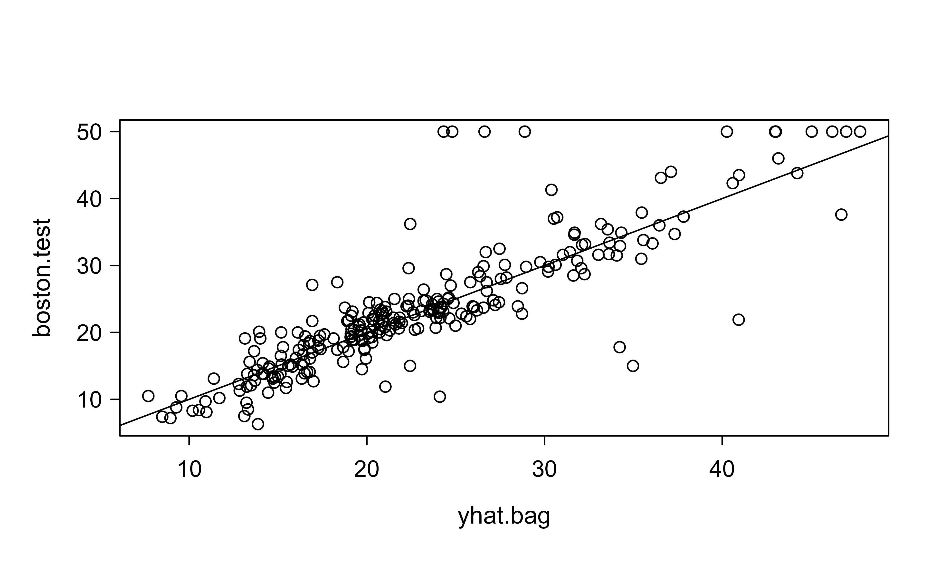
Now we evaluate the bagged model on the held-out test set. Figure 10.1 compares predicted values against the true test responses, and the 45-degree line marks perfect prediction.

Show code

yhat.bag <- predict(bag.boston, newdata = Boston[-train, ])
plot(yhat.bag, boston.test)
abline(0, 1)
mean((yhat.bag - boston.test) ^ 2) # test set MSE
#> [1] 23.40359

Figure 10.1: Predicted median home values from the bagged model plotted against the true test-set responses, with the 45-degree line marking perfect prediction.

Points hugging the line indicate accurate predictions. The reported number is the test-set MSE, our headline measure of how well the bagged model generalizes.

By default randomForest() grows 500 trees. We can change how many trees are grown with the ntree argument; here we shrink the ensemble to 25 trees to see the effect.

Show code

bag.boston <-
    randomForest(
        medv ~ . ,
        data = Boston,
        subset = train,
        mtry = 12,
        ntree = 25 # spceify number of grown tree
    )
yhat.bag <- predict(bag.boston, newdata = Boston[-train,])
mean((yhat.bag - boston.test) ^ 2)
#> [1] 24.59162

Tip

More trees rarely hurt accuracy and never cause overfitting in bagging, so the practical question is how many trees you can afford rather than how many you should risk. Fewer trees mainly trade away a little stability for faster computation.

10.5.1 Hyperparameters, cost, and diagnostics

Bagging has few knobs, which is part of its appeal. The choices that matter:

Number of trees $B$ (ntree). Not a complexity parameter. By Equation 10.1 the Monte Carlo part of the variance falls like $(1-\rho)\sigma^2/B$, so returns diminish quickly. Choose $B$ by watching the OOB error stabilize: plot(bag.boston) shows error against the number of trees, and you stop where the curve flattens. A few hundred trees is typical; use more only if you also need stable importance scores or OOB estimates.
Tree size. Grow deep, essentially unpruned trees (in randomForest, controlled by nodesize, default $5$ for regression and $1$ for classification, and maxnodes). Deep trees have low bias and high variance, and Equation 10.2 says the high variance is exactly what averaging removes. Pruning would reintroduce bias that averaging cannot fix.
mtry. Setting mtry = p gives pure bagging; values $m < p$ give a random forest. Because the variance floor in Equation 10.1 is $\rho\sigma^2$ and smaller $m$ lowers $\rho$, tuning mtry (by OOB error) is usually the single most effective adjustment, which is why random forests typically dominate plain bagging.

Computationally, training is $O(B \cdot n \log n \cdot p)$ for the trees (each tree sorts features at each level), trivially parallel across the $B$ trees since they are independent. Memory scales with the total number of nodes stored. Prediction is $O(B \cdot \text{depth})$ per query.

For diagnostics, prefer the OOB error of Equation 10.4 over a separate validation split when data is scarce, since it uses all observations. Compare the OOB MSE printed in the model summary against the held-out test MSE: large disagreement signals distribution shift between train and test, or too few trees making the OOB estimate noisy.

10.6 From bagging to random forests

Growing a random forest is a small twist on bagging: instead of considering all $p$ predictors at each split, we restrict each split to a random subset of $m < p$ predictors. This decorrelates the trees so the average is even more effective. The randomForest() defaults reflect common choices for $m$:

$\frac{p}{3}$ variables to build a random forest of regression trees (Chapter 8)
$\sqrt{p}$ variables to build a random forest of classification trees

Here we fit a regression random forest using mtry = 6 predictors at each split.

Show code

set.seed(1)
rf.boston <-
    randomForest(
        medv ~ . ,
        data = Boston,
        subset = train,
        mtry = 6,
        # use 6 variables
        importance = T
    )
yhat.rf <- predict(rf.boston, newdata = Boston[-train, ])
mean((yhat.rf - boston.test) ^ 2)
#> [1] 20.06644

The random forest improves on bagging here: its test MSE (about 20) is lower than the bagging MSE (about 25). Restricting the predictors at each split paid off by making the trees less alike, so their average generalizes better. Bagging and random forests build their trees independently and in parallel; an alternative ensemble strategy that grows trees sequentially, each correcting the errors of the last, is covered in the boosting chapter (Chapter 11).

10.7 Reading variable importance

Because we set importance = T, we can ask which predictors the forest relied on most.

Show code

importance(rf.boston)
#>           %IncMSE IncNodePurity
#> crim    19.435587    1070.42307
#> zn       3.091630      82.19257
#> indus    6.140529     590.09536
#> chas     1.370310      36.70356
#> nox     13.263466     859.97091
#> rm      35.094741    8270.33906
#> age     15.144821     634.31220
#> dis      9.163776     684.87953
#> rad      4.793720      83.18719
#> tax      4.410714     292.20949
#> ptratio  8.612780     902.20190
#> lstat   28.725343    5813.04833

The output has two columns, each summarizing importance from a different angle:

The mean decrease in prediction accuracy on the OOB samples when that variable’s values are scrambled.
The total decrease in node impurity from splits on that variable, averaged over all trees. For regression trees this is based on the training RSS, and for classification trees it is based on the deviance.

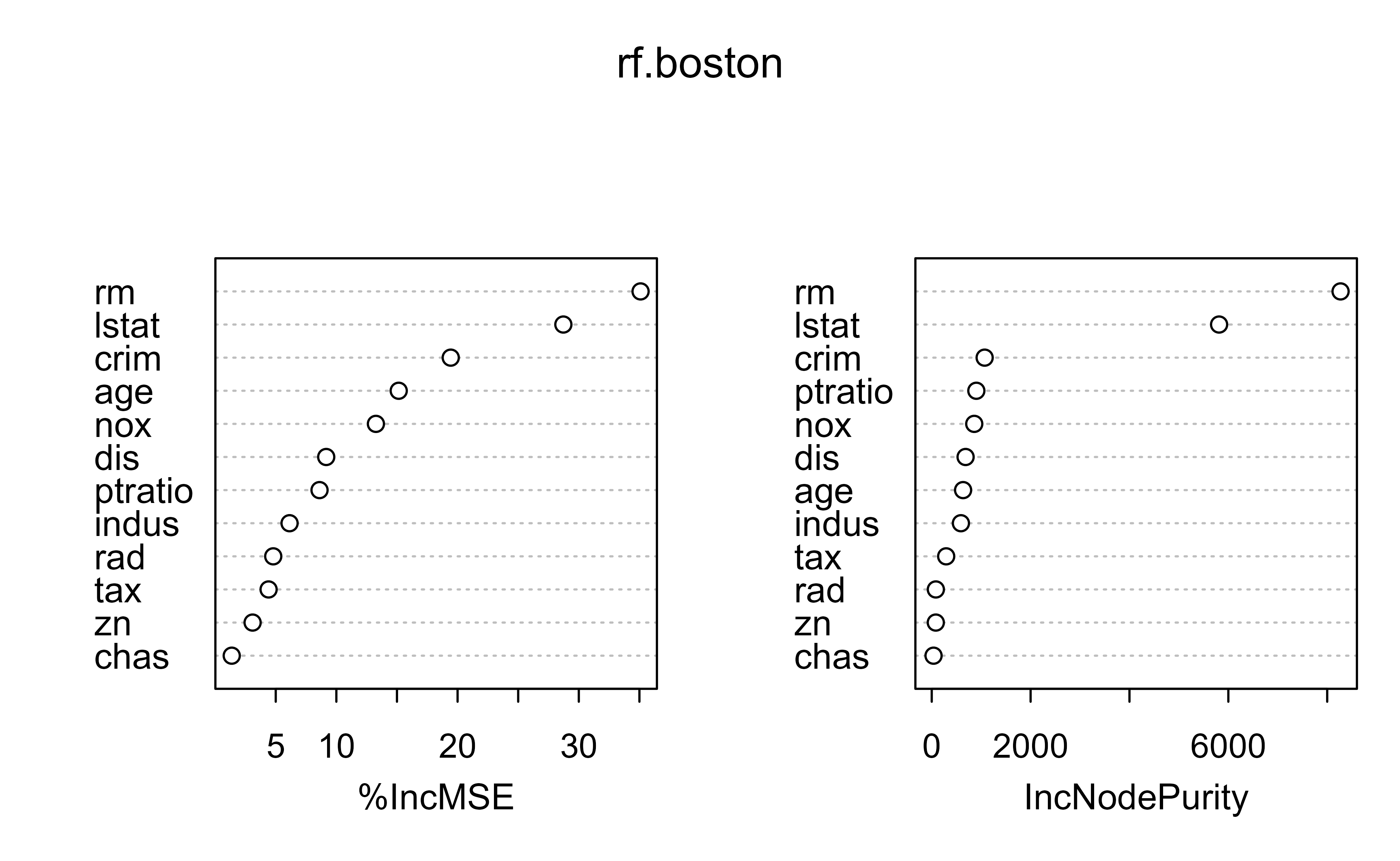
A picture makes the ranking easier to read than the raw table. Figure 10.2 displays the two importance measures side by side.

Show code

varImpPlot(rf.boston) #rm and lstate are most important

Figure 10.2: Variable importance for the random forest fit to the Boston housing data, showing the mean decrease in accuracy and the mean decrease in node impurity for each predictor.

Both panels point to the same conclusion: rm (average number of rooms) and lstat (percentage of lower-status population) are by far the most important predictors of median home value, which matches what we would expect from housing economics.

When to use this

Reach for bagging or a random forest whenever a single tree predicts well in spirit but is too unstable to trust, and you are willing to trade the readability of one tree for stronger, more reliable predictions. Variable importance plots then give you back a coarse, ensemble-level view of which predictors drive the model.

Although we apply it to trees here, bagging is not specific to trees. It can wrap around any base learner whose predictions are sensitive to the training sample.↩︎
On average, each bootstrap sample omits about one third of the original observations, so every observation is OOB for roughly a third of the trees, giving us plenty of trees to average over.↩︎

# Bagging {#sec-bagging} ```{r} #| include: false source("_common.R") ``` A single decision tree, like CART (see the classification and regression trees chapter, @sec-regression-trees) or MARS (@sec-mars), is easy to read but unstable. If you split your training data into two halves at random and grow a tree on each half, you can end up with two very different trees that make very different predictions. This sensitivity to the particular sample you happened to draw is what statisticians call high variance, and it is the main reason a lone tree often predicts poorly on new data. This chapter introduces a remedy called bagging, short for bootstrap aggregation. The idea is simple and powerful: instead of trusting one unstable tree, grow many trees on slightly different versions of the data and average their predictions. Averaging cancels out the random wobble of any individual tree, so the combined predictor is far more stable than its parts. By the end of the chapter you will understand why averaging reduces variance, how the bootstrap lets us mimic having many training sets when we really have only one, how to estimate test error for free using out-of-bag samples, and how to measure variable importance once the trees are no longer individually interpretable. Bagging is also the conceptual stepping stone to random forests (@sec-random-forest), which we preview here. ::: {.callout-tip title="Intuition"} Think of each tree as a noisy measurement of the same underlying quantity. One measurement is unreliable, but the average of many independent measurements is close to the truth. Bagging applies that everyday logic to prediction models. ::: ## Why averaging reduces variance Some procedures are naturally stable. Ordinary linear regression, for example, gives nearly the same fit whether you run it on one random sample or another, especially when the number of observations $n$ is large relative to the number of predictors $p$. A procedure with low variance yields similar results when applied repeatedly to distinct data sets. Trees are the opposite: they are flexible enough to chase noise, so small changes in the data produce large changes in the fitted model. Bagging is a general-purpose procedure for reducing the variance of any such unstable method.^[Although we apply it to trees here, bagging is not specific to trees. It can wrap around any base learner whose predictions are sensitive to the training sample.] The strategy is to average many models. If we had access to $B$ separate training sets, we could fit a model on each, call them $\hat{f}^1(X), \hat{f}^2(X), \dots, \hat{f}^B(X)$, and average them into a single bagged predictor: $$ \hat{f}_{bag} (X) = \frac{1}{B} \sum_{b=1}^B \hat{f}^b (x) $$ ::: {.callout-important title="Key idea"} Averaging keeps the bias of the base model roughly the same while shrinking its variance. That is why we deliberately grow each tree large and unpruned: large trees have low bias but high variance, and averaging takes care of the variance. ::: ### The variance-reduction identity {#sec-bagging-variance} Fix a test point $x$ and treat each base prediction $\hat f^b(x)$ as a random variable, with the randomness coming from the training sample (and, for bootstrap bagging, from the resampling). Suppose the $B$ predictors are identically distributed, each with mean $\mu(x) = \mathbb{E}[\hat f^b(x)]$ and variance $\sigma^2(x) = \operatorname{Var}(\hat f^b(x))$, and with a common pairwise correlation $$ \rho(x) \;=\; \operatorname{Corr}\!\big(\hat f^b(x),\,\hat f^{b'}(x)\big), \qquad b \neq b'. $$ The bagged predictor is the average $\hat f_{bag}(x) = \tfrac{1}{B}\sum_b \hat f^b(x)$. Its mean is unchanged, $\mathbb{E}[\hat f_{bag}(x)] = \mu(x)$, so bagging does not alter bias under this model. For the variance, expand the variance of a sum: $$ \operatorname{Var}\!\Big(\tfrac{1}{B}\textstyle\sum_{b=1}^B \hat f^b(x)\Big) = \frac{1}{B^2}\Big[\sum_{b=1}^B \operatorname{Var}(\hat f^b) + \sum_{b\neq b'}\operatorname{Cov}(\hat f^b,\hat f^{b'})\Big]. $$ There are $B$ variance terms each equal to $\sigma^2$, and $B(B-1)$ covariance terms each equal to $\rho\sigma^2$. Substituting, $$ \operatorname{Var}(\hat f_{bag}(x)) = \frac{1}{B^2}\big[B\sigma^2 + B(B-1)\rho\sigma^2\big] = \rho\,\sigma^2 + \frac{1-\rho}{B}\,\sigma^2 . $$ {#eq-bagging-varbag} @eq-bagging-varbag is the central theoretical fact about bagging. Read it term by term: - As $B \to \infty$ the second term vanishes, leaving the floor $\rho\sigma^2$. You cannot average away the part of the variance that the trees share. This is exactly why decorrelating the trees, by sampling a subset of $m < p$ predictors at each split, lowers the floor and motivates random forests (@sec-random-forest). - If the predictors were independent ($\rho = 0$) the variance would collapse to $\sigma^2/B$, the classical $1/B$ rate for averaging i.i.d. quantities. Bootstrap samples overlap heavily, so in practice $\rho$ is well above zero and most of the gain is realized within the first one to two hundred trees. ::: {.callout-note} The decomposition assumes a common correlation $\rho \ge 0$, which holds for bootstrap-trained trees because they share the same underlying data. Adding trees can only reduce $\operatorname{Var}(\hat f_{bag})$ toward the floor $\rho\sigma^2$; it never increases it. This is the precise sense in which "more trees never overfit" in bagging: $B$ is a smoothing parameter for the Monte Carlo average, not a model-complexity knob. ::: ### Why bagging helps unstable learners and can hurt stable ones {#sec-bagging-jensen} Variance reduction is not a free lunch for every base learner. Consider the idealized aggregated predictor that averages over the true sampling distribution of the data, $f_{A}(x) = \mathbb{E}_{\mathcal D}[\hat f(x;\mathcal D)]$, where $\mathcal D$ is a training set of size $n$. For squared-error loss with a fixed target $y$, expand around $f_A$: $$ \mathbb{E}_{\mathcal D}\big[(y - \hat f(x;\mathcal D))^2\big] = (y - f_A(x))^2 + \mathbb{E}_{\mathcal D}\big[(\hat f(x;\mathcal D) - f_A(x))^2\big] \ge (y - f_A(x))^2 . $$ {#eq-bagging-jensen} The cross term cancels because $\mathbb{E}_{\mathcal D}[\hat f - f_A] = 0$, and the remaining term is the variance of the base learner. @eq-bagging-jensen says the aggregated predictor's squared error never exceeds the average squared error of the base learner, and the gap is precisely the variance. The more variable (unstable) the learner, the larger the improvement; for a perfectly stable learner the gap is zero and bagging does nothing. Bagging approximates $f_A$ by the bootstrap average, so it inherits this behavior: large gains for high-variance learners like deep trees, negligible or even slightly negative effects for low-variance learners like linear regression, because the bootstrap approximation introduces its own small error. ::: {.callout-warning} For classification the squared-error argument does not transfer directly, and voting can in rare cases make a good classifier worse. If the base classifier is already better than random in a region, majority voting pushes its accuracy toward $1$ there; but in regions where it is worse than random, voting amplifies the error toward $0$. Bagging therefore helps "order-correct" classifiers and can degrade poor ones. In practice with reasonable trees this almost never bites, but it explains why bagging is not universally beneficial. ::: ## The bootstrap: many data sets from one There is a practical problem with the recipe above. In reality we almost never have $B$ independent training sets; we have a single sample. The bootstrap solves this by manufacturing surrogate data sets from the one we have. To create a bootstrap sample, we draw observations from the original training set at random with replacement until we have a data set of the same size. Because we sample with replacement, some observations appear more than once and others not at all, so each bootstrap sample differs slightly from the original. We generate $B$ such bootstrap samples, fit a model on each, and average the fits. The bagged prediction $\hat{f}_{bag}(x)$ is the average of the fits from these $B$ bootstrap samples, exactly as in the formula above but with bootstrap samples standing in for genuine independent training sets. ### How much of the data does a bootstrap sample see? {#sec-bagging-omission} The "roughly one third left out" figure quoted below is not a rule of thumb but an exact limit. A bootstrap sample is drawn by taking $n$ independent draws, each uniform over the $n$ training indices. The probability that a particular observation $i$ is missed on a single draw is $1 - \tfrac{1}{n}$, and since the draws are independent the probability it is missed on all $n$ draws is $$ \Pr(i \notin \text{bootstrap sample}) = \Big(1 - \frac{1}{n}\Big)^{n}. $$ {#eq-bagging-oob} Using $\big(1 - \tfrac{1}{n}\big)^{n} = \exp\!\big[n\ln(1 - \tfrac1n)\big]$ and the expansion $\ln(1 - \tfrac1n) = -\tfrac1n - \tfrac{1}{2n^2} - \cdots$, the exponent tends to $-1$, so $$ \lim_{n\to\infty}\Big(1 - \frac{1}{n}\Big)^{n} = e^{-1} \approx 0.368 . $$ About $36.8\%$ of observations are out-of-bag for any given tree, and the complementary $\approx 63.2\%$ are in-bag (the distinct observations appearing at least once; of these, about $36.8\%$ of all observations appear exactly once and about $26.4\%$ appear more than once). The convergence is fast: even at $n = 20$ the omission probability is $0.358$. This single number underlies both the out-of-bag error estimate below and the effective training-set size each tree sees. ::: {.callout-note} With regression trees, we construct $B$ trees and average their predictions, growing each tree large with no pruning. Each tree on its own has high variance and low bias; averaging then drives the variance down without inflating the bias. In practice, around **100** trees is usually enough to capture most of the variance reduction. ::: For classification the averaging step changes slightly because we cannot average class labels directly. Instead, we record the class predicted by each of the $B$ trees for a given test observation and take a majority vote, choosing the category that occurs most often across the trees. ## Out-of-bag error: cross-validation for free A pleasant side effect of the bootstrap is that we can estimate test error without performing cross-validation. The reason is that each bootstrap sample leaves some observations out by construction. The procedure works as follows. For a given tree, the observations that were not selected into its bootstrap sample are called the out-of-bag (OOB) observations for that tree.^[On average, each bootstrap sample omits about one third of the original observations, so every observation is OOB for roughly a third of the trees, giving us plenty of trees to average over.] To get an OOB prediction for the $i$-th observation, we use only the trees in which that observation was OOB, and average their predictions. Comparing these OOB predictions against the true responses gives the OOB MSE for regression, or the OOB classification error for classification. Formally, let $O_i = \{\, b : i \notin \text{bootstrap sample } b \,\}$ be the set of trees for which observation $i$ is out-of-bag. The OOB prediction and the OOB error estimate are $$ \hat f^{\,\text{oob}}(x_i) = \frac{1}{|O_i|}\sum_{b \in O_i} \hat f^b(x_i), \qquad \widehat{\text{Err}}_{\text{oob}} = \frac{1}{n}\sum_{i=1}^n L\big(y_i,\, \hat f^{\,\text{oob}}(x_i)\big), $$ {#eq-bagging-ooberr} with $L$ the squared error for regression or the $0/1$ loss (via the OOB majority vote) for classification. Because each $\hat f^{\,\text{oob}}(x_i)$ averages over only $|O_i| \approx 0.368\,B$ trees, the OOB estimate for a forest of $B$ trees behaves like a test estimate for a smaller forest of about $0.368\,B$ trees; it is therefore mildly pessimistic when $B$ is small, and the bias disappears as $B$ grows. The OOB estimate is nearly equivalent to leave-one-out cross-validation but costs nothing extra, since the trees are already fit. Its main limitation is that the $\hat f^{\,\text{oob}}(x_i)$ are not independent across $i$ (they share trees), so the OOB error has no simple standard error. ::: {.callout-important title="Key idea"} The OOB error is a valid estimate of the test error because each observation is predicted only by trees that never saw it during training. No data point judges a model that was trained on it. ::: We can confirm the omission probability of @eq-bagging-oob and the resulting OOB share by direct simulation. ```{r} set.seed(1) n <- 200 B <- 2000 in_bag <- replicate(B, sort(unique(sample(1:n, n, replace = TRUE)))) oob_fraction <- mean(sapply(in_bag, function(s) (n - length(s)) / n)) c(simulated = oob_fraction, theoretical = (1 - 1/n)^n, limit = exp(-1)) ``` The simulated out-of-bag fraction matches $(1 - 1/n)^n$ and its limit $e^{-1}$. ## The cost: losing interpretability Bagging buys predictive accuracy, but it gives up the clarity that made a single tree appealing. A lone tree can be drawn as a flowchart and read top to bottom. Once we average over hundreds of trees, the variable used at each split (or the basis function included) can change dramatically from tree to tree, so there is no single diagram to interpret and no obvious way to say which variable matters most. To recover some interpretation, we track how much each predictor contributes to the trees, averaged over all $B$ of them. The two standard measures of variable importance are: - For regression, the total amount by which the residual sum of squares is decreased due to splits on a given predictor, averaged over all $B$ trees. - For classification, the total amount by which the Gini index is decreased by splits on a given predictor, averaged over all $B$ trees. A predictor that consistently produces large reductions in error across the ensemble is judged important, even though we can no longer point to a single tree to explain why. Variable importance is one of several tools for understanding otherwise opaque models, a topic taken up more broadly in the interpretable machine learning chapter (@sec-interpretable-machine-learning). ### Two importance measures, made precise {#sec-bagging-importance} The `randomForest` output reports two distinct quantities, and it is worth stating each exactly because they can disagree. **Impurity (Gini / RSS) importance.** When a split on variable $j$ at node $t$ in tree $b$ reduces node impurity by $\Delta i_t$ (the drop in RSS for regression, or in the Gini index $G_t = \sum_k \hat p_{tk}(1 - \hat p_{tk})$ for classification), accumulate that decrease. The importance of $X_j$ is the total over all nodes that split on $j$, averaged over trees: $$ \text{Imp}^{\text{imp}}(X_j) = \frac{1}{B}\sum_{b=1}^B \;\sum_{t \in T_b\,:\, v(t)=j} \Delta i_t , $$ {#eq-bagging-impgini} where $v(t)$ is the variable used at node $t$. This is computed for free during training but is known to be biased toward variables with many possible split points (continuous or high-cardinality categorical predictors), because such variables get more chances to reduce impurity by chance. **Permutation (mean-decrease-in-accuracy) importance.** For each tree $b$, compute the OOB error $e_b$. Then randomly permute the values of $X_j$ among the OOB observations, breaking the association between $X_j$ and $y$ while preserving its marginal distribution, and recompute the OOB error $e_b^{(j)}$. The importance is the average increase in error: $$ \text{Imp}^{\text{perm}}(X_j) = \frac{1}{B}\sum_{b=1}^B \big(e_b^{(j)} - e_b\big). $$ {#eq-bagging-impperm} This is model-agnostic in spirit and far less biased by cardinality, but it is more expensive (one extra OOB pass per variable) and is itself biased when predictors are strongly correlated: permuting one of two collinear predictors leaves the information available through the other, so both can look unimportant. Conditional permutation schemes address this. ::: {.callout-warning} Do not over-interpret a single importance ranking. Impurity importance inflates high-cardinality variables, and permutation importance splits credit between correlated predictors. When two predictors carry the same signal, the ensemble may rely on either, so their individual importances can be unstable across reruns even when their joint contribution is large. ::: ## Bagging in R Bagging is a special case of a random forest in which every predictor is a candidate at every split. Concretely, bagging corresponds to a random forest with $m = p$, where $m$ is the number of input variables considered at each split and $p$ is the number of available variables. Because of this, we can carry out bagging with the `randomForest()` function simply by setting `mtry` equal to the total number of predictors. We illustrate with the `Boston` housing data, predicting median home value `medv`. We first split the data in half to create a training set and a test set. ```{r, message=FALSE, warning=FALSE} library(randomForest) library(ISLR2) library(tree) set.seed(1) train <- sample(1:nrow(Boston), nrow(Boston)/2) boston.test <- Boston[-train, "medv"] bag.boston <- randomForest( medv ~ ., data = Boston, subset = train, mtry = 12, # all 12 predcitors should be used for each split of the tree importance = T ) # we could use random forest because bagging is a special case of random forest with m = p bag.boston ``` Setting `mtry = 12` tells the function to consider all 12 predictors at every split, which is exactly what makes this bagging rather than a random forest. The printed summary reports the type of forest, the number of trees, and the percentage of variance explained on the out-of-bag samples. Now we evaluate the bagged model on the held-out test set. @fig-bagging-pred-vs-actual compares predicted values against the true test responses, and the 45-degree line marks perfect prediction. ```{r fig-bagging-pred-vs-actual, fig.cap="Predicted median home values from the bagged model plotted against the true test-set responses, with the 45-degree line marking perfect prediction."} yhat.bag <- predict(bag.boston, newdata = Boston[-train, ]) plot(yhat.bag, boston.test) abline(0, 1) mean((yhat.bag - boston.test) ^ 2) # test set MSE ``` Points hugging the line indicate accurate predictions. The reported number is the test-set MSE, our headline measure of how well the bagged model generalizes. By default `randomForest()` grows 500 trees. We can change how many trees are grown with the `ntree` argument; here we shrink the ensemble to 25 trees to see the effect. ```{r} bag.boston <- randomForest( medv ~ . , data = Boston, subset = train, mtry = 12, ntree = 25 # spceify number of grown tree ) yhat.bag <- predict(bag.boston, newdata = Boston[-train,]) mean((yhat.bag - boston.test) ^ 2) ``` ::: {.callout-tip} More trees rarely hurt accuracy and never cause overfitting in bagging, so the practical question is how many trees you can afford rather than how many you should risk. Fewer trees mainly trade away a little stability for faster computation. ::: ### Hyperparameters, cost, and diagnostics {#sec-bagging-howto} Bagging has few knobs, which is part of its appeal. The choices that matter: - **Number of trees $B$ (`ntree`).** Not a complexity parameter. By @eq-bagging-varbag the Monte Carlo part of the variance falls like $(1-\rho)\sigma^2/B$, so returns diminish quickly. Choose $B$ by watching the OOB error stabilize: `plot(bag.boston)` shows error against the number of trees, and you stop where the curve flattens. A few hundred trees is typical; use more only if you also need stable importance scores or OOB estimates. - **Tree size.** Grow deep, essentially unpruned trees (in `randomForest`, controlled by `nodesize`, default $5$ for regression and $1$ for classification, and `maxnodes`). Deep trees have low bias and high variance, and @eq-bagging-jensen says the high variance is exactly what averaging removes. Pruning would reintroduce bias that averaging cannot fix. - **`mtry`.** Setting `mtry = p` gives pure bagging; values $m < p$ give a random forest. Because the variance floor in @eq-bagging-varbag is $\rho\sigma^2$ and smaller $m$ lowers $\rho$, tuning `mtry` (by OOB error) is usually the single most effective adjustment, which is why random forests typically dominate plain bagging. Computationally, training is $O(B \cdot n \log n \cdot p)$ for the trees (each tree sorts features at each level), trivially parallel across the $B$ trees since they are independent. Memory scales with the total number of nodes stored. Prediction is $O(B \cdot \text{depth})$ per query. For diagnostics, prefer the OOB error of @eq-bagging-ooberr over a separate validation split when data is scarce, since it uses all observations. Compare the OOB MSE printed in the model summary against the held-out test MSE: large disagreement signals distribution shift between train and test, or too few trees making the OOB estimate noisy. ## From bagging to random forests Growing a random forest is a small twist on bagging: instead of considering all $p$ predictors at each split, we restrict each split to a random subset of $m < p$ predictors. This decorrelates the trees so the average is even more effective. The `randomForest()` defaults reflect common choices for $m$: - $\frac{p}{3}$ variables to build a random forest of regression trees (@sec-regression-trees) - $\sqrt{p}$ variables to build a random forest of classification trees Here we fit a regression random forest using `mtry = 6` predictors at each split. ```{r} set.seed(1) rf.boston <- randomForest( medv ~ . , data = Boston, subset = train, mtry = 6, # use 6 variables importance = T ) yhat.rf <- predict(rf.boston, newdata = Boston[-train, ]) mean((yhat.rf - boston.test) ^ 2) ``` The random forest improves on bagging here: its test MSE (about 20) is lower than the bagging MSE (about 25). Restricting the predictors at each split paid off by making the trees less alike, so their average generalizes better. Bagging and random forests build their trees independently and in parallel; an alternative ensemble strategy that grows trees sequentially, each correcting the errors of the last, is covered in the boosting chapter (@sec-boosting). ## Reading variable importance Because we set `importance = T`, we can ask which predictors the forest relied on most. ```{r} importance(rf.boston) ``` The output has two columns, each summarizing importance from a different angle: 1. The mean decrease in prediction accuracy on the OOB samples when that variable's values are scrambled. 2. The total decrease in node impurity from splits on that variable, averaged over all trees. For regression trees this is based on the training RSS, and for classification trees it is based on the deviance. A picture makes the ranking easier to read than the raw table. @fig-bagging-var-importance displays the two importance measures side by side. ```{r fig-bagging-var-importance, fig.cap="Variable importance for the random forest fit to the Boston housing data, showing the mean decrease in accuracy and the mean decrease in node impurity for each predictor."} varImpPlot(rf.boston) #rm and lstate are most important ``` Both panels point to the same conclusion: `rm` (average number of rooms) and `lstat` (percentage of lower-status population) are by far the most important predictors of median home value, which matches what we would expect from housing economics. ::: {.callout-tip title="When to use this"} Reach for bagging or a random forest whenever a single tree predicts well in spirit but is too unstable to trust, and you are willing to trade the readability of one tree for stronger, more reliable predictions. Variable importance plots then give you back a coarse, ensemble-level view of which predictors drive the model. :::