Most of this book studies models whose parameters you fit. With a pretrained large language model (LLM) you usually do not fit parameters at all. You shape behavior by what you put in the context window: instructions, examples, and a specification of the output you want back. Prompt engineering is the discipline of designing that input so the model produces useful, parseable, reliable results. Structured output is the part of that discipline that forces the model to answer in a machine-readable format (typically JSON) so the result can flow into the rest of a data pipeline.
Here is the intuition before any formalism. Think of a pretrained LLM as a fixed function that takes a block of text in and produces a block of text out. You cannot reach inside and retune it, but you can decide exactly what text goes in, and you can decide how adventurous the model is allowed to be when it writes the output. Those are the only two dials you have, and almost everything in this chapter is a careful use of one of them. The reward for using them well is large: a task that would normally need a labeled dataset and a training run can often be solved by writing a few paragraphs of instructions and reading back a small, well-shaped result.
This chapter treats prompting as a design problem with measurable trade-offs, not folklore. We define the objects (system prompt, user prompt, few-shot examples, tool schemas), give the probabilistic meaning of the decoding parameters that control randomness (temperature and top-\(p\)), and show why asking for JSON and then validating it is the difference between a demo and a production component. By the end you will be able to read a prompt as a program, explain in probabilistic terms what temperature does to the output, and turn a chatty text generator into something a downstream job can call like a typed function. The runnable demonstration is implemented in base R plus glue: a prompt-template function that assembles a few-shot prompt from a table of examples, plus a small JSON-schema validator that checks whether a model’s (simulated) reply conforms to the contract you asked for.1
Key idea
With a frozen LLM you never change the model. You change its input (the prompt) and you change how you sample from its output (the decoding parameters). Hold on to that distinction and the rest of the chapter is just two levers.
109.1 Where this fits in a modern ML/AI workflow
In a classical supervised pipeline you collect labels, train a model, and serve it. With a capable instruction-tuned LLM you often skip training entirely for a first version of a task: classification, extraction, summarization, routing, and data cleaning can be done by describing the task in a prompt and reading back structured fields. The prompt is the program.
This matters for a data team in three concrete ways. The first is speed to a baseline: a zero-shot or few-shot prompt is a working baseline in minutes, before anyone labels a training set, and it tells you almost immediately whether the task is even well posed. The second is that structured output acts as an API contract. If the model returns free text, a human has to read it; if it returns JSON that matches a fixed schema, a downstream job can consume it like any other service. Validation is what turns a stochastic text generator into a typed function. The third is that prompting sits at the bottom of a clean fallback ladder. Prompting, few-shot prompting, retrieval (Chapter 111), tool use (Chapter 112), and fine-tuning are not competitors but rungs you climb only when the cheaper rung fails its evaluation. Prompt engineering is the rung you should exhaust first.
When to use this
Start with a prompt whenever the task can be described in words and the base model is already good at the underlying skill. Climb to retrieval or fine-tuning only after a held-out evaluation shows the prompt has plateaued below your target. Cheaper rungs first, always.
The mental model for the rest of the chapter: an LLM defines a conditional distribution over output tokens given the input tokens, \(p_\theta(y \mid x)\) with frozen parameters \(\theta\). You do not change \(\theta\). You change \(x\) (the prompt) and you change how you sample from \(p_\theta(\cdot \mid x)\) (the decoding parameters). Everything below is one of those two levers.
109.2 The anatomy of a prompt
Before we can shape a prompt, we need names for its parts. Modern chat models accept a list of messages, each tagged with a role, and you control three of them. The system prompt holds persistent instructions that set the model’s task, tone, constraints, and output format; it is read once and conditions everything after it, so this is where the contract belongs (“You are a classifier. Return only JSON matching this schema.”). The user prompt is the specific request or input to act on, for example the one document you want classified. Assistant messages are the model’s replies, and you can also fabricate them to supply worked examples (few-shot), where each example is a user turn followed by the ideal assistant turn.
Tip
The split between system and user prompts is the split between “rules that hold for every call” and “the one item this call is about.” Putting the output schema in the system prompt and the data in the user prompt keeps the contract stable while the input varies.
Formally, the input \(x\) is the concatenation of the rendered messages, \(x = \texttt{render}(m_1, \dots, m_k)\), where each \(m_i = (\text{role}_i,
\text{content}_i)\). The model never sees roles as anything magical; they are special tokens in \(x\).2 The practical consequence is that the order and labeling of content changes the conditional distribution, which is why moving an instruction from the user turn into the system turn can change behavior.
109.2.1 Zero-shot, few-shot, and chain-of-thought
Three prompting patterns cover most applied use, and they differ only in what extra content you place in \(x\). Zero-shot prompting describes the task, gives the input, and asks for the answer, with no examples at all; it works when the task is common and the instruction is unambiguous. Few-shot prompting prepends \(n\) solved examples \((u_1, a_1), \dots, (u_n, a_n)\) before the real input \(u^\*\), so the examples teach the format and the decision boundary by demonstration. This is in-context learning: the model adapts its behavior from examples in the prompt with no weight update (Brown et al., 2020). Chain-of-thought (CoT) prompting asks the model to produce intermediate reasoning steps before the final answer (Wei et al., 2022); for multi-step problems such as arithmetic, logic, or multi-hop questions this raises accuracy, because the intermediate tokens give the autoregressive model a scratchpad, and later tokens condition on the reasoning it already wrote.
Intuition
A model generates one token at a time, each conditioned on everything before it. Letting it “think out loud” first means the final answer is generated in the presence of useful intermediate work, rather than being guessed in a single leap. The scratchpad is the point.
There is a real tension between CoT and structured output. Free-form reasoning is text, not JSON. The standard resolution is to keep the reasoning inside a field of the JSON object, for example a "reasoning" string emitted before the "answer" field, so you get the accuracy benefit and a parseable result. The ordering matters: because generation is left to right, the model must write the reasoning field first for it to actually inform the answer field.
109.3 Decoding parameters: the probabilistic view
We have talked about changing the input \(x\). The second lever is how you draw the output from \(p_\theta(\cdot \mid x)\), and it is controlled by a handful of decoding parameters. The intuition is simple: the model assigns a score to every possible next word, and these parameters decide whether you always take the top-scoring word or occasionally gamble on a lower-scoring one. Taking the top word every time is repeatable and safe; gambling adds variety at the cost of reliability. The math below just makes “gamble how much” precise.
At each step the model produces a vector of logits \(z \in \mathbb{R}^{V}\) over a vocabulary of size \(V\).3 The next-token distribution is a softmax of those logits scaled by the temperature \(\tau > 0\):
\[
p_\tau(v) = \frac{\exp(z_v / \tau)}{\sum_{u=1}^{V} \exp(z_u / \tau)}, \qquad v = 1, \dots, V.
\]
Temperature reshapes the same logits without retraining anything.
As \(\tau \to 0^{+}\) the distribution concentrates on \(\arg\max_v z_v\). Sampling becomes deterministic and equals greedy decoding.
At \(\tau = 1\) you sample from the model’s native distribution.
As \(\tau\) grows the distribution flattens toward uniform, so rare tokens get more mass and output gets more diverse and less reliable.
A useful way to quantify “how flat” the distribution is is the entropy \(H(p_\tau) = -\sum_v p_\tau(v) \log p_\tau(v)\), which increases monotonically with \(\tau\) from \(0\) (a point mass) toward \(\log V\) (uniform). You can read entropy here as a single number summarizing how undecided the model is at this step: low entropy means it is confident in one token, high entropy means many tokens look roughly equally good.
Top-\(p\) (nucleus) sampling truncates the tail before sampling (Holtzman et al., 2020). Sort tokens by probability and keep the smallest set \(\mathcal{N}_p\) whose cumulative mass first reaches \(p\):
then renormalize over \(\mathcal{N}_p\) and sample. Setting \(p = 1\) disables truncation; small \(p\) removes the long tail of implausible tokens while still allowing variety among the plausible ones. Top-\(k\) is the same idea but keeps a fixed count \(k\) of highest-probability tokens regardless of their mass.
The practical rule that follows from the math: for tasks with a single correct answer (classification, extraction, anything you will parse), push \(\tau\) toward \(0\) so the output is near-deterministic and reproducible. For open-ended generation where you want variety (brainstorming, drafting), raise \(\tau\) and use top-\(p\) around \(0.9\) to cut the worst tail.
Warning
Any temperature above \(0\) makes the output irreproducible. The same prompt can give different answers on different runs, which turns bugs into intermittent ghosts and makes evaluation noisy. If you are going to parse the result, decode cold.
Table 109.1 summarizes the levers. Read it as a quick-reference card: each row is one knob, what it controls, and which direction to turn it.
Table 109.1: Decoding parameters that control how output is sampled from the model, the quantity each one affects, and the direction to turn each knob for reliable parsing versus open-ended generation.
Parameter
Symbol
Range
Effect
When to lower
When to raise
Temperature
\(\tau\)
\((0, \infty)\)
scales logits before softmax
parsing, classification, reproducibility
brainstorming, creative drafts
Top-\(p\) (nucleus)
\(p\)
\((0, 1]\)
keep smallest set reaching mass \(p\)
factual or structured output
diverse generation
Top-\(k\)
\(k\)
\(\{1, 2, \dots\}\)
keep \(k\) highest-probability tokens
tighten output
widen candidate set
Max tokens
\(\{1, 2, \dots\}\)
hard cap on output length
control cost and latency
long reasoning or documents
Stop sequences
strings
end generation on a marker
enforce clean boundaries
rarely
109.4 Structured output and JSON schemas
So far we have shaped the input and tuned the sampling. The last piece is shaping the output, because a free-text answer is hard to consume programmatically. The fix is to specify the exact shape of the output and ask the model to return only that. A JSON schema is a declarative description of an object: its fields, their types, which are required, and any value constraints (for example an enumeration of allowed labels).4 You put the schema (or a compact description of it) in the system prompt, and you validate the model’s reply against it after generation.
Two failure modes make validation non-optional. The first is format drift: the model wraps the JSON in prose (“Here is the result:”) or in Markdown code fences, so you must extract the JSON substring before parsing. The second is a schema violation: the JSON parses cleanly but a required field is missing, a type is wrong, or a label is outside the allowed set, and only schema validation catches this.
Warning
Valid JSON is not the same as correct JSON. A reply can parse perfectly and still carry a label your pipeline has never heard of. Parsing without validating is the single most common way an LLM component silently corrupts the data downstream of it.
The contract, then, is a short sequence: parse, then validate, then act. If validation fails you retry with a corrective message, lower the temperature, or fall back to a default record. Production LLM services also offer constrained decoding that guarantees syntactically valid JSON, but valid JSON is not the same as schema-conformant JSON, so you still validate the fields. The demo below implements parse and validate from scratch so the moving parts are visible.
109.4.1 Function and tool schemas
Tool use generalizes structured output. Instead of returning a final answer, the model returns a structured call to a named function whose argument shape is itself a JSON schema you provide. The model picks the function and fills the arguments; your code executes it and feeds the result back.5 A weather assistant might expose a get_weather(location: string, unit: enum["C","F"]) tool; the model emits {"name": "get_weather", "arguments": {"location": "Paris", "unit": "C"}}. From the model’s side this is the same skill as structured output: emit JSON that matches a declared schema. The only new piece is that you, not the model, decide what to do with the validated arguments.
109.5 Prompt templates: the runnable demo
A prompt template is a string with named slots that you fill from data. Keeping templates as functions (rather than pasting strings) makes prompts versionable, testable, and consistent across thousands of calls. The demo builds a few-shot sentiment classifier prompt from a table of labeled examples, then validates a (simulated) model reply against a JSON schema. We do not call a paid API here; a small deterministic stub stands in for the model so the chapter is fully runnable and reproducible. Swapping the stub for a real client is a one-line change shown at the end.
Show code
suppressPackageStartupMessages(library(glue))suppressPackageStartupMessages(library(jsonlite))set.seed(1301)# Few-shot examples: an input text and its gold label.examples<-data.frame( text =c("This product exceeded my expectations.","Worst purchase I have ever made.","It works, nothing special either way."), label =c("positive", "negative", "neutral"), stringsAsFactors =FALSE)# The allowed labels define the enum constraint in our schema.allowed_labels<-c("positive", "negative", "neutral")
The template function renders a system prompt that states the contract, a block of few-shot examples, and the new input. Using glue keeps the slots explicit.
Show code
render_examples<-function(ex){# One example per shot: a user line then the ideal JSON assistant line.lines<-vapply(seq_len(nrow(ex)), function(i){gold<-toJSON(list(reasoning ="stated explicitly in the text", label =ex$label[i]), auto_unbox =TRUE)glue("Input: {ex$text[i]}\nOutput: {gold}")}, character(1))paste(lines, collapse ="\n\n")}build_prompt<-function(new_text, ex, labels){system_prompt<-glue("You are a sentiment classifier. Read the input text and return ONLY a ","JSON object with two fields: \"reasoning\" (a short string written first) ","and \"label\" (one of: {paste(labels, collapse = ', ')}). ","Do not add any text outside the JSON.")shots<-render_examples(ex)user_prompt<-glue("Input: {new_text}\nOutput:")list(system =as.character(system_prompt), user =paste(shots, user_prompt, sep ="\n\n"))}prompt<-build_prompt("Absolutely fantastic, I love it.",examples, allowed_labels)cat(prompt$system, "\n\n---\n\n", prompt$user, sep ="")#> You are a sentiment classifier. Read the input text and return ONLY a JSON object with two fields: "reasoning" (a short string written first) and "label" (one of: positive, negative, neutral). Do not add any text outside the JSON.#> #> ---#> #> Input: This product exceeded my expectations.#> Output: {"reasoning":"stated explicitly in the text","label":"positive"}#> #> Input: Worst purchase I have ever made.#> Output: {"reasoning":"stated explicitly in the text","label":"negative"}#> #> Input: It works, nothing special either way.#> Output: {"reasoning":"stated explicitly in the text","label":"neutral"}#> #> Input: Absolutely fantastic, I love it.#> Output:
Next, the JSON-schema validator. We define the schema as an R list and check a parsed object field by field: required presence, type, and (for label) the allowed enumeration. This is the same logic a production schema validator applies, written out so each check is visible.
Show code
# Schema: required fields, their JSON types, and optional enum constraints.schema<-list( reasoning =list(type ="string", required =TRUE), label =list(type ="string", required =TRUE, enum =allowed_labels))json_type<-function(x){if(is.logical(x))return("boolean")if(is.numeric(x))return("number")if(is.character(x))return("string")if(is.list(x))return("object")"unknown"}extract_json<-function(txt){# Strip code fences and surrounding prose: keep the first {...} block.m<-regmatches(txt, regexpr("\\{.*\\}", txt, perl =TRUE))if(length(m)==0)NA_character_elsem}validate_against<-function(obj, schema){errs<-character(0)for(fieldinnames(schema)){spec<-schema[[field]]if(is.null(obj[[field]])){if(isTRUE(spec$required))errs<-c(errs, glue("missing required field '{field}'"))next}if(json_type(obj[[field]])!=spec$type)errs<-c(errs, glue("field '{field}' has type ","'{json_type(obj[[field]])}', expected '{spec$type}'"))if(!is.null(spec$enum)&&!(obj[[field]]%in%spec$enum))errs<-c(errs, glue("field '{field}' value '{obj[[field]]}' ","not in allowed set"))}list(valid =length(errs)==0, errors =errs)}# End to end: take raw model text, extract JSON, parse, validate.process_reply<-function(raw_text, schema){js<-extract_json(raw_text)if(is.na(js))return(list(valid =FALSE, errors ="no JSON found", obj =NULL))obj<-tryCatch(fromJSON(js, simplifyVector =TRUE), error =function(e)NULL)if(is.null(obj))return(list(valid =FALSE, errors ="JSON did not parse", obj =NULL))res<-validate_against(obj, schema)c(res, list(obj =obj))}
Now a deterministic model stub. A real LLM is stochastic; here we mimic three realistic reply styles so we can exercise the validator: a clean reply, a reply wrapped in prose and a code fence, and a reply with an out-of-schema label.
The clean and fenced replies validate, because the extractor strips the fence and the surrounding prose. The bad_label reply, by contrast, parses as JSON but fails the enum check, which is exactly the violation that silently corrupts a pipeline if you parse without validating. This is the warning from earlier made concrete: the validator, not the parser, is what protects you.
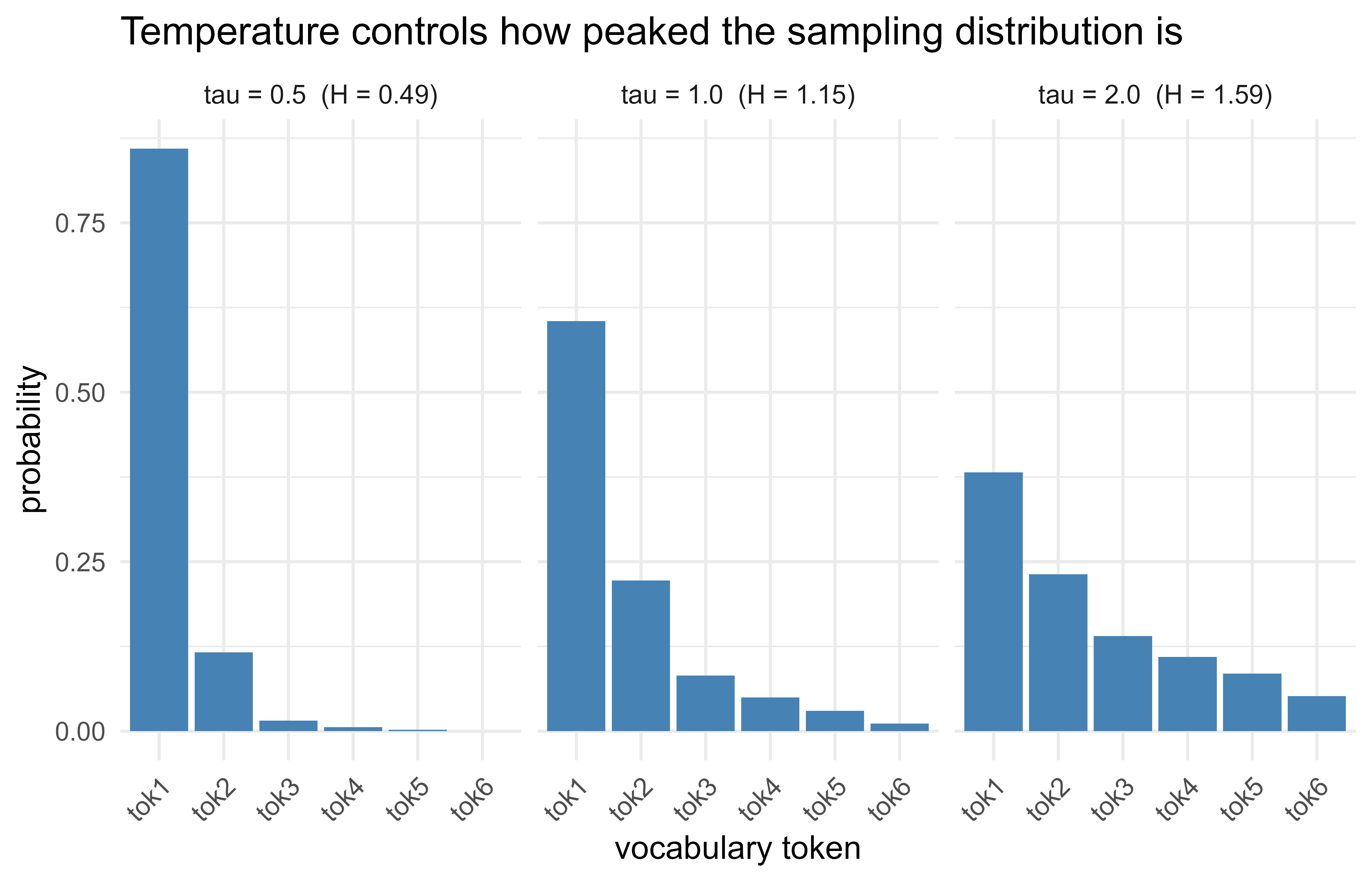
109.5.1 A figure: temperature reshapes the next-token distribution
To make the decoding math concrete, fix a single set of logits and plot the softmax distribution at several temperatures, with the entropy annotated. This is the mechanism behind the reliability/diversity trade-off. Figure Figure 109.1 shows how the same logits give a peaked distribution at low temperature and a flat one at high temperature.
Figure 109.1: Effect of temperature on the next-token distribution for a fixed set of logits. Low temperature concentrates mass on the top token (low entropy, near-deterministic); high temperature flattens the distribution (high entropy, diverse but less reliable).
109.5.2 A small simulation: temperature versus parse reliability
The argument that low temperature helps structured output can be simulated. Model a generator that, with probability \(q(\tau)\), emits schema-valid JSON and otherwise emits malformed output, where \(q\) decreases as \(\tau\) rises (hotter sampling wanders off-format more often). We estimate the valid-parse rate by Monte Carlo across temperatures.
Show code
set.seed(7)# Probability of a clean, schema-valid reply as a function of temperature.# Monotone decreasing: a stylized but realistic relationship.q_valid<-function(tau)plogis(3-1.6*tau)simulate_rate<-function(tau, n=4000){clean<-rbinom(n, 1, q_valid(tau))raw<-ifelse(clean==1,'{"reasoning": "ok", "label": "positive"}','Sure! label is positive')# off-format, no JSON objectvalid<-vapply(raw, function(r)process_reply(r, schema)$valid,logical(1))mean(valid)}taus<-c(0.0, 0.5, 1.0, 1.5, 2.0)rates<-sapply(taus, simulate_rate)data.frame(temperature =taus, valid_parse_rate =round(rates, 3))#> temperature valid_parse_rate#> 1 0.0 0.950#> 2 0.5 0.899#> 3 1.0 0.805#> 4 1.5 0.640#> 5 2.0 0.438
The estimated valid-parse rate falls as temperature rises, which is the empirical face of the entropy argument: hotter distributions put more mass on tokens that break the format. For a task you intend to parse, this is a direct reason to decode cold.
Note
The relationship \(q(\tau)\) here is stylized, chosen to illustrate the mechanism rather than measured from a specific model. The qualitative conclusion (cold decoding parses more reliably) is what holds in practice; the exact numbers will depend on the model and the task.
109.6 Practical guidance, pitfalls, and when to use it
Knowing when to reach for prompting, and when to put it down, is half the skill. Prompt engineering is the right first tool when the task is expressible in instructions, the base model is already competent at the underlying skill, you need a baseline fast, or labeled data is scarce. Classification, extraction, routing, reformatting, and summarization all fit this description. You should reach past it when prompting plateaus below your accuracy target on a held-out set (consider retrieval or fine-tuning), when the task needs private knowledge that is not in the prompt (retrieval), or when the latency and cost of long few-shot prompts start to dominate (distill into a smaller fine-tuned model).
A handful of concrete practices pay off repeatedly, and they follow directly from the ideas above:
Put the contract in the system prompt and the data in the user prompt. State the output schema explicitly, including the allowed values.
Order few-shot examples for coverage, including at least one example of each label and at least one hard or boundary case. Keep the example format byte-for-byte identical to what you ask for; the model copies the format it sees.
Always validate, never trust. Parse, validate against a schema, and have a defined action on failure (retry with a corrective message, lower temperature, or emit a default record). Log validation failures; they are your evaluation signal, and feed naturally into a broader evaluation harness (Chapter 113).
Decode cold for anything you parse. Set temperature near \(0\) and top-\(p\) modest. Save high temperature for genuinely open-ended generation.
Pin versions. Prompts, schemas, model name, and decoding parameters are all part of the artifact. A prompt that worked on one model version can drift on the next, so evaluate on a fixed test set when any of these change.
The same ideas, read backward, name the most common ways teams get burned. Watch for these pitfalls in particular:
Parsing without validating. Valid JSON with a wrong field value passes fromJSON and poisons everything downstream.
Putting chain-of-thought after the answer. Because generation is left to right, reasoning placed after the answer cannot inform it. Emit reasoning first, inside the JSON object.
Overstuffed prompts. Past a point, more examples cost tokens and latency without raising accuracy, and can dilute the instruction. Measure, do not assume more is better.
Hidden nondeterminism. Forgetting that temperature \(> 0\) makes outputs irreproducible, which makes bugs intermittent and evaluation noisy.
Tip
Treat the prompt, schema, model name, and decoding settings as one versioned artifact and keep a small fixed test set beside it. Then any change, including a silent model upgrade on the provider’s side, can be caught by rerunning the evaluation rather than by a user noticing broken output.
109.6.1 Swapping the stub for a real model
This is where the deterministic stub pays off. The demo isolates the model behind one function, model_stub(prompt, ...), so replacing it with a real client changes only that call; the template builder and the validator are unchanged. The chapter on calling LLM APIs from R (Chapter 108) covers the client side in depth. The snippet below sketches the shape of that call with a current R client. It is marked eval=FALSE because it needs the ellmer package and a live API key, neither of which is available in the book’s build environment, so it is shown for reference but not run.
Show code
# Conceptual: route the assembled prompt to a real model and reuse the same# validator. Requires a package not installed in this book's environment, so it# is shown but not run. The 'ellmer' package provides a tidy R interface.library(ellmer)chat<-chat_anthropic( system_prompt =prompt$system, model ="claude-3-5-sonnet-latest", api_args =list(temperature =0)# decode cold for parseable output)raw_reply<-chat$chat(prompt$user)# returns the model's textresult<-process_reply(raw_reply, schema)# same validator as aboveif(!result$valid){# Corrective retry: tell the model exactly what was wrong and ask again.fix_msg<-paste("Your reply was invalid:",paste(result$errors, collapse ="; "),"Return ONLY valid JSON matching the schema.")raw_reply<-chat$chat(fix_msg)result<-process_reply(raw_reply, schema)}
The discipline transfers directly to other interfaces. With OpenAI-style or Anthropic tool schemas you would pass the JSON schema in the request so the service constrains decoding, but you still run validate_against on the result, because syntactic validity does not guarantee your field constraints.
109.7 Further reading
Brown, T. B., et al. (2020). Language Models Are Few-Shot Learners (GPT-3). Advances in Neural Information Processing Systems.
Wei, J., Wang, X., Schuurmans, D., Bosma, M., Ichter, B., Xia, F., Chi, E., Le, Q., and Zhou, D. (2022). Chain-of-Thought Prompting Elicits Reasoning in Large Language Models. Advances in Neural Information Processing Systems.
Holtzman, A., Buys, J., Du, L., Forbes, M., and Choi, Y. (2020). The Curious Case of Neural Text Degeneration (nucleus sampling). International Conference on Learning Representations.
Kojima, T., Gu, S. S., Reid, M., Matsuo, Y., and Iwasawa, Y. (2022). Large Language Models Are Zero-Shot Reasoners. Advances in Neural Information Processing Systems.
Liu, P., Yuan, W., Fu, J., Jiang, Z., Hayashi, H., and Neubig, G. (2023). Pre-train, Prompt, and Predict: A Systematic Survey of Prompting Methods in Natural Language Processing. ACM Computing Surveys.
Ouyang, L., et al. (2022). Training Language Models to Follow Instructions with Human Feedback (InstructGPT). Advances in Neural Information Processing Systems.
We deliberately do not call a paid API. A small deterministic stub stands in for the model, which keeps the chapter fully reproducible and lets you see every moving part. The last section shows the one-line change that swaps the stub for a real client.↩︎
Instruction-tuned models are trained so that text marked as a system message is treated as higher-priority guidance than text in a user message. The roles are not magic, but the training makes them behave as if they were.↩︎
A logit is an unnormalized score, the raw output before it is turned into a probability. The vocabulary is the fixed set of tokens the model can emit, often tens of thousands of word pieces.↩︎
JSON, JavaScript Object Notation, is a simple text format for nested key-value data. A “schema” is a description of what a valid object looks like, much like a column specification for a data frame.↩︎
This is the mechanism behind “agents” and tool-using assistants, developed in Chapter 112. The model never runs code itself; it only proposes a structured call, and your program decides whether and how to honor it.↩︎
Source Code
# Prompt Engineering and Structured Output {#sec-prompt-engineering}```{r}#| include: falsesource("_common.R")```Most of this book studies models whose parameters you fit. With a pretrainedlarge language model (LLM) you usually do not fit parameters at all. You shapebehavior by what you put in the context window: instructions, examples, and aspecification of the output you want back. Prompt engineering is thediscipline of designing that input so the model produces useful, parseable,reliable results. Structured output is the part of that discipline thatforces the model to answer in a machine-readable format (typically JSON) so theresult can flow into the rest of a data pipeline.Here is the intuition before any formalism. Think of a pretrained LLM as a fixedfunction that takes a block of text in and produces a block of text out. Youcannot reach inside and retune it, but you can decide exactly what text goes in,and you can decide how adventurous the model is allowed to be when it writes theoutput. Those are the only two dials you have, and almost everything in thischapter is a careful use of one of them. The reward for using them well is large:a task that would normally need a labeled dataset and a training run can often besolved by writing a few paragraphs of instructions and reading back a small,well-shaped result.This chapter treats prompting as a design problem with measurable trade-offs,not folklore. We define the objects (system prompt, user prompt, few-shotexamples, tool schemas), give the probabilistic meaning of the decodingparameters that control randomness (temperature and top-$p$), and show whyasking for JSON and then validating it is the difference between a demo and aproduction component. By the end you will be able to read a prompt as a program,explain in probabilistic terms what temperature does to the output, and turn achatty text generator into something a downstream job can call like a typedfunction. The runnable demonstration is implemented in base R plus `glue`: aprompt-template function that assembles a few-shot prompt from a table ofexamples, plus a small JSON-schema validator that checks whether a model's(simulated) reply conforms to the contract you asked for.^[We deliberately donot call a paid API. A small deterministic stub stands in for the model, whichkeeps the chapter fully reproducible and lets you see every moving part. The lastsection shows the one-line change that swaps the stub for a real client.]::: {.callout-important title="Key idea"}With a frozen LLM you never change the model. You change itsinput (the prompt) and you change how you sample from its output (the decodingparameters). Hold on to that distinction and the rest of the chapter is justtwo levers.:::## Where this fits in a modern ML/AI workflowIn a classical supervised pipeline you collect labels, train a model, and serveit. With a capable instruction-tuned LLM you often skip training entirely for afirst version of a task: classification, extraction, summarization, routing, anddata cleaning can be done by describing the task in a prompt and reading backstructured fields. The prompt is the program.This matters for a data team in three concrete ways. The first is speed to abaseline: a zero-shot or few-shot prompt is a working baseline in minutes, beforeanyone labels a training set, and it tells you almost immediately whether thetask is even well posed. The second is that structured output acts as an APIcontract. If the model returns free text, a human has to read it; if it returnsJSON that matches a fixed schema, a downstream job can consume it like any otherservice. Validation is what turns a stochastic text generator into a typedfunction. The third is that prompting sits at the bottom of a clean fallbackladder. Prompting, few-shot prompting, retrieval (@sec-retrieval-augmented-generation),tool use (@sec-llm-agents), and fine-tuning arenot competitors but rungs you climb only when the cheaper rung fails itsevaluation. Prompt engineering is the rung you should exhaust first.::: {.callout-tip title="When to use this"}Start with a prompt whenever the task can be described inwords and the base model is already good at the underlying skill. Climb toretrieval or fine-tuning only after a held-out evaluation shows the prompt hasplateaued below your target. Cheaper rungs first, always.:::The mental model for the rest of the chapter: an LLM defines a conditionaldistribution over output tokens given the input tokens, $p_\theta(y \mid x)$with frozen parameters $\theta$. You do not change $\theta$. You change $x$ (theprompt) and you change how you *sample* from $p_\theta(\cdot \mid x)$ (thedecoding parameters). Everything below is one of those two levers.## The anatomy of a promptBefore we can shape a prompt, we need names for its parts. Modern chat modelsaccept a list of messages, each tagged with a role, and you control three ofthem. The system prompt holds persistent instructions that set the model'stask, tone, constraints, and output format; it is read once and conditionseverything after it, so this is where the contract belongs ("You are aclassifier. Return only JSON matching this schema."). The user prompt is thespecific request or input to act on, for example the one document you wantclassified. Assistant messages are the model's replies, and you can alsofabricate them to supply worked examples (few-shot), where each example is a userturn followed by the ideal assistant turn.::: {.callout-tip}The split between system and user prompts is the split between "rulesthat hold for every call" and "the one item this call is about." Putting theoutput schema in the system prompt and the data in the user prompt keeps thecontract stable while the input varies.:::Formally, the input $x$ is the concatenation of the rendered messages,$x = \texttt{render}(m_1, \dots, m_k)$, where each $m_i = (\text{role}_i,\text{content}_i)$. The model never sees roles as anything magical; they arespecial tokens in $x$.^[Instruction-tuned models are trained so that text markedas a system message is treated as higher-priority guidance than text in a usermessage. The roles are not magic, but the training makes them behave as if theywere.] The practical consequence is that the *order* and *labeling* of contentchanges the conditional distribution, which is why moving an instruction from theuser turn into the system turn can change behavior.### Zero-shot, few-shot, and chain-of-thoughtThree prompting patterns cover most applied use, and they differ only in whatextra content you place in $x$. Zero-shot prompting describes the task, givesthe input, and asks for the answer, with no examples at all; it works when thetask is common and the instruction is unambiguous. Few-shot promptingprepends $n$ solved examples $(u_1, a_1), \dots, (u_n, a_n)$ before the realinput $u^\*$, so the examples teach the format and the decision boundary bydemonstration. This is in-context learning: the model adapts its behaviorfrom examples in the prompt with no weight update (Brown et al., 2020).Chain-of-thought (CoT) prompting asks the model to produce intermediatereasoning steps before the final answer (Wei et al., 2022); for multi-stepproblems such as arithmetic, logic, or multi-hop questions this raises accuracy,because the intermediate tokens give the autoregressive model a scratchpad, andlater tokens condition on the reasoning it already wrote.::: {.callout-tip title="Intuition"}A model generates one token at a time, each conditioned oneverything before it. Letting it "think out loud" first means the final answeris generated in the presence of useful intermediate work, rather than beingguessed in a single leap. The scratchpad is the point.:::There is a real tension between CoT and structured output. Free-form reasoningis text, not JSON. The standard resolution is to keep the reasoning *inside* afield of the JSON object, for example a `"reasoning"` string emitted before the`"answer"` field, so you get the accuracy benefit and a parseable result. Theordering matters: because generation is left to right, the model must write thereasoning field first for it to actually inform the answer field.## Decoding parameters: the probabilistic viewWe have talked about changing the input $x$. The second lever is how you drawthe output from $p_\theta(\cdot \mid x)$, and it is controlled by a handful ofdecoding parameters. The intuition is simple: the model assigns a score toevery possible next word, and these parameters decide whether you always take thetop-scoring word or occasionally gamble on a lower-scoring one. Taking the topword every time is repeatable and safe; gambling adds variety at the cost ofreliability. The math below just makes "gamble how much" precise.At each step the model produces a vector of logits $z \in \mathbb{R}^{V}$over a vocabulary of size $V$.^[A logit is an unnormalized score, the raw outputbefore it is turned into a probability. The vocabulary is the fixed set of tokensthe model can emit, often tens of thousands of word pieces.] The next-tokendistribution is a softmax of those logits scaled by the temperature$\tau > 0$:$$p_\tau(v) = \frac{\exp(z_v / \tau)}{\sum_{u=1}^{V} \exp(z_u / \tau)}, \qquad v = 1, \dots, V.$$Temperature reshapes the same logits without retraining anything.- As $\tau \to 0^{+}$ the distribution concentrates on $\arg\max_v z_v$. Sampling becomes deterministic and equals greedy decoding.- At $\tau = 1$ you sample from the model's native distribution.- As $\tau$ grows the distribution flattens toward uniform, so rare tokens get more mass and output gets more diverse and less reliable.A useful way to quantify "how flat" the distribution is is the entropy$H(p_\tau) = -\sum_v p_\tau(v) \log p_\tau(v)$, which increases monotonicallywith $\tau$ from $0$ (a point mass) toward $\log V$ (uniform). You can readentropy here as a single number summarizing how undecided the model is at thisstep: low entropy means it is confident in one token, high entropy means manytokens look roughly equally good.Top-$p$ (nucleus) sampling truncates the tail before sampling (Holtzman etal., 2020). Sort tokens by probability and keep the smallest set$\mathcal{N}_p$ whose cumulative mass first reaches $p$:$$\mathcal{N}_p = \min \Big\{ \mathcal{S} : \sum_{v \in \mathcal{S}} p_\tau(v) \ge p \Big\},$$then renormalize over $\mathcal{N}_p$ and sample. Setting $p = 1$ disablestruncation; small $p$ removes the long tail of implausible tokens while stillallowing variety among the plausible ones. Top-$k$ is the same idea butkeeps a fixed count $k$ of highest-probability tokens regardless of their mass.The practical rule that follows from the math: for tasks with a single correctanswer (classification, extraction, anything you will parse), push $\tau$ toward$0$ so the output is near-deterministic and reproducible. For open-endedgeneration where you want variety (brainstorming, drafting), raise $\tau$ anduse top-$p$ around $0.9$ to cut the worst tail.::: {.callout-warning}Any temperature above $0$ makes the output irreproducible. Thesame prompt can give different answers on different runs, which turns bugs intointermittent ghosts and makes evaluation noisy. If you are going to parse theresult, decode cold.:::@tbl-prompt-engineering-decoding-knobs summarizes the levers. Read itas a quick-reference card: each row is one knob, what it controls, and whichdirection to turn it.| Parameter | Symbol | Range | Effect | When to lower | When to raise ||---|---|---|---|---|---|| Temperature | $\tau$ | $(0, \infty)$ | scales logits before softmax | parsing, classification, reproducibility | brainstorming, creative drafts || Top-$p$ (nucleus) | $p$ | $(0, 1]$ | keep smallest set reaching mass $p$ | factual or structured output | diverse generation || Top-$k$ | $k$ | $\{1, 2, \dots\}$ | keep $k$ highest-probability tokens | tighten output | widen candidate set || Max tokens || $\{1, 2, \dots\}$ | hard cap on output length | control cost and latency | long reasoning or documents || Stop sequences || strings | end generation on a marker | enforce clean boundaries | rarely |: Decoding parameters that control how output is sampled from the model, the quantity each one affects, and the direction to turn each knob for reliable parsing versus open-ended generation. {#tbl-prompt-engineering-decoding-knobs}## Structured output and JSON schemasSo far we have shaped the input and tuned the sampling. The last piece is shapingthe output, because a free-text answer is hard to consume programmatically. Thefix is to specify the exact shape of the output and ask the model to return onlythat. A JSON schema is a declarative description of an object: its fields,their types, which are required, and any value constraints (for example anenumeration of allowed labels).^[JSON, JavaScript Object Notation, is a simpletext format for nested key-value data. A "schema" is a description of what avalid object looks like, much like a column specification for a data frame.] Youput the schema (or a compact description of it) in the system prompt, and youvalidate the model's reply against it after generation.Two failure modes make validation non-optional. The first is format drift:the model wraps the JSON in prose ("Here is the result:") or in Markdown codefences, so you must extract the JSON substring before parsing. The second is aschema violation: the JSON parses cleanly but a required field is missing, atype is wrong, or a label is outside the allowed set, and only schema validationcatches this.::: {.callout-warning}Valid JSON is not the same as correct JSON. A reply can parseperfectly and still carry a label your pipeline has never heard of. Parsingwithout validating is the single most common way an LLM component silentlycorrupts the data downstream of it.:::The contract, then, is a short sequence: *parse, then validate, then act*. Ifvalidation fails you retry with a corrective message, lower the temperature, orfall back to a default record. Production LLM services also offer constraineddecoding that guarantees syntactically valid JSON, but valid JSON is not the sameas schema-conformant JSON, so you still validate the fields. The demo belowimplements parse and validate from scratch so the moving parts are visible.### Function and tool schemasTool use generalizes structured output. Instead of returning a final answer, themodel returns a structured call to a named function whose argument shape isitself a JSON schema you provide. The model picks the function and fills thearguments; your code executes it and feeds the result back.^[This is themechanism behind "agents" and tool-using assistants, developed in@sec-llm-agents. The model never runs codeitself; it only proposes a structured call, and your program decides whether andhow to honor it.] A weather assistantmight expose a `get_weather(location: string, unit: enum["C","F"])` tool; themodel emits `{"name": "get_weather", "arguments": {"location": "Paris", "unit":"C"}}`. From the model's side this is the same skill as structured output: emitJSON that matches a declared schema. The only new piece is that you, not themodel, decide what to do with the validated arguments.## Prompt templates: the runnable demoA prompt template is a string with named slots that you fill from data. Keepingtemplates as functions (rather than pasting strings) makes prompts versionable,testable, and consistent across thousands of calls. The demo builds a few-shotsentiment classifier prompt from a table of labeled examples, then validates a(simulated) model reply against a JSON schema. We do not call a paid API here; asmall deterministic stub stands in for the model so the chapter is fullyrunnable and reproducible. Swapping the stub for a real client is a one-linechange shown at the end.```{r pe-setup, eval=TRUE, message=FALSE}suppressPackageStartupMessages(library(glue))suppressPackageStartupMessages(library(jsonlite))set.seed(1301)# Few-shot examples: an input text and its gold label.examples <-data.frame(text =c("This product exceeded my expectations.","Worst purchase I have ever made.","It works, nothing special either way."),label =c("positive", "negative", "neutral"),stringsAsFactors =FALSE)# The allowed labels define the enum constraint in our schema.allowed_labels <-c("positive", "negative", "neutral")```The template function renders a system prompt that states the contract, a blockof few-shot examples, and the new input. Using `glue` keeps the slots explicit.```{r pe-template, eval=TRUE}render_examples <-function(ex) {# One example per shot: a user line then the ideal JSON assistant line. lines <-vapply(seq_len(nrow(ex)), function(i) { gold <-toJSON(list(reasoning ="stated explicitly in the text",label = ex$label[i]),auto_unbox =TRUE)glue("Input: {ex$text[i]}\nOutput: {gold}") }, character(1))paste(lines, collapse ="\n\n")}build_prompt <-function(new_text, ex, labels) { system_prompt <-glue("You are a sentiment classifier. Read the input text and return ONLY a ","JSON object with two fields: \"reasoning\" (a short string written first) ","and \"label\" (one of: {paste(labels, collapse = ', ')}). ","Do not add any text outside the JSON." ) shots <-render_examples(ex) user_prompt <-glue("Input: {new_text}\nOutput:")list(system =as.character(system_prompt),user =paste(shots, user_prompt, sep ="\n\n"))}prompt <-build_prompt("Absolutely fantastic, I love it.", examples, allowed_labels)cat(prompt$system, "\n\n---\n\n", prompt$user, sep ="")```Next, the JSON-schema validator. We define the schema as an R list and check aparsed object field by field: required presence, type, and (for `label`) theallowed enumeration. This is the same logic a production schema validatorapplies, written out so each check is visible.```{r pe-validate, eval=TRUE}# Schema: required fields, their JSON types, and optional enum constraints.schema <-list(reasoning =list(type ="string", required =TRUE),label =list(type ="string", required =TRUE, enum = allowed_labels))json_type <-function(x) {if (is.logical(x)) return("boolean")if (is.numeric(x)) return("number")if (is.character(x)) return("string")if (is.list(x)) return("object")"unknown"}extract_json <-function(txt) {# Strip code fences and surrounding prose: keep the first {...} block. m <-regmatches(txt, regexpr("\\{.*\\}", txt, perl =TRUE))if (length(m) ==0) NA_character_else m}validate_against <-function(obj, schema) { errs <-character(0)for (field innames(schema)) { spec <- schema[[field]]if (is.null(obj[[field]])) {if (isTRUE(spec$required)) errs <-c(errs, glue("missing required field '{field}'"))next }if (json_type(obj[[field]]) != spec$type) errs <-c(errs, glue("field '{field}' has type ","'{json_type(obj[[field]])}', expected '{spec$type}'"))if (!is.null(spec$enum) &&!(obj[[field]] %in% spec$enum)) errs <-c(errs, glue("field '{field}' value '{obj[[field]]}' ","not in allowed set")) }list(valid =length(errs) ==0, errors = errs)}# End to end: take raw model text, extract JSON, parse, validate.process_reply <-function(raw_text, schema) { js <-extract_json(raw_text)if (is.na(js)) return(list(valid =FALSE, errors ="no JSON found", obj =NULL)) obj <-tryCatch(fromJSON(js, simplifyVector =TRUE),error =function(e) NULL)if (is.null(obj)) return(list(valid =FALSE,errors ="JSON did not parse", obj =NULL)) res <-validate_against(obj, schema)c(res, list(obj = obj))}```Now a deterministic model stub. A real LLM is stochastic; here we mimic threerealistic reply styles so we can exercise the validator: a clean reply, a replywrapped in prose and a code fence, and a reply with an out-of-schema label.```{r pe-stub, eval=TRUE}model_stub <-function(prompt, style =c("clean", "fenced", "bad_label")) { style <-match.arg(style)switch(style,clean ='{"reasoning": "strong positive wording", "label": "positive"}',fenced =paste0("Here is the result:\n```json\n",'{"reasoning": "clearly enthusiastic", "label": "positive"}',"\n```"),bad_label ='{"reasoning": "seems good", "label": "happy"}' )}styles <-c("clean", "fenced", "bad_label")results <-lapply(styles, function(s) { raw <-model_stub(prompt, s)process_reply(raw, schema)})names(results) <- stylesfor (s in styles) { r <- results[[s]]cat(sprintf("[%s] valid = %s", s, r$valid))if (!r$valid) cat(sprintf(" (%s)", paste(r$errors, collapse ="; ")))cat("\n")}```The clean and fenced replies validate, because the extractor strips the fence andthe surrounding prose. The `bad_label` reply, by contrast, parses as JSON butfails the enum check, which is exactly the violation that silently corrupts apipeline if you parse without validating. This is the warning from earlier madeconcrete: the validator, not the parser, is what protects you.### A figure: temperature reshapes the next-token distributionTo make the decoding math concrete, fix a single set of logits and plot thesoftmax distribution at several temperatures, with the entropy annotated. This isthe mechanism behind the reliability/diversity trade-off. Figure@fig-prompt-engineering-temperature shows how the same logits give a peakeddistribution at low temperature and a flat one at high temperature.```{r fig-prompt-engineering-temperature, eval=TRUE, fig.cap="Effect of temperature on the next-token distribution for a fixed set of logits. Low temperature concentrates mass on the top token (low entropy, near-deterministic); high temperature flattens the distribution (high entropy, diverse but less reliable).", fig.width=7, fig.height=4.5}suppressPackageStartupMessages(library(ggplot2))logits <-c(3.0, 2.0, 1.0, 0.5, 0.0, -1.0)tokens <-factor(paste0("tok", seq_along(logits)),levels =paste0("tok", seq_along(logits)))temps <-c(0.5, 1.0, 2.0)softmax_t <-function(z, tau) { e <-exp(z / tau); e /sum(e)}entropy <-function(p) -sum(p *log(p))df <-do.call(rbind, lapply(temps, function(tau) { p <-softmax_t(logits, tau)data.frame(token = tokens, prob = p,panel =sprintf("tau = %.1f (H = %.2f)", tau, entropy(p)))}))ggplot(df, aes(token, prob)) +geom_col(fill ="steelblue") +facet_wrap(~ panel) +labs(x ="vocabulary token", y ="probability",title ="Temperature controls how peaked the sampling distribution is") +theme_minimal(base_size =12) +theme(axis.text.x =element_text(angle =45, hjust =1))```### A small simulation: temperature versus parse reliabilityThe argument that low temperature helps structured output can be simulated. Modela generator that, with probability $q(\tau)$, emits schema-valid JSON andotherwise emits malformed output, where $q$ decreases as $\tau$ rises (hottersampling wanders off-format more often). We estimate the valid-parse rate byMonte Carlo across temperatures.```{r pe-sim, eval=TRUE}set.seed(7)# Probability of a clean, schema-valid reply as a function of temperature.# Monotone decreasing: a stylized but realistic relationship.q_valid <-function(tau) plogis(3-1.6* tau)simulate_rate <-function(tau, n =4000) { clean <-rbinom(n, 1, q_valid(tau)) raw <-ifelse(clean ==1,'{"reasoning": "ok", "label": "positive"}','Sure! label is positive') # off-format, no JSON object valid <-vapply(raw, function(r) process_reply(r, schema)$valid,logical(1))mean(valid)}taus <-c(0.0, 0.5, 1.0, 1.5, 2.0)rates <-sapply(taus, simulate_rate)data.frame(temperature = taus, valid_parse_rate =round(rates, 3))```The estimated valid-parse rate falls as temperature rises, which is theempirical face of the entropy argument: hotter distributions put more mass ontokens that break the format. For a task you intend to parse, this is a directreason to decode cold.::: {.callout-note}The relationship $q(\tau)$ here is stylized, chosen to illustrate themechanism rather than measured from a specific model. The qualitativeconclusion (cold decoding parses more reliably) is what holds in practice; theexact numbers will depend on the model and the task.:::## Practical guidance, pitfalls, and when to use itKnowing when to reach for prompting, and when to put it down, is half the skill.Prompt engineering is the right first tool when the task is expressible ininstructions, the base model is already competent at the underlying skill, youneed a baseline fast, or labeled data is scarce. Classification, extraction,routing, reformatting, and summarization all fit this description. You shouldreach past it when prompting plateaus below your accuracy target on a held-outset (consider retrieval or fine-tuning), when the task needs private knowledgethat is not in the prompt (retrieval), or when the latency and cost of longfew-shot prompts start to dominate (distill into a smaller fine-tuned model).A handful of concrete practices pay off repeatedly, and they follow directly fromthe ideas above:- Put the contract in the system prompt and the data in the user prompt. State the output schema explicitly, including the allowed values.- Order few-shot examples for coverage, including at least one example of each label and at least one hard or boundary case. Keep the example format byte-for-byte identical to what you ask for; the model copies the format it sees.- Always validate, never trust. Parse, validate against a schema, and have a defined action on failure (retry with a corrective message, lower temperature, or emit a default record). Log validation failures; they are your evaluation signal, and feed naturally into a broader evaluation harness (@sec-evaluating-llms).- Decode cold for anything you parse. Set temperature near $0$ and top-$p$ modest. Save high temperature for genuinely open-ended generation.- Pin versions. Prompts, schemas, model name, and decoding parameters are all part of the artifact. A prompt that worked on one model version can drift on the next, so evaluate on a fixed test set when any of these change.The same ideas, read backward, name the most common ways teams get burned. Watchfor these pitfalls in particular:- Parsing without validating. Valid JSON with a wrong field value passes`fromJSON` and poisons everything downstream.- Putting chain-of-thought after the answer. Because generation is left to right, reasoning placed after the answer cannot inform it. Emit reasoning first, inside the JSON object.- Overstuffed prompts. Past a point, more examples cost tokens and latency without raising accuracy, and can dilute the instruction. Measure, do not assume more is better.- Hidden nondeterminism. Forgetting that temperature $> 0$ makes outputs irreproducible, which makes bugs intermittent and evaluation noisy.::: {.callout-tip}Treat the prompt, schema, model name, and decoding settings as oneversioned artifact and keep a small fixed test set beside it. Then any change,including a silent model upgrade on the provider's side, can be caught byrerunning the evaluation rather than by a user noticing broken output.:::### Swapping the stub for a real modelThis is where the deterministic stub pays off. The demo isolates the model behindone function, `model_stub(prompt, ...)`, so replacing it with a real clientchanges only that call; the template builder and the validator are unchanged. Thechapter on calling LLM APIs from R (@sec-llm-apis-r) covers the client side indepth. The snippet below sketches the shape of that call with a current R client. It ismarked `eval=FALSE` because it needs the `ellmer` package and a live API key,neither of which is available in the book's build environment, so it is shown forreference but not run.```{r pe-real-client, eval=FALSE}# Conceptual: route the assembled prompt to a real model and reuse the same# validator. Requires a package not installed in this book's environment, so it# is shown but not run. The 'ellmer' package provides a tidy R interface.library(ellmer)chat <-chat_anthropic(system_prompt = prompt$system,model ="claude-3-5-sonnet-latest",api_args =list(temperature =0) # decode cold for parseable output)raw_reply <- chat$chat(prompt$user) # returns the model's textresult <-process_reply(raw_reply, schema) # same validator as aboveif (!result$valid) {# Corrective retry: tell the model exactly what was wrong and ask again. fix_msg <-paste("Your reply was invalid:",paste(result$errors, collapse ="; "),"Return ONLY valid JSON matching the schema.") raw_reply <- chat$chat(fix_msg) result <-process_reply(raw_reply, schema)}```The discipline transfers directly to other interfaces. With OpenAI-style orAnthropic tool schemas you would pass the JSON schema in the request so theservice constrains decoding, but you still run `validate_against` on the result,because syntactic validity does not guarantee your field constraints.## Further reading- Brown, T. B., et al. (2020). Language Models Are Few-Shot Learners (GPT-3). *Advances in Neural Information Processing Systems*.- Wei, J., Wang, X., Schuurmans, D., Bosma, M., Ichter, B., Xia, F., Chi, E., Le, Q., and Zhou, D. (2022). Chain-of-Thought Prompting Elicits Reasoning in Large Language Models. *Advances in Neural Information Processing Systems*.- Holtzman, A., Buys, J., Du, L., Forbes, M., and Choi, Y. (2020). The Curious Case of Neural Text Degeneration (nucleus sampling). *International Conference on Learning Representations*.- Kojima, T., Gu, S. S., Reid, M., Matsuo, Y., and Iwasawa, Y. (2022). Large Language Models Are Zero-Shot Reasoners. *Advances in Neural Information Processing Systems*.- Liu, P., Yuan, W., Fu, J., Jiang, Z., Hayashi, H., and Neubig, G. (2023). Pre-train, Prompt, and Predict: A Systematic Survey of Prompting Methods in Natural Language Processing. *ACM Computing Surveys*.- Ouyang, L., et al. (2022). Training Language Models to Follow Instructions with Human Feedback (InstructGPT). *Advances in Neural Information Processing Systems*.