Suppose you have a million customer support tickets and a new one arrives reading “I can’t log in.” You want the handful of past tickets that mean the same thing, even when they used different words (“forgot my password,” “account locked out”). Keyword matching fails here: the words barely overlap. What you really want is to measure closeness in meaning, and that turns out to be possible once you give every ticket a position in space.
Modern machine learning systems represent text, images, audio, and other unstructured inputs as fixed-length numeric vectors called embeddings. The trick is that the vectors are arranged so that things with similar meaning sit close together. Once an object lives in a vector space, “find things like this one” stops being a vague linguistic question and becomes a concrete geometry problem: search for the vectors closest to a query vector.
Intuition
Think of an embedding as a coordinate on a map of meaning. Two cities that are close on a map are easy to travel between; two sentences that are close in embedding space are similar in meaning. Search becomes “which points are nearest this one,” exactly like finding the closest town.
This chapter covers how embeddings are produced, how similarity is measured, how to retrieve nearest neighbors quickly at scale, and the engineering tradeoffs that vector databases force you to make. By the end you will be able to compute similarities by hand in base R, run exact nearest-neighbor search, reason about the approximate indexes (HNSW and IVF) that power production systems, and recognize the failure modes that quietly break retrieval pipelines. The mathematics is light (mostly inner products and distances); the payoff is understanding the engine behind semantic search and retrieval-augmented generation.
110.1 Intuition and Where This Fits
An embedding is a learned map \(\phi: \mathcal{X} \to \mathbb{R}^d\) from raw objects (a sentence, a product description, an image) to a \(d\)-dimensional vector.1 The map is trained so that semantically similar objects land near each other and dissimilar objects land far apart. A typical text embedding model produces \(d\) between 384 and 3072.
Key idea
The intelligence lives in the encoder that produces the vectors. The search machinery in this chapter is “just” geometry. Once meaning has been baked into coordinates, finding similar items is a matter of measuring distances, which is fast and well understood.
Embeddings sit between raw data and downstream tasks in many pipelines. The most common uses are the following.
Retrieval augmented generation (RAG): a user question is embedded, the closest document chunks are retrieved by vector search, and those chunks are passed to a language model as context. This is the foundation of the retrieval-augmented generation chapter (Chapter 111).
Semantic search: rank documents by meaning rather than keyword overlap.
Recommendation: represent users and items in a shared space and recommend nearby items, as developed in the recommender systems chapter (Chapter 89).
Deduplication and clustering: near-duplicate detection and grouping by proximity (Chapter 23).
Classification features: embeddings are dense features for a simple downstream model such as logistic regression or gradient boosting (Chapter 12).
The reason this pattern is so common comes down to economics: training a good encoder is expensive and done once, but using it is cheap. You embed your corpus a single time, store the vectors, and answer queries with fast geometric lookups. The retrieval step is the part that has to scale to millions or billions of vectors, which is what most of this chapter is about.
When to use this
Reach for embeddings whenever “similar in meaning” matters more than “shares exact words,” when you need to compare items across modalities (text against images), or when you want dense numeric features for a classifier from inputs that have no natural numeric form. If exact-match or keyword lookup already solves your problem, a plain index is simpler and faster.
With that motivation in place, the rest of the chapter works from the bottom up: first how to measure closeness between two vectors, then how to find the closest vectors in a corpus, and finally how to do that search quickly when the corpus is huge.
110.2 Similarity and Distance
Before we can search for “near” vectors we have to say what “near” means. Let \(u, v \in \mathbb{R}^d\). The two measures that dominate embedding search are Euclidean distance and cosine similarity.
The Euclidean (L2) distance is \[
d_2(u, v) = \|u - v\|_2 = \sqrt{\sum_{j=1}^d (u_j - v_j)^2}.
\]
The cosine similarity is the cosine of the angle between the vectors, \[
\cos(u, v) = \frac{u^\top v}{\|u\|_2 \, \|v\|_2} = \frac{\sum_{j=1}^d u_j v_j}{\sqrt{\sum_j u_j^2}\,\sqrt{\sum_j v_j^2}},
\] which lies in \([-1, 1]\). A value near \(1\) means the vectors point in nearly the same direction, \(0\) means orthogonal, and \(-1\) means opposite. Cosine similarity ignores vector magnitude and looks only at direction, which is usually what you want for text: a long document and a short one about the same topic should still be judged similar.
Note
The contrast between the two measures is exactly the contrast between length and direction. Euclidean distance asks “how far apart are the tips of the arrows,” so it is sensitive to magnitude. Cosine similarity asks “do the arrows point the same way,” ignoring how long they are. For embeddings, direction carries the meaning and magnitude is often an artifact of input length, so cosine is the usual default.
110.2.1 The Connection Between Cosine and Euclidean Distance
These two measures are not independent. If you normalize every vector to unit length, \(\tilde{u} = u / \|u\|_2\), then \[
d_2(\tilde{u}, \tilde{v})^2 = \|\tilde u\|_2^2 + \|\tilde v\|_2^2 - 2\,\tilde u^\top \tilde v = 1 + 1 - 2\cos(u, v) = 2\bigl(1 - \cos(u, v)\bigr).
\] So on unit vectors, ranking by smallest Euclidean distance gives exactly the same order as ranking by largest cosine similarity. This is why most vector databases tell you to normalize your embeddings and then use either metric: the nearest neighbor set is identical. It also lets a library that only implements L2 search serve cosine queries after a one-time normalization.
Tip
The equation \(d_2(\tilde u, \tilde v)^2 = 2(1 - \cos(u,v))\) is worth committing to memory. It is the bridge that lets you move freely between the two worlds, and several code chunks below use it to convert an L2 distance the library reports back into the cosine similarity you actually wanted to read.
The related cosine distance is defined as \(1 - \cos(u, v)\), which is what many libraries report. Note it is not a true metric (it violates the triangle inequality), so be careful when an algorithm assumes metric properties.2
110.2.2 Exact k-Nearest-Neighbor Retrieval
Given a query \(q\) and a corpus \(\{v_1, \dots, v_n\}\), exact \(k\)-nearest-neighbor (kNN) retrieval returns the \(k\) indices with the largest \(\cos(q, v_i)\) (or smallest distance). The brute-force cost is \(O(nd)\) per query: you score every vector. That is fine for thousands of vectors but becomes the bottleneck at millions, which motivates approximate methods later in the chapter.
Warning
“Exact” here means the result is the true mathematical nearest neighbor, not that the answer is correct in any deeper sense. If the embeddings themselves are poor, exact search just retrieves the wrong things very precisely. Quality starts with the encoder; search only preserves whatever quality the vectors already have.
110.3 A Runnable Base R Demonstration
Everything so far has been definitions. The fastest way to make them concrete is to build a tiny corpus by hand and watch the geometry do its job. We construct toy embeddings so the structure is transparent, compute a cosine similarity matrix, run exact kNN retrieval, and draw a heatmap. This chunk uses only base R and runs as written.
Show code
set.seed(42)# Three latent "topics", each a random direction in R^d.d<-16n_topics<-3topic_dirs<-matrix(rnorm(n_topics*d), nrow =n_topics)# Generate documents: each doc picks a topic, then adds noise around# that topic's direction. This mimics what a real encoder does, namely# place semantically related items near a common direction.docs_per_topic<-5labels<-rep(seq_len(n_topics), each =docs_per_topic)doc_names<-paste0("T", labels, "_", ave(labels, labels, FUN =seq_along))noise<-0.6emb<-t(sapply(labels, function(k)topic_dirs[k, ]+rnorm(d, sd =noise)))rownames(emb)<-doc_names# L2-normalize every embedding to unit length.normalize_rows<-function(X)X/sqrt(rowSums(X^2))emb_n<-normalize_rows(emb)# On unit vectors, the full cosine similarity matrix is just the# inner-product (Gram) matrix.cos_sim<-emb_n%*%t(emb_n)# Exact kNN retrieval for a single query embedding.knn_search<-function(query, corpus_unit, k=3){q<-query/sqrt(sum(query^2))sims<-as.numeric(corpus_unit%*%q)ord<-order(sims, decreasing =TRUE)[seq_len(k)]data.frame(doc =rownames(corpus_unit)[ord], cosine =round(sims[ord], 3))}# Use document T2_1 as the query and retrieve its 4 nearest neighbors.query_vec<-emb["T2_1", ]cat("Query = T2_1; top matches (the query itself ranks first):\n")#> Query = T2_1; top matches (the query itself ranks first):print(knn_search(query_vec, emb_n, k =4))#> doc cosine#> 1 T2_1 1.000#> 2 T2_5 0.797#> 3 T2_4 0.781#> 4 T2_2 0.737# Heatmap of the cosine similarity matrix.ord<-order(labels)M<-cos_sim[ord, ord]op<-par(mar =c(5, 5, 3, 2))image( x =seq_len(nrow(M)), y =seq_len(ncol(M)), z =M, col =hcl.colors(32, "YlOrRd", rev =TRUE), axes =FALSE, xlab ="", ylab ="", main ="Cosine similarity between toy embeddings")axis(1, at =seq_len(nrow(M)), labels =rownames(M), las =2, cex.axis =0.7)axis(2, at =seq_len(ncol(M)), labels =colnames(M), las =2, cex.axis =0.7)box()par(op)
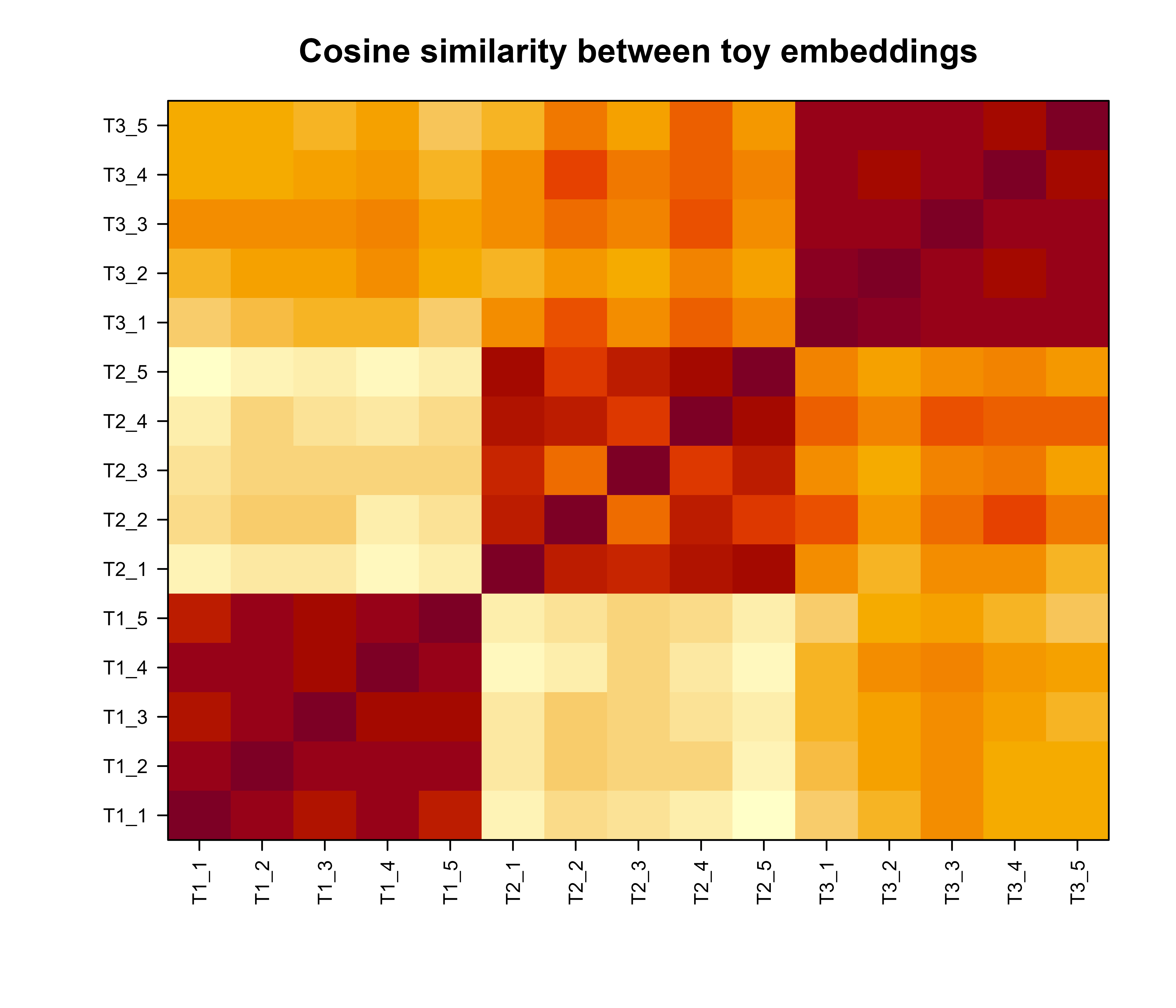
Figure 110.1: Cosine similarity heatmap of toy document embeddings drawn with base R. Documents from the same topic cluster form bright blocks along the diagonal.
Figure 110.1 shows the result. The bright square blocks along the diagonal are the within-topic similarities, and the dim off-diagonal regions are cross-topic pairs. The kNN query correctly returns the other documents from topic 2 as the closest matches. This is the entire mechanism behind semantic search, just at toy scale.
110.3.1 A ggplot2 Version of the Heatmap
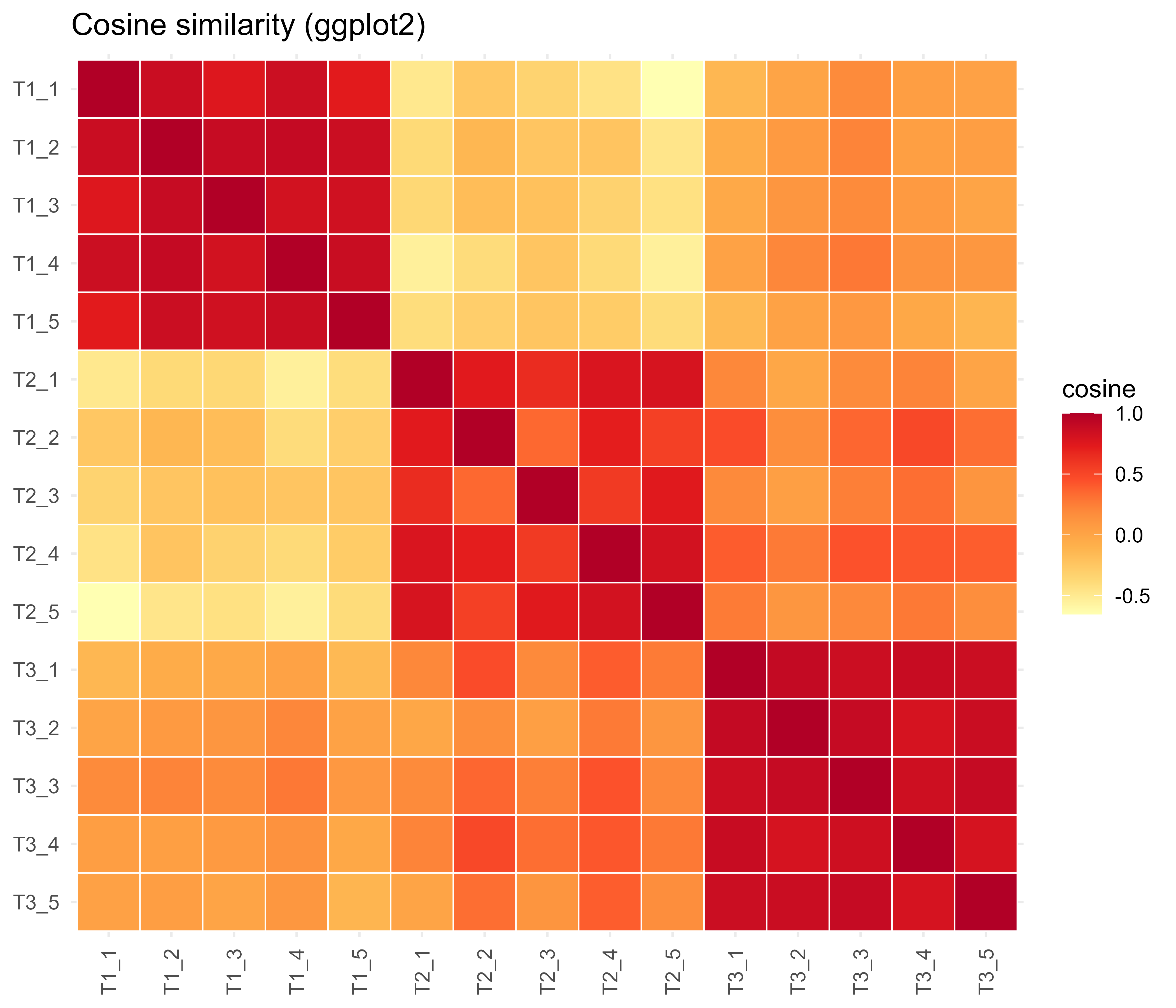
If you prefer the tidyverse, the same matrix is easy to plot with ggplot2, as Figure 110.2 shows. This chunk also runs as written.
Figure 110.2: The same cosine similarity matrix rendered with ggplot2 geom_tile, confirming the block structure seen in the base R version.
110.3.2 Exact kNN With an Installed Package
The FNN package (a recommended package that ships with R) computes exact nearest neighbors efficiently with a k-d tree. On unit-normalized vectors, L2 nearest neighbors equal cosine nearest neighbors, as derived above. This chunk runs as written.
Show code
library(FNN)# Query: the first document. get.knnx returns neighbors in the corpus# for each query row, using Euclidean distance.res<-get.knnx(data =emb_n, query =emb_n["T2_1", , drop =FALSE], k =4)neighbors<-rownames(emb_n)[res$nn.index[1, ]]# Convert L2 distance on unit vectors back to cosine: cos = 1 - dist^2 / 2.cosines<-1-res$nn.dist[1, ]^2/2data.frame(doc =neighbors, cosine =round(cosines, 3))#> doc cosine#> 1 T2_1 1.000#> 2 T2_5 0.797#> 3 T2_4 0.781#> 4 T2_2 0.737
The neighbor order matches the brute-force cosine search, confirming the equivalence. For a few thousand vectors this exact approach is all you need.
110.4 Approximate Nearest Neighbors
Exact search costs \(O(nd)\) per query. When \(n\) reaches tens of millions, that is too slow for interactive use. Approximate nearest neighbor (ANN) indexes trade a small, controllable loss in accuracy for large speedups, often returning 95 to 99 percent of the true neighbors in a fraction of the time. Accuracy is measured by recall@k: of the true top-\(k\) neighbors, what fraction did the index return.3
Intuition
Exact search reads every page of the book to answer a question. ANN is like using the index and the table of contents: you skip almost all the pages and accept a tiny chance of missing the one paragraph you wanted, in exchange for an answer that arrives in milliseconds.
Two index families dominate production systems. They take opposite routes to the same goal of avoiding a full scan: one navigates a graph of neighbors, the other narrows the search to a few clusters.
110.4.1 HNSW (Hierarchical Navigable Small World)
HNSW builds a multi-layer proximity graph. Each vector is a node connected to a bounded number of nearby vectors. Upper layers are sparse “express lanes” with long-range links; lower layers are dense and local. A search starts at an entry point in the top layer and greedily walks toward the query, descending layers until it reaches the bottom, where it does a fine-grained local search.
Intuition
HNSW works like an airline network. The top layer is a few hub airports with long-haul routes that cover huge distances in one hop; the bottom layer is the dense web of regional flights. To reach a small town you fly hub-to-hub first to get into the right region, then take short hops to the exact destination. That is why search is fast even with millions of nodes: most of the distance is covered by a handful of long edges.
The key parameters are the following.
\(M\): the number of neighbors stored per node. Larger \(M\) improves recall and increases memory and build time.
efConstruction: the size of the candidate list while building. Larger values build a higher-quality graph more slowly.
efSearch (sometimes ef): the size of the candidate list during a query. This is the main runtime knob, trading speed for recall without rebuilding the index.
Search time is roughly \(O(\log n)\) in practice, which is why HNSW dominates latency-sensitive workloads. The cost is memory: the graph edges add overhead on top of the raw vectors.
110.4.2 IVF (Inverted File Index)
IVF first runs k-means to partition the space into nlist clusters, each with a centroid. Every vector is assigned to its nearest centroid’s list. At query time you score the query against the centroids, pick the nprobe closest clusters, and search only the vectors in those lists. You scan a fraction \(\approx \text{nprobe} / \text{nlist}\) of the corpus instead of all of it.
Intuition
IVF is like a library organized into sections. Instead of walking every shelf, you decide your book is probably in the “history” and “biography” sections and search only those. nprobe is how many sections you are willing to browse; checking more raises your chance of finding the book but takes longer. The risk, as with a real library, is that the book was misshelved one section over.
The parameters are the following.
nlist: number of clusters (partitions). A common heuristic is \(\text{nlist} \approx \sqrt{n}\).
nprobe: number of clusters searched per query. Higher means better recall and slower queries. This is tunable at query time.
IVF pairs naturally with product quantization (PQ), which compresses each vector into a short code so billions of vectors fit in memory. PQ splits the \(d\) dimensions into \(m\) subvectors and replaces each with the index of its nearest centroid in a small per-subspace codebook, giving large compression at the cost of some precision.4 The combination IVF-PQ is the standard recipe for very large corpora.
Warning
PQ stores a lossy approximation of each vector, so the distances it computes are approximate even before any clustering shortcut. This is fine for a first-pass candidate list but a poor choice when you need precise scores. The standard fix is to re-rank the PQ candidates against the full vectors, a pattern we return to under practical guidance.
110.4.3 Comparison of Index Types
Table 110.1 summarizes the tradeoffs. Read it as a decision aid: pick the row whose “best for” column matches your corpus size and memory budget.
Table 110.1: Tradeoffs among common vector index types.
Index
Query speed
Recall
Memory
Build cost
Best for
Flat (exact)
Slow
100%
Full vectors
None
< ~100k vectors, exactness
HNSW
Very fast
High, tunable
Full vectors + graph
High
Low-latency, moderate memory
IVF-Flat
Fast
High, tunable
Full vectors + lists
Medium (k-means)
Large corpora, ample RAM
IVF-PQ
Fast
Medium, tunable
Compressed (small)
Medium (k-means + codebooks)
Very large corpora, tight RAM
110.5 ANN in Practice (Library Code)
The libraries that implement these indexes (FAISS, hnswlib, Annoy, ScaNN) are Python or C++ and are not in this book’s installed R set, so the chunks below are marked eval=FALSE. They are correct, idiomatic code a reader can run after installing the relevant tools.
Note
The pattern in every chunk below is the same three steps: build (or train) an index, add your vectors, then query. Once you recognize that skeleton, switching between hnswlib, FAISS, and a database is mostly a matter of renaming methods and translating parameters, not learning a new mental model.
110.5.1 hnswlib via reticulate
Show code
# Requires: pip install hnswlib, and the R 'reticulate' package.library(reticulate)hnswlib<-import("hnswlib")np<-import("numpy")# Suppose 'emb_n' is an n x d matrix of unit-normalized embeddings.n<-nrow(emb_n); d<-ncol(emb_n)data_py<-np$asarray(emb_n, dtype ="float32")# 'cosine' space; on unit vectors this equals inner-product / L2 ordering.index<-hnswlib$Index(space ="cosine", dim =as.integer(d))index$init_index(max_elements =as.integer(n), ef_construction =200L, M =16L)index$add_items(data_py, ids =np$arange(n))# efSearch is the main recall/speed knob; raise it for higher recall.index$set_ef(50L)query<-np$asarray(emb_n[1, , drop =FALSE], dtype ="float32")res<-index$knn_query(query, k =5L)labels<-res[[1]]# neighbor ids (0-based)dists<-res[[2]]# cosine distances = 1 - cosine similarity
110.5.2 FAISS IVF-PQ via reticulate
Show code
# Requires: pip install faiss-cpu, and the R 'reticulate' package.library(reticulate)faiss<-import("faiss")np<-import("numpy")d<-ncol(emb_n)xb<-np$asarray(emb_n, dtype ="float32")nlist<-100L# number of Voronoi cells (clusters)m<-8L# number of PQ subquantizers; must divide dnbits<-8L# bits per subquantizer codequantizer<-faiss$IndexFlatIP(d)# inner product for unit vectorsindex<-faiss$IndexIVFPQ(quantizer, d, nlist, m, nbits)index$train(xb)# k-means + codebook trainingindex$add(xb)index$nprobe<-10L# clusters searched per query; raise for recallxq<-np$asarray(emb_n[1, , drop =FALSE], dtype ="float32")res<-index$search(xq, 5L)distances<-res[[1]]indices<-res[[2]]
110.5.3 Producing Real Embeddings With keras
So far the vectors have been synthetic. To go beyond toy vectors you need an encoder, the learned map \(\phi\) from the start of the chapter made real. Below is the shape of producing sentence embeddings with a TensorFlow Hub universal sentence encoder loaded through keras/tensorflow. Per the book’s policy, keras and Python interop chunks are eval=FALSE.
Show code
# Requires a working keras/tensorflow install plus tensorflow_hub in Python.library(tensorflow)hub<-reticulate::import("tensorflow_hub")encoder<-hub$load("https://tfhub.dev/google/universal-sentence-encoder/4")docs<-c("How do I reset my password?","Steps to recover a forgotten login.","What is the refund policy?")emb_tensor<-encoder(docs)# shape: (3, 512)emb_real<-as.matrix(emb_tensor$numpy())# Normalize, then store in any vector index from the chunks above.emb_real<-emb_real/sqrt(rowSums(emb_real^2))
110.5.4 Storing Vectors in a Vector Database
In production the index and metadata live in a vector database (for example pgvector inside PostgreSQL, Qdrant, Weaviate, or Milvus). With pgvector the search is plain SQL using the cosine distance operator <=>. This needs DBI/RPostgres, which are not in the installed set, so it is eval=FALSE.
Show code
# Requires: PostgreSQL with the 'vector' extension, plus DBI + RPostgres.library(DBI)con<-dbConnect(RPostgres::Postgres(), dbname ="rag")dbExecute(con, "CREATE EXTENSION IF NOT EXISTS vector;")dbExecute(con, " CREATE TABLE IF NOT EXISTS chunks ( id bigserial PRIMARY KEY, body text, embedding vector(512) );")# An HNSW index for fast cosine search at scale.dbExecute(con, " CREATE INDEX IF NOT EXISTS chunks_hnsw ON chunks USING hnsw (embedding vector_cosine_ops) WITH (m = 16, ef_construction = 200);")# Retrieve the 5 chunks most similar to a query embedding 'q'# (q passed as a parameter formatted like '[0.1, 0.2, ...]').res<-dbGetQuery(con, " SELECT id, body, 1 - (embedding <=> $1) AS cosine_sim FROM chunks ORDER BY embedding <=> $1 LIMIT 5;", params =list(q_literal))dbDisconnect(con)
110.6 Practical Guidance and Pitfalls
The geometry is the easy part. Most retrieval systems that disappoint in production fail not because the math is wrong but because of mismatches and misconfigurations around the edges. The guidance below collects the failure modes that recur most often, roughly in the order you are likely to hit them.
Normalize, then decide the metric. Unit-normalize embeddings unless you have a specific reason not to. After normalization, cosine and L2 give identical rankings, and most models are trained with cosine objectives anyway. Mixing normalized and unnormalized vectors in one index silently corrupts results.
Match the query and document encoders. Embed the query with the same model (and the same normalization) used for the corpus. A common production bug is upgrading the document encoder but leaving the query path on the old model, which destroys recall.
Tune efSearch / nprobe against measured recall, not by guessing. Build a small ground-truth set with exact (Flat) search, then raise the runtime knob until recall@k crosses your target (say 0.95). These knobs change recall and latency at query time without rebuilding, so tune them last.
Watch dimensionality and storage. Raw float32 storage is \(4 \times n \times d\) bytes. Ten million vectors at \(d = 768\) is about 30 GB before any index overhead. If that does not fit in RAM, move to IVF-PQ or another quantized index rather than spilling to disk.
Chunk size matters in RAG. Embedding an entire long document into one vector blurs distinct topics together. Split into overlapping chunks of a few hundred tokens so each vector captures one coherent idea, and store enough metadata to reassemble context.
ANN is approximate by definition. Do not use an HNSW or IVF result where exactness is required (for example, exact deduplication or a legal lookup). Use Flat search, or re-rank the ANN candidates with exact scoring.
Re-ranking helps quality. A standard pattern is to retrieve a generous candidate set (say top 100) with a fast bi-encoder ANN search, then re-score the candidates with a slower, more accurate cross-encoder and keep the top 10. This recovers much of the quality lost to approximation and to the bi-encoder bottleneck.
Filtering interacts badly with ANN. Combining a metadata filter (for example, “only documents from 2025”) with ANN can leave a graph or cluster nearly empty of matching vectors, hurting recall. Prefer databases that support filtered vector search natively rather than filtering after retrieval.
Tip
If you take away one habit from this section, make it this: build a small exact ground-truth set and measure recall@k before you trust an ANN index. Almost every pitfall above shows up as a quiet drop in recall, and you cannot fix a number you never measured.
110.6.1 When to Use What
To close, here is a quick decision guide that maps the common situations onto the index choices developed above.
Fewer than roughly 100k vectors, or exactness required: use Flat / exact kNN. The FNN approach above is enough.
Low-latency interactive search with vectors that fit in RAM: use HNSW.
Very large corpora that strain memory: use IVF-PQ or another quantized index, and accept lower recall in exchange for footprint.
Want SQL, transactions, and metadata alongside vectors: use a vector-capable database such as pgvector.
The thread running through all of these choices is the same tradeoff triangle: speed, accuracy, and memory. You can usually have any two cheaply, and the index families exist precisely to let you pick which one to spend on. Start exact, measure, and add approximation only when the corpus forces you to.
110.7 Further Reading
Mikolov, T., Sutskever, I., Chen, K., Corrado, G., and Dean, J. (2013). Distributed representations of words and phrases and their compositionality. Introduces word2vec.
Pennington, J., Socher, R., and Manning, C. (2014). GloVe: Global vectors for word representation.
Devlin, J., Chang, M.-W., Lee, K., and Toutanova, K. (2019). BERT: Pre-training of deep bidirectional transformers for language understanding.
Reimers, N., and Gurevych, I. (2019). Sentence-BERT: Sentence embeddings using Siamese BERT-networks.
Johnson, J., Douze, M., and Jegou, H. (2019). Billion-scale similarity search with GPUs. The FAISS paper.
Malkov, Y. A., and Yashunin, D. A. (2018). Efficient and robust approximate nearest neighbor search using hierarchical navigable small world graphs. The HNSW paper.
Jegou, H., Douze, M., and Schmid, C. (2011). Product quantization for nearest neighbor search.
Lewis, P., et al. (2020). Retrieval-augmented generation for knowledge-intensive NLP tasks.
The word “learned” is doing real work here. The map \(\phi\) is not hand-designed; it is the output of training a neural network (often a transformer, Chapter 38) on a large corpus, so that the geometry of the output space reflects patterns the model picked up from data.↩︎
A true metric must satisfy the triangle inequality \(d(a,c) \le d(a,b) + d(b,c)\). Cosine distance does not, which matters for methods like metric trees that prune the search using that inequality. The squared Euclidean distance on normalized vectors, by contrast, behaves itself, another reason to normalize and then think in L2 terms.↩︎
For example, if the true 10 nearest neighbors are a set \(T\) and the index returns a set \(R\) of size 10, recall@10 is \(|T \cap R| / 10\). A recall of 0.97 means the index missed, on average, about one of every 33 true neighbors. Whether that matters depends entirely on the application.↩︎
As a rough sense of scale: a 768-dimensional float32 vector is about 3 KB. Split into \(m = 8\) subvectors each coded with 8 bits, it shrinks to 8 bytes, a roughly 400-fold reduction. You no longer store the vector itself, only the codebook indices, which is why a billion vectors can fit in memory at all.↩︎
Source Code
# Embeddings and Vector Search {#sec-embeddings-vector-search}```{r}#| include: falsesource("_common.R")```Suppose you have a million customer support tickets and a new one arrives reading "I can't log in." You want the handful of past tickets that mean the same thing, even when they used different words ("forgot my password," "account locked out"). Keyword matching fails here: the words barely overlap. What you really want is to measure closeness in *meaning*, and that turns out to be possible once you give every ticket a position in space.Modern machine learning systems represent text, images, audio, and other unstructured inputs as fixed-length numeric vectors called embeddings. The trick is that the vectors are arranged so that things with similar meaning sit close together. Once an object lives in a vector space, "find things like this one" stops being a vague linguistic question and becomes a concrete geometry problem: search for the vectors closest to a query vector.::: {.callout-tip title="Intuition"}Think of an embedding as a coordinate on a map of meaning. Two cities that are close on a map are easy to travel between; two sentences that are close in embedding space are similar in meaning. Search becomes "which points are nearest this one," exactly like finding the closest town.:::This chapter covers how embeddings are produced, how similarity is measured, how to retrieve nearest neighbors quickly at scale, and the engineering tradeoffs that vector databases force you to make. By the end you will be able to compute similarities by hand in base R, run exact nearest-neighbor search, reason about the approximate indexes (HNSW and IVF) that power production systems, and recognize the failure modes that quietly break retrieval pipelines. The mathematics is light (mostly inner products and distances); the payoff is understanding the engine behind semantic search and retrieval-augmented generation.## Intuition and Where This FitsAn embedding is a learned map $\phi: \mathcal{X} \to \mathbb{R}^d$ from raw objects (a sentence, a product description, an image) to a $d$-dimensional vector.^[The word "learned" is doing real work here. The map $\phi$ is not hand-designed; it is the output of training a neural network (often a transformer, @sec-transformers) on a large corpus, so that the geometry of the output space reflects patterns the model picked up from data.] The map is trained so that semantically similar objects land near each other and dissimilar objects land far apart. A typical text embedding model produces $d$ between 384 and 3072.::: {.callout-important title="Key idea"}The intelligence lives in the encoder that produces the vectors. The search machinery in this chapter is "just" geometry. Once meaning has been baked into coordinates, finding similar items is a matter of measuring distances, which is fast and well understood.:::Embeddings sit between raw data and downstream tasks in many pipelines. The most common uses are the following.- Retrieval augmented generation (RAG): a user question is embedded, the closest document chunks are retrieved by vector search, and those chunks are passed to a language model as context. This is the foundation of the retrieval-augmented generation chapter (@sec-retrieval-augmented-generation).- Semantic search: rank documents by meaning rather than keyword overlap.- Recommendation: represent users and items in a shared space and recommend nearby items, as developed in the recommender systems chapter (@sec-recommender-systems).- Deduplication and clustering: near-duplicate detection and grouping by proximity (@sec-cluster).- Classification features: embeddings are dense features for a simple downstream model such as logistic regression or gradient boosting (@sec-gradient-boosting).The reason this pattern is so common comes down to economics: training a good encoder is expensive and done once, but using it is cheap. You embed your corpus a single time, store the vectors, and answer queries with fast geometric lookups. The retrieval step is the part that has to scale to millions or billions of vectors, which is what most of this chapter is about.::: {.callout-tip title="When to use this"}Reach for embeddings whenever "similar in meaning" matters more than "shares exact words," when you need to compare items across modalities (text against images), or when you want dense numeric features for a classifier from inputs that have no natural numeric form. If exact-match or keyword lookup already solves your problem, a plain index is simpler and faster.:::With that motivation in place, the rest of the chapter works from the bottom up: first how to measure closeness between two vectors, then how to find the closest vectors in a corpus, and finally how to do that search quickly when the corpus is huge.## Similarity and DistanceBefore we can search for "near" vectors we have to say what "near" means. Let $u, v \in \mathbb{R}^d$. The two measures that dominate embedding search are Euclidean distance and cosine similarity.The Euclidean (L2) distance is$$d_2(u, v) = \|u - v\|_2 = \sqrt{\sum_{j=1}^d (u_j - v_j)^2}.$$The cosine similarity is the cosine of the angle between the vectors,$$\cos(u, v) = \frac{u^\top v}{\|u\|_2 \, \|v\|_2} = \frac{\sum_{j=1}^d u_j v_j}{\sqrt{\sum_j u_j^2}\,\sqrt{\sum_j v_j^2}},$$which lies in $[-1, 1]$. A value near $1$ means the vectors point in nearly the same direction, $0$ means orthogonal, and $-1$ means opposite. Cosine similarity ignores vector magnitude and looks only at direction, which is usually what you want for text: a long document and a short one about the same topic should still be judged similar.::: {.callout-note}The contrast between the two measures is exactly the contrast between length and direction. Euclidean distance asks "how far apart are the tips of the arrows," so it is sensitive to magnitude. Cosine similarity asks "do the arrows point the same way," ignoring how long they are. For embeddings, direction carries the meaning and magnitude is often an artifact of input length, so cosine is the usual default.:::### The Connection Between Cosine and Euclidean DistanceThese two measures are not independent. If you normalize every vector to unit length, $\tilde{u} = u / \|u\|_2$, then$$d_2(\tilde{u}, \tilde{v})^2 = \|\tilde u\|_2^2 + \|\tilde v\|_2^2 - 2\,\tilde u^\top \tilde v = 1 + 1 - 2\cos(u, v) = 2\bigl(1 - \cos(u, v)\bigr).$$So on unit vectors, ranking by smallest Euclidean distance gives exactly the same order as ranking by largest cosine similarity. This is why most vector databases tell you to normalize your embeddings and then use either metric: the nearest neighbor set is identical. It also lets a library that only implements L2 search serve cosine queries after a one-time normalization.::: {.callout-tip}The equation $d_2(\tilde u, \tilde v)^2 = 2(1 - \cos(u,v))$ is worth committing to memory. It is the bridge that lets you move freely between the two worlds, and several code chunks below use it to convert an L2 distance the library reports back into the cosine similarity you actually wanted to read.:::The related cosine distance is defined as $1 - \cos(u, v)$, which is what many libraries report. Note it is not a true metric (it violates the triangle inequality), so be careful when an algorithm assumes metric properties.^[A true metric must satisfy the triangle inequality $d(a,c) \le d(a,b) + d(b,c)$. Cosine distance does not, which matters for methods like metric trees that prune the search using that inequality. The squared Euclidean distance on normalized vectors, by contrast, behaves itself, another reason to normalize and then think in L2 terms.]### Exact k-Nearest-Neighbor RetrievalGiven a query $q$ and a corpus $\{v_1, \dots, v_n\}$, exact $k$-nearest-neighbor (kNN) retrieval returns the $k$ indices with the largest $\cos(q, v_i)$ (or smallest distance). The brute-force cost is $O(nd)$ per query: you score every vector. That is fine for thousands of vectors but becomes the bottleneck at millions, which motivates approximate methods later in the chapter.::: {.callout-warning}"Exact" here means the result is the true mathematical nearest neighbor, not that the answer is correct in any deeper sense. If the embeddings themselves are poor, exact search just retrieves the wrong things very precisely. Quality starts with the encoder; search only preserves whatever quality the vectors already have.:::## A Runnable Base R DemonstrationEverything so far has been definitions. The fastest way to make them concrete is to build a tiny corpus by hand and watch the geometry do its job. We construct toy embeddings so the structure is transparent, compute a cosine similarity matrix, run exact kNN retrieval, and draw a heatmap. This chunk uses only base R and runs as written.```{r fig-embeddings-vector-search-heatmap-base, eval=TRUE, fig.cap="Cosine similarity heatmap of toy document embeddings drawn with base R. Documents from the same topic cluster form bright blocks along the diagonal.", fig.width=7, fig.height=6}set.seed(42)# Three latent "topics", each a random direction in R^d.d <-16n_topics <-3topic_dirs <-matrix(rnorm(n_topics * d), nrow = n_topics)# Generate documents: each doc picks a topic, then adds noise around# that topic's direction. This mimics what a real encoder does, namely# place semantically related items near a common direction.docs_per_topic <-5labels <-rep(seq_len(n_topics), each = docs_per_topic)doc_names <-paste0("T", labels, "_", ave(labels, labels, FUN = seq_along))noise <-0.6emb <-t(sapply(labels, function(k) topic_dirs[k, ] +rnorm(d, sd = noise)))rownames(emb) <- doc_names# L2-normalize every embedding to unit length.normalize_rows <-function(X) X /sqrt(rowSums(X^2))emb_n <-normalize_rows(emb)# On unit vectors, the full cosine similarity matrix is just the# inner-product (Gram) matrix.cos_sim <- emb_n %*%t(emb_n)# Exact kNN retrieval for a single query embedding.knn_search <-function(query, corpus_unit, k =3) { q <- query /sqrt(sum(query^2)) sims <-as.numeric(corpus_unit %*% q) ord <-order(sims, decreasing =TRUE)[seq_len(k)]data.frame(doc =rownames(corpus_unit)[ord], cosine =round(sims[ord], 3))}# Use document T2_1 as the query and retrieve its 4 nearest neighbors.query_vec <- emb["T2_1", ]cat("Query = T2_1; top matches (the query itself ranks first):\n")print(knn_search(query_vec, emb_n, k =4))# Heatmap of the cosine similarity matrix.ord <-order(labels)M <- cos_sim[ord, ord]op <-par(mar =c(5, 5, 3, 2))image(x =seq_len(nrow(M)), y =seq_len(ncol(M)), z = M,col =hcl.colors(32, "YlOrRd", rev =TRUE),axes =FALSE, xlab ="", ylab ="",main ="Cosine similarity between toy embeddings")axis(1, at =seq_len(nrow(M)), labels =rownames(M), las =2, cex.axis =0.7)axis(2, at =seq_len(ncol(M)), labels =colnames(M), las =2, cex.axis =0.7)box()par(op)```@fig-embeddings-vector-search-heatmap-base shows the result. The bright square blocks along the diagonal are the within-topic similarities, and the dim off-diagonal regions are cross-topic pairs. The kNN query correctly returns the other documents from topic 2 as the closest matches. This is the entire mechanism behind semantic search, just at toy scale.### A ggplot2 Version of the HeatmapIf you prefer the tidyverse, the same matrix is easy to plot with `ggplot2`, as @fig-embeddings-vector-search-heatmap-ggplot shows. This chunk also runs as written.```{r fig-embeddings-vector-search-heatmap-ggplot, eval=TRUE, fig.cap="The same cosine similarity matrix rendered with ggplot2 geom_tile, confirming the block structure seen in the base R version.", fig.width=7, fig.height=6}library(ggplot2)long <-data.frame(row =factor(rep(rownames(M), times =ncol(M)), levels =rownames(M)),col =factor(rep(colnames(M), each =nrow(M)), levels =rev(colnames(M))),sim =as.numeric(M))ggplot(long, aes(x = row, y = col, fill = sim)) +geom_tile(color ="white", linewidth =0.3) +scale_fill_distiller(palette ="YlOrRd", direction =1, name ="cosine") +labs(x =NULL, y =NULL, title ="Cosine similarity (ggplot2)") +theme_minimal(base_size =11) +theme(axis.text.x =element_text(angle =90, vjust =0.5, hjust =1))```### Exact kNN With an Installed PackageThe `FNN` package (a recommended package that ships with R) computes exact nearest neighbors efficiently with a k-d tree. On unit-normalized vectors, L2 nearest neighbors equal cosine nearest neighbors, as derived above. This chunk runs as written.```{r embeddings-fnn, eval=TRUE}library(FNN)# Query: the first document. get.knnx returns neighbors in the corpus# for each query row, using Euclidean distance.res <-get.knnx(data = emb_n, query = emb_n["T2_1", , drop =FALSE], k =4)neighbors <-rownames(emb_n)[res$nn.index[1, ]]# Convert L2 distance on unit vectors back to cosine: cos = 1 - dist^2 / 2.cosines <-1- res$nn.dist[1, ]^2/2data.frame(doc = neighbors, cosine =round(cosines, 3))```The neighbor order matches the brute-force cosine search, confirming the equivalence. For a few thousand vectors this exact approach is all you need.## Approximate Nearest NeighborsExact search costs $O(nd)$ per query. When $n$ reaches tens of millions, that is too slow for interactive use. Approximate nearest neighbor (ANN) indexes trade a small, controllable loss in accuracy for large speedups, often returning 95 to 99 percent of the true neighbors in a fraction of the time. Accuracy is measured by recall@k: of the true top-$k$ neighbors, what fraction did the index return.^[For example, if the true 10 nearest neighbors are a set $T$ and the index returns a set $R$ of size 10, recall@10 is $|T \cap R| / 10$. A recall of 0.97 means the index missed, on average, about one of every 33 true neighbors. Whether that matters depends entirely on the application.]::: {.callout-tip title="Intuition"}Exact search reads every page of the book to answer a question. ANN is like using the index and the table of contents: you skip almost all the pages and accept a tiny chance of missing the one paragraph you wanted, in exchange for an answer that arrives in milliseconds.:::Two index families dominate production systems. They take opposite routes to the same goal of avoiding a full scan: one navigates a graph of neighbors, the other narrows the search to a few clusters.### HNSW (Hierarchical Navigable Small World)HNSW builds a multi-layer proximity graph. Each vector is a node connected to a bounded number of nearby vectors. Upper layers are sparse "express lanes" with long-range links; lower layers are dense and local. A search starts at an entry point in the top layer and greedily walks toward the query, descending layers until it reaches the bottom, where it does a fine-grained local search.::: {.callout-tip title="Intuition"}HNSW works like an airline network. The top layer is a few hub airports with long-haul routes that cover huge distances in one hop; the bottom layer is the dense web of regional flights. To reach a small town you fly hub-to-hub first to get into the right region, then take short hops to the exact destination. That is why search is fast even with millions of nodes: most of the distance is covered by a handful of long edges.:::The key parameters are the following.- $M$: the number of neighbors stored per node. Larger $M$ improves recall and increases memory and build time.- `efConstruction`: the size of the candidate list while building. Larger values build a higher-quality graph more slowly.- `efSearch` (sometimes `ef`): the size of the candidate list during a query. This is the main runtime knob, trading speed for recall without rebuilding the index.Search time is roughly $O(\log n)$ in practice, which is why HNSW dominates latency-sensitive workloads. The cost is memory: the graph edges add overhead on top of the raw vectors.### IVF (Inverted File Index)IVF first runs k-means to partition the space into `nlist` clusters, each with a centroid. Every vector is assigned to its nearest centroid's list. At query time you score the query against the centroids, pick the `nprobe` closest clusters, and search only the vectors in those lists. You scan a fraction $\approx \text{nprobe} / \text{nlist}$ of the corpus instead of all of it.::: {.callout-tip title="Intuition"}IVF is like a library organized into sections. Instead of walking every shelf, you decide your book is probably in the "history" and "biography" sections and search only those. `nprobe` is how many sections you are willing to browse; checking more raises your chance of finding the book but takes longer. The risk, as with a real library, is that the book was misshelved one section over.:::The parameters are the following.- `nlist`: number of clusters (partitions). A common heuristic is $\text{nlist} \approx \sqrt{n}$.- `nprobe`: number of clusters searched per query. Higher means better recall and slower queries. This is tunable at query time.IVF pairs naturally with product quantization (PQ), which compresses each vector into a short code so billions of vectors fit in memory. PQ splits the $d$ dimensions into $m$ subvectors and replaces each with the index of its nearest centroid in a small per-subspace codebook, giving large compression at the cost of some precision.^[As a rough sense of scale: a 768-dimensional float32 vector is about 3 KB. Split into $m = 8$ subvectors each coded with 8 bits, it shrinks to 8 bytes, a roughly 400-fold reduction. You no longer store the vector itself, only the codebook indices, which is why a billion vectors can fit in memory at all.] The combination `IVF-PQ` is the standard recipe for very large corpora.::: {.callout-warning}PQ stores a lossy approximation of each vector, so the distances it computes are approximate even before any clustering shortcut. This is fine for a first-pass candidate list but a poor choice when you need precise scores. The standard fix is to re-rank the PQ candidates against the full vectors, a pattern we return to under practical guidance.:::### Comparison of Index Types@tbl-embeddings-vector-search-index-tradeoffs summarizes the tradeoffs. Read it as a decision aid: pick the row whose "best for" column matches your corpus size and memory budget.```{r tbl-embeddings-vector-search-index-tradeoffs, echo=FALSE, results='asis'}tab <-data.frame(Index =c("Flat (exact)", "HNSW", "IVF-Flat", "IVF-PQ"),`Query speed`=c("Slow", "Very fast", "Fast", "Fast"),`Recall`=c("100%", "High, tunable", "High, tunable", "Medium, tunable"),`Memory`=c("Full vectors", "Full vectors + graph", "Full vectors + lists", "Compressed (small)"),`Build cost`=c("None", "High", "Medium (k-means)", "Medium (k-means + codebooks)"),`Best for`=c("< ~100k vectors, exactness", "Low-latency, moderate memory", "Large corpora, ample RAM", "Very large corpora, tight RAM"),check.names =FALSE)knitr::kable(tab, caption ="Tradeoffs among common vector index types.")```## ANN in Practice (Library Code)The libraries that implement these indexes (FAISS, hnswlib, Annoy, ScaNN) are Python or C++ and are not in this book's installed R set, so the chunks below are marked `eval=FALSE`. They are correct, idiomatic code a reader can run after installing the relevant tools.::: {.callout-note}The pattern in every chunk below is the same three steps: build (or train) an index, add your vectors, then query. Once you recognize that skeleton, switching between hnswlib, FAISS, and a database is mostly a matter of renaming methods and translating parameters, not learning a new mental model.:::### hnswlib via reticulate```{r hnsw-reticulate, eval=FALSE}# Requires: pip install hnswlib, and the R 'reticulate' package.library(reticulate)hnswlib <-import("hnswlib")np <-import("numpy")# Suppose 'emb_n' is an n x d matrix of unit-normalized embeddings.n <-nrow(emb_n); d <-ncol(emb_n)data_py <- np$asarray(emb_n, dtype ="float32")# 'cosine' space; on unit vectors this equals inner-product / L2 ordering.index <- hnswlib$Index(space ="cosine", dim =as.integer(d))index$init_index(max_elements =as.integer(n),ef_construction =200L, M =16L)index$add_items(data_py, ids = np$arange(n))# efSearch is the main recall/speed knob; raise it for higher recall.index$set_ef(50L)query <- np$asarray(emb_n[1, , drop =FALSE], dtype ="float32")res <- index$knn_query(query, k =5L)labels <- res[[1]] # neighbor ids (0-based)dists <- res[[2]] # cosine distances = 1 - cosine similarity```### FAISS IVF-PQ via reticulate```{r faiss-reticulate, eval=FALSE}# Requires: pip install faiss-cpu, and the R 'reticulate' package.library(reticulate)faiss <-import("faiss")np <-import("numpy")d <-ncol(emb_n)xb <- np$asarray(emb_n, dtype ="float32")nlist <-100L # number of Voronoi cells (clusters)m <-8L # number of PQ subquantizers; must divide dnbits <-8L # bits per subquantizer codequantizer <- faiss$IndexFlatIP(d) # inner product for unit vectorsindex <- faiss$IndexIVFPQ(quantizer, d, nlist, m, nbits)index$train(xb) # k-means + codebook trainingindex$add(xb)index$nprobe <-10L # clusters searched per query; raise for recallxq <- np$asarray(emb_n[1, , drop =FALSE], dtype ="float32")res <- index$search(xq, 5L)distances <- res[[1]]indices <- res[[2]]```### Producing Real Embeddings With kerasSo far the vectors have been synthetic. To go beyond toy vectors you need an encoder, the learned map $\phi$ from the start of the chapter made real. Below is the shape of producing sentence embeddings with a TensorFlow Hub universal sentence encoder loaded through `keras`/`tensorflow`. Per the book's policy, keras and Python interop chunks are `eval=FALSE`.```{r keras-embed, eval=FALSE}# Requires a working keras/tensorflow install plus tensorflow_hub in Python.library(tensorflow)hub <- reticulate::import("tensorflow_hub")encoder <- hub$load("https://tfhub.dev/google/universal-sentence-encoder/4")docs <-c("How do I reset my password?","Steps to recover a forgotten login.","What is the refund policy?")emb_tensor <-encoder(docs) # shape: (3, 512)emb_real <-as.matrix(emb_tensor$numpy())# Normalize, then store in any vector index from the chunks above.emb_real <- emb_real /sqrt(rowSums(emb_real^2))```### Storing Vectors in a Vector DatabaseIn production the index and metadata live in a vector database (for example pgvector inside PostgreSQL, Qdrant, Weaviate, or Milvus). With pgvector the search is plain SQL using the cosine distance operator `<=>`. This needs `DBI`/`RPostgres`, which are not in the installed set, so it is `eval=FALSE`.```{r pgvector, eval=FALSE}# Requires: PostgreSQL with the 'vector' extension, plus DBI + RPostgres.library(DBI)con <-dbConnect(RPostgres::Postgres(), dbname ="rag")dbExecute(con, "CREATE EXTENSION IF NOT EXISTS vector;")dbExecute(con, " CREATE TABLE IF NOT EXISTS chunks ( id bigserial PRIMARY KEY, body text, embedding vector(512) );")# An HNSW index for fast cosine search at scale.dbExecute(con, " CREATE INDEX IF NOT EXISTS chunks_hnsw ON chunks USING hnsw (embedding vector_cosine_ops) WITH (m = 16, ef_construction = 200);")# Retrieve the 5 chunks most similar to a query embedding 'q'# (q passed as a parameter formatted like '[0.1, 0.2, ...]').res <-dbGetQuery(con, " SELECT id, body, 1 - (embedding <=> $1) AS cosine_sim FROM chunks ORDER BY embedding <=> $1 LIMIT 5;", params =list(q_literal))dbDisconnect(con)```## Practical Guidance and PitfallsThe geometry is the easy part. Most retrieval systems that disappoint in production fail not because the math is wrong but because of mismatches and misconfigurations around the edges. The guidance below collects the failure modes that recur most often, roughly in the order you are likely to hit them.Normalize, then decide the metric. Unit-normalize embeddings unless you have a specific reason not to. After normalization, cosine and L2 give identical rankings, and most models are trained with cosine objectives anyway. Mixing normalized and unnormalized vectors in one index silently corrupts results.Match the query and document encoders. Embed the query with the same model (and the same normalization) used for the corpus. A common production bug is upgrading the document encoder but leaving the query path on the old model, which destroys recall.Tune `efSearch` / `nprobe` against measured recall, not by guessing. Build a small ground-truth set with exact (Flat) search, then raise the runtime knob until recall@k crosses your target (say 0.95). These knobs change recall and latency at query time without rebuilding, so tune them last.Watch dimensionality and storage. Raw float32 storage is $4 \times n \times d$ bytes. Ten million vectors at $d = 768$ is about 30 GB before any index overhead. If that does not fit in RAM, move to IVF-PQ or another quantized index rather than spilling to disk.Chunk size matters in RAG. Embedding an entire long document into one vector blurs distinct topics together. Split into overlapping chunks of a few hundred tokens so each vector captures one coherent idea, and store enough metadata to reassemble context.ANN is approximate by definition. Do not use an HNSW or IVF result where exactness is required (for example, exact deduplication or a legal lookup). Use Flat search, or re-rank the ANN candidates with exact scoring.Re-ranking helps quality. A standard pattern is to retrieve a generous candidate set (say top 100) with a fast bi-encoder ANN search, then re-score the candidates with a slower, more accurate cross-encoder and keep the top 10. This recovers much of the quality lost to approximation and to the bi-encoder bottleneck.Filtering interacts badly with ANN. Combining a metadata filter (for example, "only documents from 2025") with ANN can leave a graph or cluster nearly empty of matching vectors, hurting recall. Prefer databases that support filtered vector search natively rather than filtering after retrieval.::: {.callout-tip}If you take away one habit from this section, make it this: build a small exact ground-truth set and measure recall@k before you trust an ANN index. Almost every pitfall above shows up as a quiet drop in recall, and you cannot fix a number you never measured.:::### When to Use WhatTo close, here is a quick decision guide that maps the common situations onto the index choices developed above.- Fewer than roughly 100k vectors, or exactness required: use Flat / exact kNN. The `FNN` approach above is enough.- Low-latency interactive search with vectors that fit in RAM: use HNSW.- Very large corpora that strain memory: use IVF-PQ or another quantized index, and accept lower recall in exchange for footprint.- Want SQL, transactions, and metadata alongside vectors: use a vector-capable database such as pgvector.The thread running through all of these choices is the same tradeoff triangle: speed, accuracy, and memory. You can usually have any two cheaply, and the index families exist precisely to let you pick which one to spend on. Start exact, measure, and add approximation only when the corpus forces you to.## Further Reading- Mikolov, T., Sutskever, I., Chen, K., Corrado, G., and Dean, J. (2013). Distributed representations of words and phrases and their compositionality. Introduces word2vec.- Pennington, J., Socher, R., and Manning, C. (2014). GloVe: Global vectors for word representation.- Devlin, J., Chang, M.-W., Lee, K., and Toutanova, K. (2019). BERT: Pre-training of deep bidirectional transformers for language understanding.- Reimers, N., and Gurevych, I. (2019). Sentence-BERT: Sentence embeddings using Siamese BERT-networks.- Johnson, J., Douze, M., and Jegou, H. (2019). Billion-scale similarity search with GPUs. The FAISS paper.- Malkov, Y. A., and Yashunin, D. A. (2018). Efficient and robust approximate nearest neighbor search using hierarchical navigable small world graphs. The HNSW paper.- Jegou, H., Douze, M., and Schmid, C. (2011). Product quantization for nearest neighbor search.- Lewis, P., et al. (2020). Retrieval-augmented generation for knowledge-intensive NLP tasks.