Imagine you move to a new town and want to guess whether a house will sell quickly. A reasonable first instinct is to look at the handful of most similar houses nearby (same size, same neighborhood, same age) and see what happened to them. If most of those sold fast, you predict yours will too. That everyday reasoning is exactly the k-Nearest Neighbors algorithm: predict by looking at the closest known examples and copying what they did.
This chapter builds that intuition into a precise method. You will learn how kNN turns “look at similar cases” into a formula for both classification and regression, why the single tuning parameter \(k\) controls the tradeoff between fitting noise and oversmoothing, why the method breaks down when the number of features is large (the curse of dimensionality), and the practical steps (standardizing features, choosing \(k\) by cross-validation, speeding up search) that make it work in practice. We close with a simulation that shows the bias-variance tradeoff and the decision boundary directly.
kNN is one of the most fundamental predictive methods. It is the most direct embodiment of the principle that nearby points should have similar responses, and the same principle reappears, in more refined form, in the kernel smoothing (Chapter 4) and local regression (Chapter 5) methods covered earlier. Because it is so transparent, kNN is a useful baseline: if an elaborate model cannot beat nearest neighbors on your problem, that is worth knowing.
17.1 Intuition
k-Nearest Neighbors (kNN) is one of the simplest predictive methods, and it is a useful reference point for understanding more elaborate models. The idea is direct: to predict the response at a query point \(x\), look at the \(k\) training points closest to \(x\) and let them vote (for classification) or average their responses (for regression).
Intuition
A prediction is just a poll of the neighbors. For classification the neighbors vote on a class; for regression they report a number and you take the average. Everything else in this chapter is about who counts as a neighbor and how many to ask.
kNN sits in a particular corner of the prediction landscape:
It is nonparametric. The method does not assume a fixed functional form (no linear predictor, no fixed number of coefficients). The complexity of the fitted function grows with the data.
It is instance-based (also called memory-based). Rather than summarizing the data into a small set of parameters, kNN keeps the training set and consults it at prediction time.
It does no training in the usual sense. There is no optimization step that fits parameters. All of the work happens when a prediction is requested, so the cost shifts from fit time to query time. This is sometimes called lazy learning.1
Because it makes few assumptions, kNN can approximate very irregular decision boundaries. The price is that it needs enough data to populate the neighborhood of every query point, and it is sensitive to the scale of the features and to the number of features. Those tradeoffs are the subject of the rest of this chapter.
When to use this
kNN is a strong choice when you have a moderate number of features, plenty of training examples relative to the number of features, and a decision boundary that may be irregular. It is a poor choice when features are high-dimensional, when predictions must be very fast on a large training set, or when many features are irrelevant (they add noise to the distance).
17.2 The kNN Estimator
17.2.1 Setup
We have training data \((x_1, y_1), \dots, (x_n, y_n)\) with \(x_i \in \mathbb{R}^p\), meaning each example has \(p\) features and a known response.2 For a query point \(x\), let \(N_k(x)\) denote the index set of the \(k\) training points nearest to \(x\) under a chosen distance \(d(\cdot, \cdot)\). Formally, \(N_k(x)\) contains the indices of the \(k\) smallest values among \(d(x, x_1), \dots, d(x, x_n)\).
With the neighborhood \(N_k(x)\) defined, the prediction rule depends only on what we do with the responses inside it. Classification and regression differ just in that final step.
17.2.2 Classification
For a classification problem with classes \(c \in \{1, \dots, C\}\), kNN estimates the class posterior probability by the fraction of neighbors in each class:
In words, the estimated probability that \(x\) belongs to class \(c\) is simply the share of its \(k\) neighbors that carry label \(c\), and the prediction is whichever class wins that local poll.
This is a plug-in approximation to the Bayes classifier, which assigns \(x\) to \(\arg\max_c p(y = c \mid x)\).3 As \(n \to \infty\) and \(k \to \infty\) with \(k/n \to 0\), the kNN classifier is consistent, and its error rate converges to the Bayes rate under mild conditions. The classic finite-\(k\) result of Cover and Hart (1967) shows that the asymptotic error of the \(1\)-NN rule is at most twice the Bayes error.
17.2.3 The Cover-Hart bound, derived
The two-times-Bayes guarantee is worth deriving, because the argument is short and shows exactly where the factor of two comes from. Restrict to two classes, \(c \in \{1, 2\}\), and write the conditional probability of class \(1\) at a point \(x\) as \(\eta(x) = p(y = 1 \mid x)\). The Bayes classifier predicts the more probable class, so its conditional error at \(x\) is
\[
r^*(x) = \min\{\eta(x),\, 1 - \eta(x)\},
\]
and the Bayes risk is \(R^* = \mathbb{E}_x[r^*(x)]\).
Consider the \(1\)-NN rule and a fixed query \(x\) with nearest neighbor \(x_{(1)}\) carrying label \(y_{(1)}\). As \(n \to \infty\), the nearest neighbor converges to the query, \(x_{(1)} \to x\) almost surely, provided \(x\) is in the support of the feature distribution (this is the key regularity condition: a nearest neighbor really does get arbitrarily close once data are dense). Assuming \(\eta\) is continuous, \(\eta(x_{(1)}) \to \eta(x)\). The \(1\)-NN rule errs at \(x\) when the test label and the neighbor label disagree. Conditional on \(x\) and \(x_{(1)}\), the test label is class \(1\) with probability \(\eta(x)\) and the neighbor label is class \(1\) with probability \(\eta(x_{(1)})\), drawn independently. The conditional error probability is therefore
The lower bound \(R^* \le R_{\text{1NN}}\) is immediate (no rule beats Bayes). The middle expression uses Jensen’s inequality: \(\mathbb{E}[r^*(1 - r^*)] \le \mathbb{E}[r^*]\,(1 - \mathbb{E}[r^*])\) because \(t \mapsto t(1-t)\) is concave. The factor of two in Equation 17.1 comes from a single independent draw being used as the prediction: the predictor and the truth each carry the local class noise, and the two noise sources combine. Averaging over \(k > 1\) neighbors damps that second noise source, which is why \(k\)-NN with \(k \to \infty\) closes the gap and attains \(R^*\) exactly.
Key idea
Even the crudest version of kNN (a single nearest neighbor) is never more than twice as bad as the theoretical optimum in the large-sample limit. That is a remarkable guarantee for such a simple rule, and it explains why kNN remains a respected baseline.
17.2.4 Regression
For regression, kNN predicts the average response over the neighborhood:
This is a locally constant estimate: within any neighborhood, the fit is a flat line at the local average. It can be viewed as a kernel-weighted average with a uniform weight over the \(k\) nearest points and zero weight elsewhere, which connects kNN to the kernel smoothing methods covered earlier in the book (Chapter 4). The neighborhood is defined by a fixed count \(k\) rather than a fixed bandwidth in distance, so the effective window adapts to local data density: it shrinks where data are dense and widens where data are sparse.
Note
Kernel smoothing fixes a window width (a bandwidth \(h\)) and averages whatever falls inside. kNN fixes a count \(k\) and lets the window width float. The two are mirror images of the same locally-weighted-averaging idea, and which one behaves better depends on how evenly your data are spread.
17.2.5 Distance metrics
So far “nearest” has been left undefined. We now make it precise, because the choice of distance is what determines who the neighbors are. For \(x, z \in \mathbb{R}^p\), common choices are:
Minkowski (\(L_q\)): \(d(x, z) = \left( \sum_{j=1}^p |x_j - z_j|^q \right)^{1/q}\), which gives Manhattan for \(q = 1\) and Euclidean for \(q = 2\).
Mahalanobis: \(d(x, z) = \left( (x - z)^\top \Sigma^{-1} (x - z) \right)^{1/2}\), where \(\Sigma\) is a covariance matrix (often estimated from the data). This metric accounts for correlation among features and for differences in their spread, so it is scale-invariant in a way the others are not.
Euclidean distance is the default and works well once features are on comparable scales. Manhattan distance can be more robust when features are noisy or when large coordinate differences should not be squared. Mahalanobis distance is the right tool when features are correlated or measured in very different units, since it folds standardization and decorrelation into the metric itself.
17.2.6 Distance weighting
Plain kNN gives every neighbor an equal vote. A refinement weights neighbors by closeness, so that a point right next to \(x\) counts more than one at the edge of the neighborhood. With weights \(w_i \ge 0\), the weighted estimates are
A common weight is the inverse distance \(w_i = 1 / d(x, x_i)\) (with a small offset to avoid division by zero), or a kernel of the distance such as \(w_i = K\!\left( d(x, x_i) / h \right)\). Distance weighting reduces the sensitivity to the exact value of \(k\), because far-off neighbors contribute little.
17.2.7 kNN as a kernel estimator with an adaptive bandwidth
Weighted kNN is exactly the Nadaraya-Watson kernel regression estimator (see Chapter 4) with a data-adaptive bandwidth. Recall the Nadaraya-Watson estimate \(\hat f(x) = \sum_i K_h(x, x_i)\, y_i / \sum_i K_h(x, x_i)\). Set the bandwidth equal to the distance to the \(k\)th nearest neighbor, \(h_k(x) = d(x, x_{(k)})\), and use a kernel supported on the unit ball. Then \(K_{h_k(x)}(x, x_i)\) is nonzero only for the \(k\) nearest points, and the kernel estimate becomes the weighted kNN formula above. Choosing the box kernel \(K(u) = \mathbb{1}(\|u\| \le 1)\) recovers plain (unweighted) kNN, while a smooth kernel such as the tri-cube or Epanechnikov recovers distance-weighted kNN. The defining feature of kNN within this family is that the bandwidth \(h_k(x)\) varies with location: it is small where data are dense and large where data are sparse. Fixed-bandwidth kernel smoothing makes the opposite choice. This is why kNN keeps a roughly constant variance across the domain (always \(k\) effective points) at the cost of a location-dependent bias, whereas a fixed bandwidth keeps a roughly constant bias at the cost of a location-dependent variance.
17.2.8 Fixed-radius neighbors and other variants
A close relative replaces the count \(k\) with a radius \(\rho\): predict from all training points within distance \(\rho\) of the query (fixed-radius near neighbors). This swaps the adaptive-bandwidth behavior back for a fixed bandwidth and can return an empty neighborhood in sparse regions, which must be handled (for example by falling back to the single nearest point). Other practical variants include condensed and edited nearest neighbors, which prune the training set to a smaller representative subset to cut query cost and remove mislabeled points, and prototype methods (such as learning vector quantization) that replace the raw training set with a small set of learned centers.
17.2.9 Failure modes
kNN breaks in a few characteristic ways, each traceable to the assumptions above. Irrelevant features inflate the distance with noise and destroy locality; because every feature contributes to \(d\), a handful of useless coordinates can dominate the metric (this is distinct from, but compounded by, the curse of dimensionality). Unscaled features let the largest-range variable dictate the neighborhood, as discussed under standardization. Class imbalance lets a common class win the vote even far from its true region. Heavy local label noise propagates directly into predictions at small \(k\), since there is no averaging to suppress it. And on the boundary of the data support the neighborhood becomes one-sided, so the linear term in the Taylor expansion no longer cancels and the bias picks up a first-order (rather than second-order) contribution, the same boundary bias that motivates local-linear regression over local-constant fits in Chapter 5.
17.3 Bias, Variance, and the Choice of k
The parameter \(k\) controls the smoothness of the fit and is the main knob in kNN. Understanding how it works is the heart of using the method well, so we take it slowly: first the intuition for small and large \(k\), then an exact derivation for regression, and then the special difficulty that high dimensions create.
17.3.1 Small versus large k
With \(k = 1\), the prediction at any training point is that point’s own label, so the training error is zero, and the decision boundary is highly irregular, tracking individual points. This is low bias and high variance: the fit closely follows the data, but a small change in the training set can change the prediction substantially.
With large \(k\), the prediction averages over a wide region. The boundary smooths out and becomes more stable across training sets, but it can miss real local structure. This is high bias and low variance. In the limit \(k = n\), every query receives the same prediction (the overall majority class or the global mean), which is the most biased and least variable estimate possible.
Warning
A training error of zero (which \(k = 1\) always achieves) is not a sign of a good model. It means the model has memorized the training set, including its noise. The quantity to watch is error on held-out data, not training error.
17.3.2 A regression derivation
The bias-variance behavior can be made precise for regression. Assume \(y_i = f(x_i) + \varepsilon_i\) with \(\mathbb{E}[\varepsilon_i] = 0\) and \(\operatorname{Var}(\varepsilon_i) = \sigma^2\), errors independent. Treat the neighborhood points as fixed and let \(\hat f(x) = \frac{1}{k} \sum_{i \in N_k(x)} y_i\). Then
To see where these two expressions come from, write \(\hat f(x) = \frac{1}{k}\sum_{i \in N_k(x)} y_i = \frac{1}{k}\sum_{i \in N_k(x)} \bigl(f(x_i) + \varepsilon_i\bigr)\) with the neighbor indices held fixed. Linearity of expectation and \(\mathbb{E}[\varepsilon_i] = 0\) give the mean directly. For the variance, the \(f(x_i)\) are constants, so only the noise contributes, and independence of the \(\varepsilon_i\) turns the variance of the sum into the sum of variances,
The variance term \(\sigma^2 / k\) falls as \(k\) grows: averaging more points reduces the noise. The squared bias term tends to grow with \(k\), because larger neighborhoods reach farther from \(x\), where \(f(x_i)\) can differ from \(f(x)\). The sum of these two terms is the familiar U-shaped curve in \(k\), and the best \(k\) balances them. In practice \(k\) is chosen by cross-validation.4 The effective number of parameters of a kNN fit is often described as roughly \(n / k\), which makes the role of \(k\) as a complexity control explicit.
Effective degrees of freedom, made precise
The estimate at the training points is linear in the responses, \(\hat{\mathbf{f}} = \mathbf{S}\mathbf{y}\), where the smoother matrix \(\mathbf{S}\) has entry \(S_{ij} = 1/k\) if \(j \in N_k(x_i)\) and \(0\) otherwise. The standard definition of effective degrees of freedom for a linear smoother is \(\operatorname{df} = \operatorname{tr}(\mathbf{S})\). Each diagonal entry \(S_{ii}\) equals \(1/k\) because a point is always its own nearest neighbor, so
This makes the “\(n/k\) effective parameters” statement exact under the usual smoother-trace definition, and it is the same notion of degrees of freedom used for splines and other linear smoothers elsewhere in the book.
17.3.3 How fast does the bias grow, and the optimal \(k\)
The bias depends on how far the neighbors reach and how curved \(f\) is. We can make the rate explicit. Suppose the \(n\) training inputs are spread with roughly uniform density in \(\mathbb{R}^p\), and \(f\) is smooth with bounded second derivatives near \(x\). The \(k\) nearest neighbors fill a ball whose radius \(r_k\) must enclose a fraction \(k/n\) of the data, so its volume scales like \(k/n\) and, since volume in \(p\) dimensions grows like \(r^p\),
A second-order Taylor expansion of \(f\) around \(x\) gives \(f(x_i) - f(x) \approx \nabla f(x)^\top (x_i - x) + \tfrac{1}{2}(x_i - x)^\top H (x_i - x)\). Averaged over a roughly symmetric neighborhood the linear term largely cancels, leaving a bias of order \(r_k^2\). Therefore
The mean squared error is the sum, \(\text{MSE}(k) \asymp (k/n)^{4/p} + \sigma^2/k\). Minimizing over \(k\) by differentiating and setting the derivative to zero,
Two lessons follow from Equation 17.3. First, the optimal \(k\) grows with \(n\) (slowly), so cross-validation should be allowed to pick larger \(k\) as the sample grows. Second, the convergence rate \(n^{-4/(p+4)}\) is the nonparametric rate for twice-differentiable functions, and it slows dramatically as \(p\) increases: this is the curse of dimensionality stated as a rate, and it is the same rate achieved by kernel and local-linear smoothers, confirming that kNN is a member of that family rather than something faster.
Tip
Read \(n/k\) as the model’s complexity. Small \(k\) means many effective parameters (a flexible, wiggly fit); large \(k\) means few (a rigid, smooth fit). This is the same dial as the degrees of freedom in a spline or the depth of a tree, just expressed through the neighborhood size.
17.3.4 The curse of dimensionality
kNN relies on neighbors being genuinely close to the query point. In high dimensions this becomes hard to satisfy, for two related reasons.
Neighborhoods are not local. Suppose the \(n\) training points are spread uniformly in the unit cube \([0,1]^p\). To capture a fraction \(r\) of the data in a cubical neighborhood, the side length of that cube must be about
\[
e_p(r) = r^{1/p}.
\]
For example, to capture \(r = 1\%\) of the data: in \(p = 1\) dimension the neighborhood spans \(0.01\) of each axis, but in \(p = 10\) dimensions it spans \(0.01^{1/10} \approx 0.63\) of each axis, and in \(p = 100\) it spans \(0.01^{1/100} \approx 0.95\). The “local” neighborhood is no longer local at all; it reaches across most of the range of every feature, so the estimate is no longer based on nearby points.
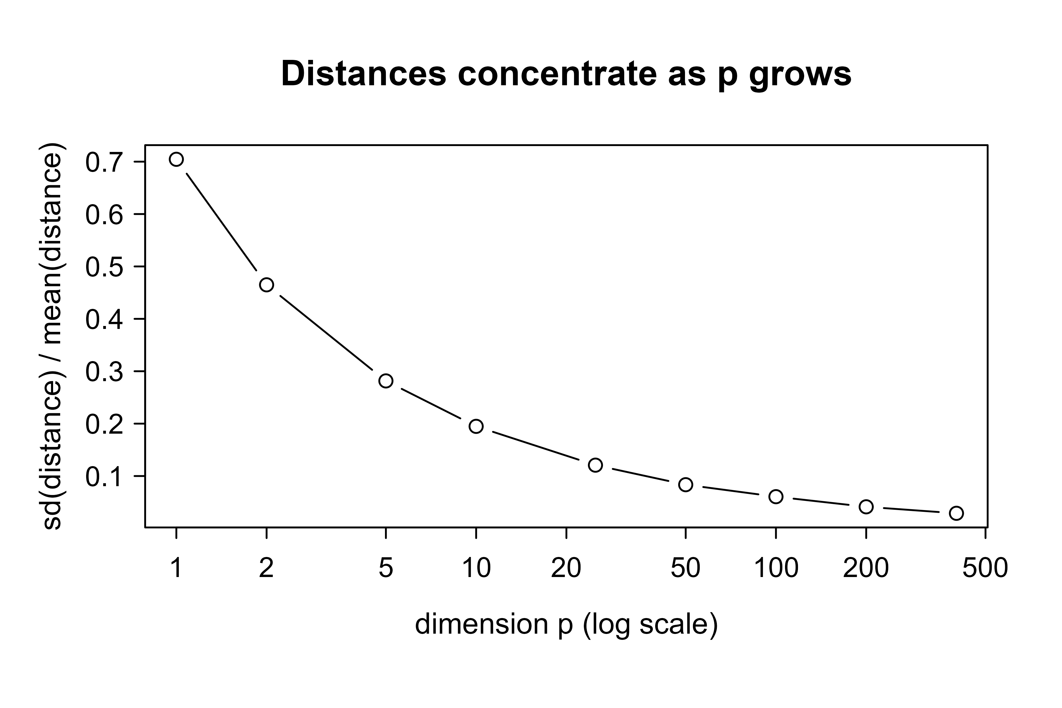
Distances concentrate. A second effect is that pairwise distances become nearly equal as \(p\) grows. Consider points whose coordinates are independent. The squared Euclidean distance between two such points is a sum of \(p\) independent per-coordinate contributions, so by a law-of-large-numbers argument its mean grows like \(p\) while its standard deviation grows only like \(\sqrt{p}\). The ratio of spread to typical distance therefore shrinks like \(1/\sqrt{p}\),
\[
\frac{\text{sd of distance}}{\text{mean of distance}} \to 0 \quad \text{as } p \to \infty.
\]
More precisely, let \(X\) and \(Z\) have independent coordinates with finite variance and let \(D_p^2 = \sum_{j=1}^p (X_j - Z_j)^2\). The summands are independent with common mean \(\mu = \mathbb{E}[(X_j - Z_j)^2]\) and common variance \(\tau^2 = \operatorname{Var}((X_j - Z_j)^2)\), so \(\mathbb{E}[D_p^2] = p\mu\) and \(\operatorname{Var}(D_p^2) = p\tau^2\). The coefficient of variation of the squared distance is then
which is the formal version of the concentration claim and shows the \(1/\sqrt{p}\) rate. A consequence (Beyer et al., 1999) is that the ratio of the farthest to the nearest point distance from a query tends to \(1\) in probability: \(\operatorname{dist}_{\max} / \operatorname{dist}_{\min} \to 1\). When the nearest and farthest neighbors of a query are almost the same distance away, the ranking that kNN depends on carries little information. This is why kNN often performs poorly in high dimensions unless the data lie on a low-dimensional structure or the features are reduced first.
Show code
set.seed(11)cv_distance<-function(p, n=2000){A<-matrix(runif(n*p), ncol =p)B<-matrix(runif(n*p), ncol =p)d<-sqrt(rowSums((A-B)^2))# Euclidean distance per pairsd(d)/mean(d)}ps<-c(1, 2, 5, 10, 25, 50, 100, 200, 400)cv<-sapply(ps, cv_distance)plot(ps, cv, type ="b", log ="x", xlab ="dimension p (log scale)", ylab ="sd(distance) / mean(distance)", main ="Distances concentrate as p grows")
Distance concentration: as the dimension p grows, the coefficient of variation of the pairwise Euclidean distance between independent uniform points shrinks like one over sqrt(p), confirming the concentration result. Nearest and farthest neighbors become indistinguishable.
Key idea
In high dimensions, “near” and “far” stop meaning much. The neighborhood needed to gather enough points spans almost the whole feature range, and all points sit at roughly the same distance. kNN’s core assumption (nearby points are similar) quietly fails, so reduce dimensionality or drop irrelevant features before reaching for kNN.
Having seen how kNN behaves in theory, we turn to the choices that decide whether it works in practice.
17.4 Practical Considerations
17.4.1 Standardization
Because distance mixes all features together, a feature measured on a large numeric scale dominates the distance and crowds out the others. A variable in dollars (range in the thousands) will swamp a variable that is a proportion (range \(0\) to \(1\)). Standardizing each feature to zero mean and unit variance (or scaling to a common range) puts the features on comparable footing before computing distances. This step is essential for kNN, not optional. The Mahalanobis distance addresses the same issue internally by dividing out the covariance.
Warning
Compute the standardization (the means and standard deviations) on the training set only, then apply those same values to the test set. Standardizing the full dataset before splitting leaks information from the test set into training and inflates your performance estimate. The simulation below follows the correct order.
17.4.2 Ties
Two kinds of ties arise. A tie in distance (two training points equally far from the query, with only one slot left in the neighborhood) is usually broken at random or by index order. A tie in the vote (equal class counts) can be broken at random, by choosing the class of the single nearest neighbor, or by using an odd \(k\) in two-class problems to avoid the tie entirely. The class::knn function in R breaks voting ties at random, so results can vary run to run unless a seed is set.
17.4.3 Computational cost
A naive query compares the point to all \(n\) training points in \(O(np)\) time, then selects the \(k\) smallest distances. For \(m\) queries this is \(O(mnp)\), which is acceptable for small data but expensive at scale. Memory is also a concern, since the whole training set must be retained.
17.4.4 kd-trees and ball-trees
Spatial data structures speed up neighbor search by avoiding a full scan. A kd-tree recursively partitions the space with axis-aligned splits; a query descends the tree and uses the partition geometry to prune branches that cannot contain a nearer neighbor. Average query cost can approach \(O(\log n)\) in low dimensions. A ball-tree partitions the data into nested hyperspheres and prunes using the triangle inequality; it tends to hold up better than a kd-tree as \(p\) grows. Both degrade toward the cost of brute force in high dimensions, which is another face of the curse of dimensionality. When exact search is too slow, approximate nearest-neighbor methods trade a small loss in accuracy for large speedups.
17.5 Simulation
The ideas above are easier to trust once you see them. We illustrate the bias-variance tradeoff and the decision boundary on simulated two-class data in two dimensions. The two classes are drawn from Gaussian clusters with overlapping support, so the Bayes error is nonzero and no classifier can drive the test error to zero. Working in two dimensions lets us plot the decision boundary directly and keeps the curse of dimensionality at bay, so the bias-variance story comes through cleanly.
We first generate a training set and a larger test set, then standardize both using statistics computed from the training set alone, as the warning above recommends.
Show code
set.seed(1)# Two classes, each a mixture of Gaussian blobs in 2-D.gen_data<-function(n_per_class){# class 0 centersc0<-rbind(c(-1, -1), c(1.5, -1.5))# class 1 centersc1<-rbind(c(1, 1.2), c(-1.5, 1.5))draw<-function(centers, n, label){idx<-sample(seq_len(nrow(centers)), n, replace =TRUE)pts<-centers[idx, , drop =FALSE]+matrix(rnorm(2*n, sd =0.9), ncol =2)data.frame(x1 =pts[, 1], x2 =pts[, 2], y =factor(label))}rbind(draw(c0, n_per_class, 0),draw(c1, n_per_class, 1))}train<-gen_data(150)test<-gen_data(500)# Standardize features using the training mean and sd.mu<-colMeans(train[, c("x1", "x2")])sdv<-apply(train[, c("x1", "x2")], 2, sd)scale_xy<-function(df){out<-dfout$x1<-(df$x1-mu["x1"])/sdv["x1"]out$x2<-(df$x2-mu["x2"])/sdv["x2"]out}train_s<-scale_xy(train)test_s<-scale_xy(test)
17.5.1 Test error versus k
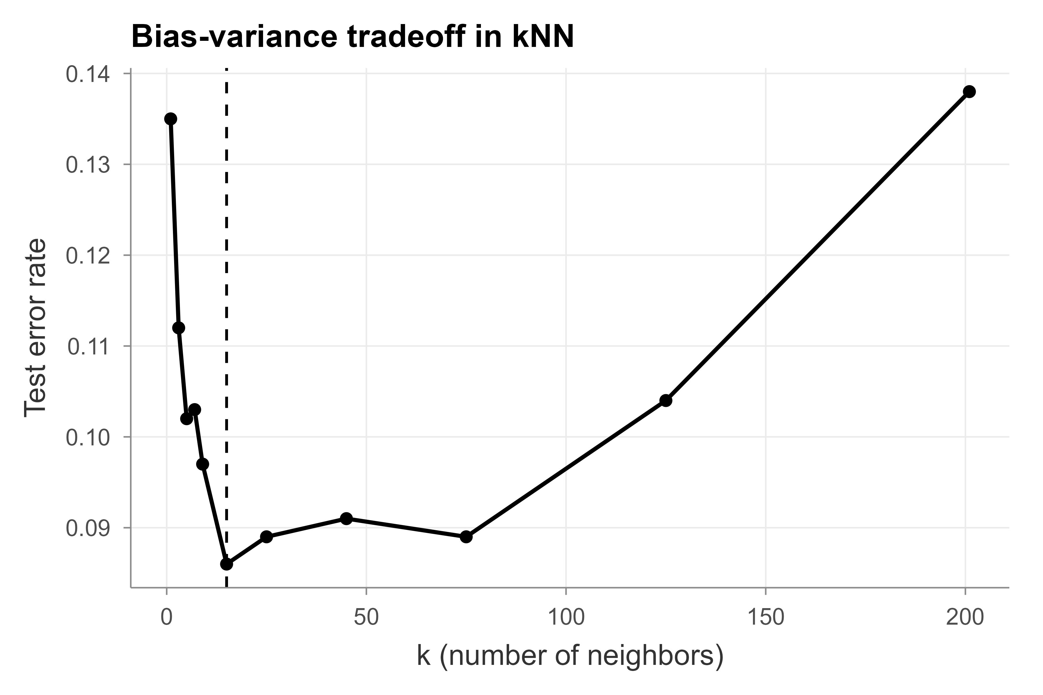
We fit kNN for a grid of \(k\) and record the test error. Table 17.1 lists the test error for each candidate \(k\), and the resulting curve is the U-shape predicted by the bias-variance decomposition: very small \(k\) overfits (high variance), very large \(k\) underfits (high bias).
Show code
library(class)ks<-c(1, 3, 5, 7, 9, 15, 25, 45, 75, 125, 201)train_X<-train_s[, c("x1", "x2")]test_X<-test_s[, c("x1", "x2")]set.seed(2)err<-sapply(ks, function(k){pred<-knn(train =train_X, test =test_X, cl =train_s$y, k =k)mean(pred!=test_s$y)})err_tab<-data.frame(k =ks, test_error =round(err, 4))knitr::kable(err_tab, caption ="kNN test error as a function of k. The error is high for very small k (high variance), reaches a minimum at a moderate k, and rises again for large k (high bias).")
Table 17.1: kNN test error as a function of k. The error is high for very small k (high variance), reaches a minimum at a moderate k, and rises again for large k (high bias).
k
test_error
1
0.135
3
0.112
5
0.102
7
0.103
9
0.097
15
0.086
25
0.089
45
0.091
75
0.089
125
0.104
201
0.138
Figure 17.1 plots the same numbers, making the U-shape and the location of the best \(k\) easy to read off.
Show code
library(ggplot2)best_k<-err_tab$k[which.min(err_tab$test_error)]ggplot(err_tab, aes(x =k, y =test_error))+geom_line()+geom_point()+geom_vline(xintercept =best_k, linetype ="dashed")+labs( x ="k (number of neighbors)", y ="Test error rate", title ="Bias-variance tradeoff in kNN")
Figure 17.1: Test error rate of the kNN classifier as a function of the number of neighbors k. The dashed vertical line marks the k with the lowest test error; the curve is high at small k (high variance) and rises again at large k (high bias).
17.5.2 Decision boundaries
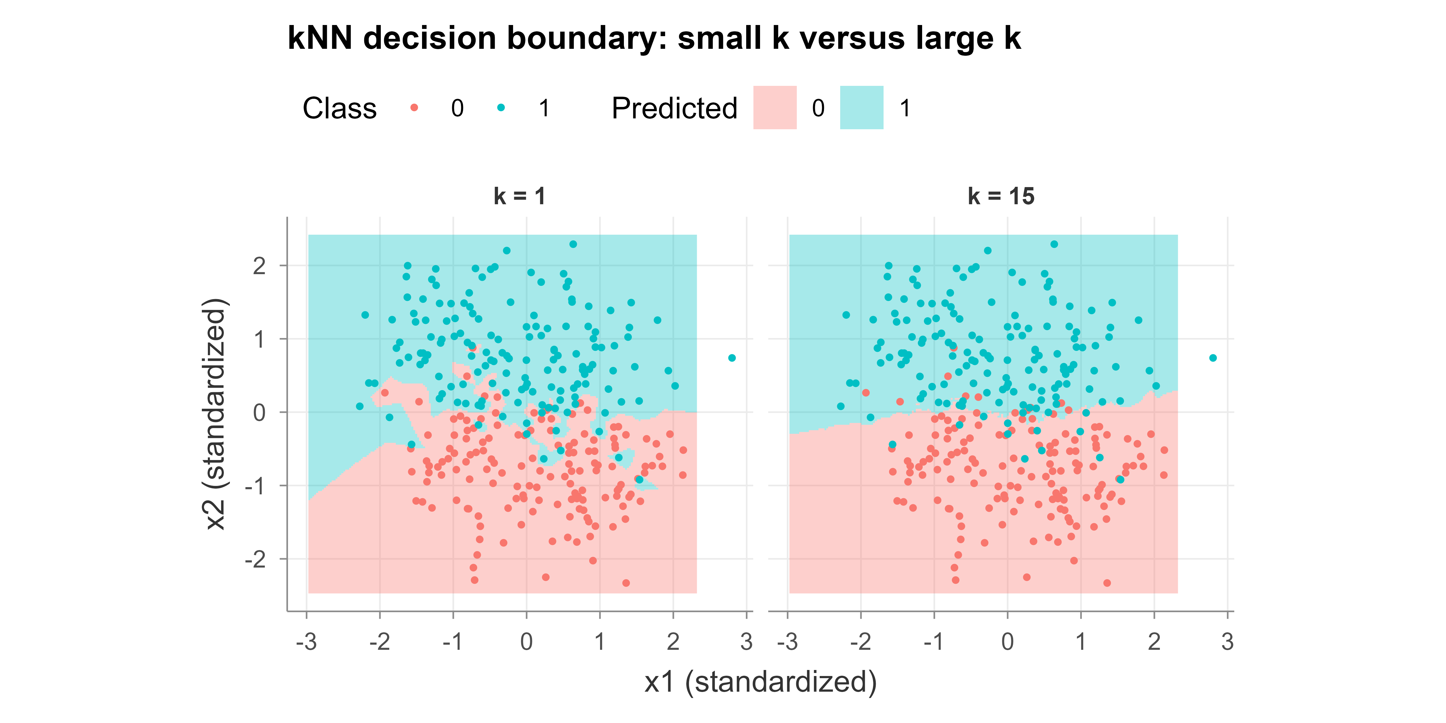
To see the effect of \(k\) directly, we color a fine grid of the feature space by the predicted class for a small \(k\) and a large \(k\). Figure 17.2 shows the two boundaries side by side: the small-\(k\) boundary is jagged and follows individual points, while the large-\(k\) boundary is smooth and stable.
Show code
# Grid over the (standardized) feature space.g1<-seq(min(test_X$x1), max(test_X$x1), length.out =200)g2<-seq(min(test_X$x2), max(test_X$x2), length.out =200)grid<-expand.grid(x1 =g1, x2 =g2)boundary_df<-function(k){set.seed(3)pred<-knn(train =train_X, test =grid, cl =train_s$y, k =k)data.frame(grid, pred =pred, k =paste0("k = ", k))}bd<-rbind(boundary_df(1), boundary_df(best_k))pts<-data.frame( x1 =rep(train_s$x1, 2), x2 =rep(train_s$x2, 2), y =rep(train_s$y, 2), k =rep(c("k = 1", paste0("k = ", best_k)), each =nrow(train_s)))ggplot(bd, aes(x =x1, y =x2))+geom_raster(aes(fill =pred), alpha =0.35)+geom_point(data =pts, aes(color =y), size =0.7)+facet_wrap(~k)+labs( x ="x1 (standardized)", y ="x2 (standardized)", fill ="Predicted", color ="Class", title ="kNN decision boundary: small k versus large k")+coord_equal()
Figure 17.2: kNN decision boundaries for a small k (left) and the cross-validated-best k (right) on the simulated two-class data. Shaded regions show the predicted class over a fine grid; points are the standardized training data. The small-k boundary is jagged (high variance) and the larger-k boundary is smooth (lower variance).
The left panel (\(k = 1\)) carves out small islands around individual training points, a signature of high variance. The right panel (the cross-validated-best \(k\) from the error table) gives a smoother boundary that generalizes better to the test set. Notice that these two pictures are the same phenomenon as the two ends of the U-shaped error curve: the jagged boundary is what overfitting looks like geometrically, and the smooth one is the balance that cross-validation found.
17.6 Practical Notes
The chapter’s advice condenses into a short checklist. Keep these in mind whenever you apply kNN:
Always standardize the features before computing distances, unless you use a scale-invariant metric like Mahalanobis.
Choose \(k\) by cross-validation rather than by a rule of thumb. The optimal \(k\) depends on the noise level and the sample size.
Use an odd \(k\) for two-class problems to reduce voting ties.
Reduce dimensionality when \(p\) is large. Feature selection or a projection (for example PCA, discussed in the dimension reduction chapter, Chapter 27) can restore the locality that kNN needs.
Mind the prediction cost. For large training sets, use a kd-tree or ball-tree (available through the FNN package in R), or an approximate nearest-neighbor library.
kNN handles multiclass naturally through the majority vote, with no change to the algorithm.
Class imbalance distorts the vote: a rare class is easily outvoted. Distance weighting, resampling, or per-class thresholds can help; see the class imbalance chapter (Chapter 80) for a fuller treatment.
17.7 Further Reading
Cover, T. and Hart, P. (1967). Nearest neighbor pattern classification. Foundational analysis of the \(1\)-NN rule and its asymptotic error bound.
Beyer, K., Goldstein, J., Ramakrishnan, R., and Shaft, U. (1999). When is “nearest neighbor” meaningful? Formalizes distance concentration and the collapse of the nearest-to-farthest ratio in high dimensions.
Fix, E. and Hodges, J. L. (1951). Discriminatory analysis, nonparametric discrimination. The original technical report introducing nonparametric nearest-neighbor classification.
Hastie, T., Tibshirani, R., and Friedman, J. (2009). The Elements of Statistical Learning, 2nd edition. See the treatment of kNN, the bias-variance decomposition, and the curse of dimensionality.
James, G., Witten, D., Hastie, T., and Tibshirani, R. (2013). An Introduction to Statistical Learning. Accessible introduction to kNN classification and the choice of \(k\).
Lazy learning is the opposite of eager learning. An eager method (like linear regression) does its hard work up front, distilling the data into coefficients, and then predicts cheaply. A lazy method postpones all the work to query time and keeps the full training set around. Neither is better in general; the right choice depends on whether you predict often or rarely and how much data you can afford to store.↩︎
Here \(n\) is the number of training examples and \(p\) is the number of features, so \(x_i\) is the vector of features for the \(i\)th example and \(y_i\) is its response. We use this notation throughout the book.↩︎
The Bayes classifier is the best any method could do if the true conditional probabilities were known exactly. Its error rate, the Bayes error, is the irreducible floor set by the overlap between classes. kNN tries to estimate those conditional probabilities from local frequencies.↩︎
Cross-validation splits the training data into folds, fits with each candidate \(k\) on all-but-one fold, and measures error on the held-out fold, averaging over folds. The \(k\) with the lowest average held-out error is selected. This estimates generalization error without touching the test set.↩︎
Source Code
# k-Nearest Neighbors {#sec-knn}```{r}#| include: falsesource("_common.R")```Imagine you move to a new town and want to guess whether a house will sell quickly. A reasonable first instinct is to look at the handful of most similar houses nearby (same size, same neighborhood, same age) and see what happened to them. If most of those sold fast, you predict yours will too. That everyday reasoning is exactly the k-Nearest Neighbors algorithm: predict by looking at the closest known examples and copying what they did.This chapter builds that intuition into a precise method. You will learn how kNN turns "look at similar cases" into a formula for both classification and regression, why the single tuning parameter $k$ controls the tradeoff between fitting noise and oversmoothing, why the method breaks down when the number of features is large (the curse of dimensionality), and the practical steps (standardizing features, choosing $k$ by cross-validation, speeding up search) that make it work in practice. We close with a simulation that shows the bias-variance tradeoff and the decision boundary directly.kNN is one of the most fundamental predictive methods. It is the most direct embodiment of the principle that nearby points should have similar responses, and the same principle reappears, in more refined form, in the kernel smoothing (@sec-kernel) and local regression (@sec-local) methods covered earlier. Because it is so transparent, kNN is a useful baseline: if an elaborate model cannot beat nearest neighbors on your problem, that is worth knowing.## Intuitionk-Nearest Neighbors (kNN) is one of the simplest predictive methods, and it is a useful reference point for understanding more elaborate models. The idea is direct: to predict the response at a query point $x$, look at the $k$ training points closest to $x$ and let them vote (for classification) or average their responses (for regression).::: {.callout-tip title="Intuition"}A prediction is just a poll of the neighbors. For classification the neighbors vote on a class; for regression they report a number and you take the average. Everything else in this chapter is about who counts as a neighbor and how many to ask.:::kNN sits in a particular corner of the prediction landscape:- It is nonparametric. The method does not assume a fixed functional form (no linear predictor, no fixed number of coefficients). The complexity of the fitted function grows with the data.- It is instance-based (also called memory-based). Rather than summarizing the data into a small set of parameters, kNN keeps the training set and consults it at prediction time.- It does no training in the usual sense. There is no optimization step that fits parameters. All of the work happens when a prediction is requested, so the cost shifts from fit time to query time. This is sometimes called lazy learning.^[Lazy learning is the opposite of eager learning. An eager method (like linear regression) does its hard work up front, distilling the data into coefficients, and then predicts cheaply. A lazy method postpones all the work to query time and keeps the full training set around. Neither is better in general; the right choice depends on whether you predict often or rarely and how much data you can afford to store.]Because it makes few assumptions, kNN can approximate very irregular decision boundaries. The price is that it needs enough data to populate the neighborhood of every query point, and it is sensitive to the scale of the features and to the number of features. Those tradeoffs are the subject of the rest of this chapter.::: {.callout-tip title="When to use this"}kNN is a strong choice when you have a moderate number of features, plenty of training examples relative to the number of features, and a decision boundary that may be irregular. It is a poor choice when features are high-dimensional, when predictions must be very fast on a large training set, or when many features are irrelevant (they add noise to the distance).:::## The kNN Estimator### SetupWe have training data $(x_1, y_1), \dots, (x_n, y_n)$ with $x_i \in \mathbb{R}^p$, meaning each example has $p$ features and a known response.^[Here $n$ is the number of training examples and $p$ is the number of features, so $x_i$ is the vector of features for the $i$th example and $y_i$ is its response. We use this notation throughout the book.] For a query point $x$, let $N_k(x)$ denote the index set of the $k$ training points nearest to $x$ under a chosen distance $d(\cdot, \cdot)$. Formally, $N_k(x)$ contains the indices of the $k$ smallest values among $d(x, x_1), \dots, d(x, x_n)$.With the neighborhood $N_k(x)$ defined, the prediction rule depends only on what we do with the responses inside it. Classification and regression differ just in that final step.### ClassificationFor a classification problem with classes $c \in \{1, \dots, C\}$, kNN estimates the class posterior probability by the fraction of neighbors in each class:$$\hat p(y = c \mid x) = \frac{1}{k} \sum_{i \in N_k(x)} \mathbb{1}(y_i = c).$$The predicted class is the majority vote among the neighbors,$$\hat y(x) = \arg\max_{c} \ \hat p(y = c \mid x) = \arg\max_{c} \ \sum_{i \in N_k(x)} \mathbb{1}(y_i = c).$$In words, the estimated probability that $x$ belongs to class $c$ is simply the share of its $k$ neighbors that carry label $c$, and the prediction is whichever class wins that local poll.This is a plug-in approximation to the Bayes classifier, which assigns $x$ to $\arg\max_c p(y = c \mid x)$.^[The Bayes classifier is the best any method could do if the true conditional probabilities were known exactly. Its error rate, the Bayes error, is the irreducible floor set by the overlap between classes. kNN tries to estimate those conditional probabilities from local frequencies.] As $n \to \infty$ and $k \to \infty$ with $k/n \to 0$, the kNN classifier is consistent, and its error rate converges to the Bayes rate under mild conditions. The classic finite-$k$ result of Cover and Hart (1967) shows that the asymptotic error of the $1$-NN rule is at most twice the Bayes error.### The Cover-Hart bound, derivedThe two-times-Bayes guarantee is worth deriving, because the argument is short and shows exactly where the factor of two comes from. Restrict to two classes, $c \in \{1, 2\}$, and write the conditional probability of class $1$ at a point $x$ as $\eta(x) = p(y = 1 \mid x)$. The Bayes classifier predicts the more probable class, so its conditional error at $x$ is$$r^*(x) = \min\{\eta(x),\, 1 - \eta(x)\},$$and the Bayes risk is $R^* = \mathbb{E}_x[r^*(x)]$.Consider the $1$-NN rule and a fixed query $x$ with nearest neighbor $x_{(1)}$ carrying label $y_{(1)}$. As $n \to \infty$, the nearest neighbor converges to the query, $x_{(1)} \to x$ almost surely, provided $x$ is in the support of the feature distribution (this is the key regularity condition: a nearest neighbor really does get arbitrarily close once data are dense). Assuming $\eta$ is continuous, $\eta(x_{(1)}) \to \eta(x)$. The $1$-NN rule errs at $x$ when the test label and the neighbor label disagree. Conditional on $x$ and $x_{(1)}$, the test label is class $1$ with probability $\eta(x)$ and the neighbor label is class $1$ with probability $\eta(x_{(1)})$, drawn independently. The conditional error probability is therefore$$r_{\text{1NN}}(x) = \eta(x)\,(1 - \eta(x_{(1)})) + (1 - \eta(x))\,\eta(x_{(1)}).$$Taking the limit $\eta(x_{(1)}) \to \eta(x)$,$$r_{\text{1NN}}(x) \to 2\,\eta(x)\,(1 - \eta(x)).$$ {#eq-knn-1nn-asymptotic}Now bound the right side in terms of the Bayes error $r^*(x) = \min\{\eta, 1-\eta\}$. Writing $\eta = \eta(x)$,$$2\,\eta(1 - \eta) = 2\, r^*(x)\,(1 - r^*(x)) \le 2\, r^*(x),$$since $r^*(x) = \min\{\eta, 1-\eta\}$ gives $\eta(1-\eta) = r^*(x)(1 - r^*(x))$ and $(1 - r^*(x)) \le 1$. Taking expectations over $x$ yields the Cover-Hart bound for the asymptotic $1$-NN risk $R_{\text{1NN}}$,$$R^* \;\le\; R_{\text{1NN}} \;\le\; 2\,R^* (1 - R^*) \;\le\; 2\,R^*.$$ {#eq-knn-cover-hart}The lower bound $R^* \le R_{\text{1NN}}$ is immediate (no rule beats Bayes). The middle expression uses Jensen's inequality: $\mathbb{E}[r^*(1 - r^*)] \le \mathbb{E}[r^*]\,(1 - \mathbb{E}[r^*])$ because $t \mapsto t(1-t)$ is concave. The factor of two in @eq-knn-1nn-asymptotic comes from a single independent draw being used as the prediction: the predictor and the truth each carry the local class noise, and the two noise sources combine. Averaging over $k > 1$ neighbors damps that second noise source, which is why $k$-NN with $k \to \infty$ closes the gap and attains $R^*$ exactly.::: {.callout-important title="Key idea"}Even the crudest version of kNN (a single nearest neighbor) is never more than twice as bad as the theoretical optimum in the large-sample limit. That is a remarkable guarantee for such a simple rule, and it explains why kNN remains a respected baseline.:::### RegressionFor regression, kNN predicts the average response over the neighborhood:$$\hat f(x) = \frac{1}{k} \sum_{i \in N_k(x)} y_i.$$This is a locally constant estimate: within any neighborhood, the fit is a flat line at the local average. It can be viewed as a kernel-weighted average with a uniform weight over the $k$ nearest points and zero weight elsewhere, which connects kNN to the kernel smoothing methods covered earlier in the book (@sec-kernel). The neighborhood is defined by a fixed count $k$ rather than a fixed bandwidth in distance, so the effective window adapts to local data density: it shrinks where data are dense and widens where data are sparse.::: {.callout-note}Kernel smoothing fixes a window width (a bandwidth $h$) and averages whatever falls inside. kNN fixes a count $k$ and lets the window width float. The two are mirror images of the same locally-weighted-averaging idea, and which one behaves better depends on how evenly your data are spread.:::### Distance metricsSo far "nearest" has been left undefined. We now make it precise, because the choice of distance is what determines who the neighbors are. For $x, z \in \mathbb{R}^p$, common choices are:- Euclidean ($L_2$): $d(x, z) = \left( \sum_{j=1}^p (x_j - z_j)^2 \right)^{1/2}$.- Manhattan ($L_1$): $d(x, z) = \sum_{j=1}^p |x_j - z_j|$.- Minkowski ($L_q$): $d(x, z) = \left( \sum_{j=1}^p |x_j - z_j|^q \right)^{1/q}$, which gives Manhattan for $q = 1$ and Euclidean for $q = 2$.- Mahalanobis: $d(x, z) = \left( (x - z)^\top \Sigma^{-1} (x - z) \right)^{1/2}$, where $\Sigma$ is a covariance matrix (often estimated from the data). This metric accounts for correlation among features and for differences in their spread, so it is scale-invariant in a way the others are not.Euclidean distance is the default and works well once features are on comparable scales. Manhattan distance can be more robust when features are noisy or when large coordinate differences should not be squared. Mahalanobis distance is the right tool when features are correlated or measured in very different units, since it folds standardization and decorrelation into the metric itself.### Distance weightingPlain kNN gives every neighbor an equal vote. A refinement weights neighbors by closeness, so that a point right next to $x$ counts more than one at the edge of the neighborhood. With weights $w_i \ge 0$, the weighted estimates are$$\hat p(y = c \mid x) = \frac{\sum_{i \in N_k(x)} w_i \, \mathbb{1}(y_i = c)}{\sum_{i \in N_k(x)} w_i},\qquad\hat f(x) = \frac{\sum_{i \in N_k(x)} w_i \, y_i}{\sum_{i \in N_k(x)} w_i}.$$A common weight is the inverse distance $w_i = 1 / d(x, x_i)$ (with a small offset to avoid division by zero), or a kernel of the distance such as $w_i = K\!\left( d(x, x_i) / h \right)$. Distance weighting reduces the sensitivity to the exact value of $k$, because far-off neighbors contribute little.### kNN as a kernel estimator with an adaptive bandwidthWeighted kNN is exactly the Nadaraya-Watson kernel regression estimator (see @sec-kernel) with a data-adaptive bandwidth. Recall the Nadaraya-Watson estimate $\hat f(x) = \sum_i K_h(x, x_i)\, y_i / \sum_i K_h(x, x_i)$. Set the bandwidth equal to the distance to the $k$th nearest neighbor, $h_k(x) = d(x, x_{(k)})$, and use a kernel supported on the unit ball. Then $K_{h_k(x)}(x, x_i)$ is nonzero only for the $k$ nearest points, and the kernel estimate becomes the weighted kNN formula above. Choosing the box kernel $K(u) = \mathbb{1}(\|u\| \le 1)$ recovers plain (unweighted) kNN, while a smooth kernel such as the tri-cube or Epanechnikov recovers distance-weighted kNN. The defining feature of kNN within this family is that the bandwidth $h_k(x)$ varies with location: it is small where data are dense and large where data are sparse. Fixed-bandwidth kernel smoothing makes the opposite choice. This is why kNN keeps a roughly constant variance across the domain (always $k$ effective points) at the cost of a location-dependent bias, whereas a fixed bandwidth keeps a roughly constant bias at the cost of a location-dependent variance.### Fixed-radius neighbors and other variantsA close relative replaces the count $k$ with a radius $\rho$: predict from all training points within distance $\rho$ of the query (fixed-radius near neighbors). This swaps the adaptive-bandwidth behavior back for a fixed bandwidth and can return an empty neighborhood in sparse regions, which must be handled (for example by falling back to the single nearest point). Other practical variants include condensed and edited nearest neighbors, which prune the training set to a smaller representative subset to cut query cost and remove mislabeled points, and prototype methods (such as learning vector quantization) that replace the raw training set with a small set of learned centers.### Failure modeskNN breaks in a few characteristic ways, each traceable to the assumptions above. Irrelevant features inflate the distance with noise and destroy locality; because every feature contributes to $d$, a handful of useless coordinates can dominate the metric (this is distinct from, but compounded by, the curse of dimensionality). Unscaled features let the largest-range variable dictate the neighborhood, as discussed under standardization. Class imbalance lets a common class win the vote even far from its true region. Heavy local label noise propagates directly into predictions at small $k$, since there is no averaging to suppress it. And on the boundary of the data support the neighborhood becomes one-sided, so the linear term in the Taylor expansion no longer cancels and the bias picks up a first-order (rather than second-order) contribution, the same boundary bias that motivates local-linear regression over local-constant fits in @sec-local.## Bias, Variance, and the Choice of kThe parameter $k$ controls the smoothness of the fit and is the main knob in kNN. Understanding how it works is the heart of using the method well, so we take it slowly: first the intuition for small and large $k$, then an exact derivation for regression, and then the special difficulty that high dimensions create.### Small versus large kWith $k = 1$, the prediction at any training point is that point's own label, so the training error is zero, and the decision boundary is highly irregular, tracking individual points. This is low bias and high variance: the fit closely follows the data, but a small change in the training set can change the prediction substantially.With large $k$, the prediction averages over a wide region. The boundary smooths out and becomes more stable across training sets, but it can miss real local structure. This is high bias and low variance. In the limit $k = n$, every query receives the same prediction (the overall majority class or the global mean), which is the most biased and least variable estimate possible.::: {.callout-warning}A training error of zero (which $k = 1$ always achieves) is not a sign of a good model. It means the model has memorized the training set, including its noise. The quantity to watch is error on held-out data, not training error.:::### A regression derivationThe bias-variance behavior can be made precise for regression. Assume $y_i = f(x_i) + \varepsilon_i$ with $\mathbb{E}[\varepsilon_i] = 0$ and $\operatorname{Var}(\varepsilon_i) = \sigma^2$, errors independent. Treat the neighborhood points as fixed and let $\hat f(x) = \frac{1}{k} \sum_{i \in N_k(x)} y_i$. Then$$\mathbb{E}[\hat f(x)] = \frac{1}{k} \sum_{i \in N_k(x)} f(x_i),\qquad\operatorname{Var}(\hat f(x)) = \frac{\sigma^2}{k}.$$The expected squared error at $x$ decomposes as$$\mathbb{E}\left[ (y - \hat f(x))^2 \right]= \sigma^2+ \underbrace{\left( f(x) - \frac{1}{k} \sum_{i \in N_k(x)} f(x_i) \right)^2}_{\text{bias}^2}+ \underbrace{\frac{\sigma^2}{k}}_{\text{variance}}.$$To see where these two expressions come from, write $\hat f(x) = \frac{1}{k}\sum_{i \in N_k(x)} y_i = \frac{1}{k}\sum_{i \in N_k(x)} \bigl(f(x_i) + \varepsilon_i\bigr)$ with the neighbor indices held fixed. Linearity of expectation and $\mathbb{E}[\varepsilon_i] = 0$ give the mean directly. For the variance, the $f(x_i)$ are constants, so only the noise contributes, and independence of the $\varepsilon_i$ turns the variance of the sum into the sum of variances,$$\operatorname{Var}\!\bigl(\hat f(x)\bigr)= \frac{1}{k^2} \sum_{i \in N_k(x)} \operatorname{Var}(\varepsilon_i)= \frac{1}{k^2}\, k\, \sigma^2= \frac{\sigma^2}{k}.$$The variance term $\sigma^2 / k$ falls as $k$ grows: averaging more points reduces the noise. The squared bias term tends to grow with $k$, because larger neighborhoods reach farther from $x$, where $f(x_i)$ can differ from $f(x)$. The sum of these two terms is the familiar U-shaped curve in $k$, and the best $k$ balances them. In practice $k$ is chosen by cross-validation.^[Cross-validation splits the training data into folds, fits with each candidate $k$ on all-but-one fold, and measures error on the held-out fold, averaging over folds. The $k$ with the lowest average held-out error is selected. This estimates generalization error without touching the test set.] The effective number of parameters of a kNN fit is often described as roughly $n / k$, which makes the role of $k$ as a complexity control explicit.::: {.callout-note title="Effective degrees of freedom, made precise"}The estimate at the training points is linear in the responses, $\hat{\mathbf{f}} = \mathbf{S}\mathbf{y}$, where the smoother matrix $\mathbf{S}$ has entry $S_{ij} = 1/k$ if $j \in N_k(x_i)$ and $0$ otherwise. The standard definition of effective degrees of freedom for a linear smoother is $\operatorname{df} = \operatorname{tr}(\mathbf{S})$. Each diagonal entry $S_{ii}$ equals $1/k$ because a point is always its own nearest neighbor, so$$\operatorname{df} = \operatorname{tr}(\mathbf{S}) = \sum_{i=1}^n \frac{1}{k} = \frac{n}{k}.$$This makes the "$n/k$ effective parameters" statement exact under the usual smoother-trace definition, and it is the same notion of degrees of freedom used for splines and other linear smoothers elsewhere in the book.:::### How fast does the bias grow, and the optimal $k$The bias depends on how far the neighbors reach and how curved $f$ is. We can make the rate explicit. Suppose the $n$ training inputs are spread with roughly uniform density in $\mathbb{R}^p$, and $f$ is smooth with bounded second derivatives near $x$. The $k$ nearest neighbors fill a ball whose radius $r_k$ must enclose a fraction $k/n$ of the data, so its volume scales like $k/n$ and, since volume in $p$ dimensions grows like $r^p$,$$r_k \asymp \left( \frac{k}{n} \right)^{1/p}.$$A second-order Taylor expansion of $f$ around $x$ gives $f(x_i) - f(x) \approx \nabla f(x)^\top (x_i - x) + \tfrac{1}{2}(x_i - x)^\top H (x_i - x)$. Averaged over a roughly symmetric neighborhood the linear term largely cancels, leaving a bias of order $r_k^2$. Therefore$$\operatorname{bias}^2 \asymp r_k^4 \asymp \left( \frac{k}{n} \right)^{4/p},\qquad\operatorname{Var} = \frac{\sigma^2}{k}.$$The mean squared error is the sum, $\text{MSE}(k) \asymp (k/n)^{4/p} + \sigma^2/k$. Minimizing over $k$ by differentiating and setting the derivative to zero,$$\frac{4}{p}\,\frac{k^{4/p - 1}}{n^{4/p}} - \frac{\sigma^2}{k^2} = 0\quad\Longrightarrow\quadk^{\,4/p + 1} \asymp n^{4/p},$$so the optimal neighborhood size and the resulting error rate are$$k^* \asymp n^{\frac{4}{p+4}},\qquad\text{MSE}(k^*) \asymp n^{-\frac{4}{p+4}}.$$ {#eq-knn-optimal-k}Two lessons follow from @eq-knn-optimal-k. First, the optimal $k$ grows with $n$ (slowly), so cross-validation should be allowed to pick larger $k$ as the sample grows. Second, the convergence rate $n^{-4/(p+4)}$ is the nonparametric rate for twice-differentiable functions, and it slows dramatically as $p$ increases: this is the curse of dimensionality stated as a rate, and it is the same rate achieved by kernel and local-linear smoothers, confirming that kNN is a member of that family rather than something faster.::: {.callout-tip}Read $n/k$ as the model's complexity. Small $k$ means many effective parameters (a flexible, wiggly fit); large $k$ means few (a rigid, smooth fit). This is the same dial as the degrees of freedom in a spline or the depth of a tree, just expressed through the neighborhood size.:::### The curse of dimensionalitykNN relies on neighbors being genuinely close to the query point. In high dimensions this becomes hard to satisfy, for two related reasons.Neighborhoods are not local. Suppose the $n$ training points are spread uniformly in the unit cube $[0,1]^p$. To capture a fraction $r$ of the data in a cubical neighborhood, the side length of that cube must be about$$e_p(r) = r^{1/p}.$$For example, to capture $r = 1\%$ of the data: in $p = 1$ dimension the neighborhood spans $0.01$ of each axis, but in $p = 10$ dimensions it spans $0.01^{1/10} \approx 0.63$ of each axis, and in $p = 100$ it spans $0.01^{1/100} \approx 0.95$. The "local" neighborhood is no longer local at all; it reaches across most of the range of every feature, so the estimate is no longer based on nearby points.Distances concentrate. A second effect is that pairwise distances become nearly equal as $p$ grows. Consider points whose coordinates are independent. The squared Euclidean distance between two such points is a sum of $p$ independent per-coordinate contributions, so by a law-of-large-numbers argument its mean grows like $p$ while its standard deviation grows only like $\sqrt{p}$. The ratio of spread to typical distance therefore shrinks like $1/\sqrt{p}$,$$\frac{\text{sd of distance}}{\text{mean of distance}} \to 0 \quad \text{as } p \to \infty.$$More precisely, let $X$ and $Z$ have independent coordinates with finite variance and let $D_p^2 = \sum_{j=1}^p (X_j - Z_j)^2$. The summands are independent with common mean $\mu = \mathbb{E}[(X_j - Z_j)^2]$ and common variance $\tau^2 = \operatorname{Var}((X_j - Z_j)^2)$, so $\mathbb{E}[D_p^2] = p\mu$ and $\operatorname{Var}(D_p^2) = p\tau^2$. The coefficient of variation of the squared distance is then$$\frac{\operatorname{sd}(D_p^2)}{\mathbb{E}[D_p^2]} = \frac{\sqrt{p}\,\tau}{p\,\mu} = \frac{\tau}{\mu}\,\frac{1}{\sqrt{p}} \;\to\; 0,$$ {#eq-knn-concentration}which is the formal version of the concentration claim and shows the $1/\sqrt{p}$ rate. A consequence (Beyer et al., 1999) is that the ratio of the farthest to the nearest point distance from a query tends to $1$ in probability: $\operatorname{dist}_{\max} / \operatorname{dist}_{\min} \to 1$. When the nearest and farthest neighbors of a query are almost the same distance away, the ranking that kNN depends on carries little information. This is why kNN often performs poorly in high dimensions unless the data lie on a low-dimensional structure or the features are reduced first.```{r knn-concentration, fig.width=6, fig.height=4, fig.cap="Distance concentration: as the dimension p grows, the coefficient of variation of the pairwise Euclidean distance between independent uniform points shrinks like one over sqrt(p), confirming the concentration result. Nearest and farthest neighbors become indistinguishable."}set.seed(11)cv_distance <-function(p, n =2000) { A <-matrix(runif(n * p), ncol = p) B <-matrix(runif(n * p), ncol = p) d <-sqrt(rowSums((A - B)^2)) # Euclidean distance per pairsd(d) /mean(d)}ps <-c(1, 2, 5, 10, 25, 50, 100, 200, 400)cv <-sapply(ps, cv_distance)plot(ps, cv, type ="b", log ="x",xlab ="dimension p (log scale)",ylab ="sd(distance) / mean(distance)",main ="Distances concentrate as p grows")```::: {.callout-important title="Key idea"}In high dimensions, "near" and "far" stop meaning much. The neighborhood needed to gather enough points spans almost the whole feature range, and all points sit at roughly the same distance. kNN's core assumption (nearby points are similar) quietly fails, so reduce dimensionality or drop irrelevant features before reaching for kNN.:::Having seen how kNN behaves in theory, we turn to the choices that decide whether it works in practice.## Practical Considerations### StandardizationBecause distance mixes all features together, a feature measured on a large numeric scale dominates the distance and crowds out the others. A variable in dollars (range in the thousands) will swamp a variable that is a proportion (range $0$ to $1$). Standardizing each feature to zero mean and unit variance (or scaling to a common range) puts the features on comparable footing before computing distances. This step is essential for kNN, not optional. The Mahalanobis distance addresses the same issue internally by dividing out the covariance.::: {.callout-warning}Compute the standardization (the means and standard deviations) on the training set only, then apply those same values to the test set. Standardizing the full dataset before splitting leaks information from the test set into training and inflates your performance estimate. The simulation below follows the correct order.:::### TiesTwo kinds of ties arise. A tie in distance (two training points equally far from the query, with only one slot left in the neighborhood) is usually broken at random or by index order. A tie in the vote (equal class counts) can be broken at random, by choosing the class of the single nearest neighbor, or by using an odd $k$ in two-class problems to avoid the tie entirely. The `class::knn` function in R breaks voting ties at random, so results can vary run to run unless a seed is set.### Computational costA naive query compares the point to all $n$ training points in $O(np)$ time, then selects the $k$ smallest distances. For $m$ queries this is $O(mnp)$, which is acceptable for small data but expensive at scale. Memory is also a concern, since the whole training set must be retained.### kd-trees and ball-treesSpatial data structures speed up neighbor search by avoiding a full scan. A kd-tree recursively partitions the space with axis-aligned splits; a query descends the tree and uses the partition geometry to prune branches that cannot contain a nearer neighbor. Average query cost can approach $O(\log n)$ in low dimensions. A ball-tree partitions the data into nested hyperspheres and prunes using the triangle inequality; it tends to hold up better than a kd-tree as $p$ grows. Both degrade toward the cost of brute force in high dimensions, which is another face of the curse of dimensionality. When exact search is too slow, approximate nearest-neighbor methods trade a small loss in accuracy for large speedups.## SimulationThe ideas above are easier to trust once you see them. We illustrate the bias-variance tradeoff and the decision boundary on simulated two-class data in two dimensions. The two classes are drawn from Gaussian clusters with overlapping support, so the Bayes error is nonzero and no classifier can drive the test error to zero. Working in two dimensions lets us plot the decision boundary directly and keeps the curse of dimensionality at bay, so the bias-variance story comes through cleanly.We first generate a training set and a larger test set, then standardize both using statistics computed from the training set alone, as the warning above recommends.```{r knn-data}set.seed(1)# Two classes, each a mixture of Gaussian blobs in 2-D.gen_data <-function(n_per_class) {# class 0 centers c0 <-rbind(c(-1, -1), c(1.5, -1.5))# class 1 centers c1 <-rbind(c(1, 1.2), c(-1.5, 1.5)) draw <-function(centers, n, label) { idx <-sample(seq_len(nrow(centers)), n, replace =TRUE) pts <- centers[idx, , drop =FALSE] +matrix(rnorm(2* n, sd =0.9), ncol =2)data.frame(x1 = pts[, 1], x2 = pts[, 2], y =factor(label)) }rbind(draw(c0, n_per_class, 0),draw(c1, n_per_class, 1) )}train <-gen_data(150)test <-gen_data(500)# Standardize features using the training mean and sd.mu <-colMeans(train[, c("x1", "x2")])sdv <-apply(train[, c("x1", "x2")], 2, sd)scale_xy <-function(df) { out <- df out$x1 <- (df$x1 - mu["x1"]) / sdv["x1"] out$x2 <- (df$x2 - mu["x2"]) / sdv["x2"] out}train_s <-scale_xy(train)test_s <-scale_xy(test)```### Test error versus kWe fit kNN for a grid of $k$ and record the test error. @tbl-knn-error-table lists the test error for each candidate $k$, and the resulting curve is the U-shape predicted by the bias-variance decomposition: very small $k$ overfits (high variance), very large $k$ underfits (high bias).```{r tbl-knn-error-table}library(class)ks <-c(1, 3, 5, 7, 9, 15, 25, 45, 75, 125, 201)train_X <- train_s[, c("x1", "x2")]test_X <- test_s[, c("x1", "x2")]set.seed(2)err <-sapply(ks, function(k) { pred <-knn(train = train_X, test = test_X, cl = train_s$y, k = k)mean(pred != test_s$y)})err_tab <-data.frame(k = ks, test_error =round(err, 4))knitr::kable( err_tab,caption ="kNN test error as a function of k. The error is high for very small k (high variance), reaches a minimum at a moderate k, and rises again for large k (high bias).")```@fig-knn-error-plot plots the same numbers, making the U-shape and the location of the best $k$ easy to read off.```{r fig-knn-error-plot, fig.width=6, fig.height=4, fig.cap="Test error rate of the kNN classifier as a function of the number of neighbors k. The dashed vertical line marks the k with the lowest test error; the curve is high at small k (high variance) and rises again at large k (high bias)."}library(ggplot2)best_k <- err_tab$k[which.min(err_tab$test_error)]ggplot(err_tab, aes(x = k, y = test_error)) +geom_line() +geom_point() +geom_vline(xintercept = best_k, linetype ="dashed") +labs(x ="k (number of neighbors)",y ="Test error rate",title ="Bias-variance tradeoff in kNN" )```### Decision boundariesTo see the effect of $k$ directly, we color a fine grid of the feature space by the predicted class for a small $k$ and a large $k$. @fig-knn-boundary shows the two boundaries side by side: the small-$k$ boundary is jagged and follows individual points, while the large-$k$ boundary is smooth and stable.```{r fig-knn-boundary, fig.width=8, fig.height=4, fig.cap="kNN decision boundaries for a small k (left) and the cross-validated-best k (right) on the simulated two-class data. Shaded regions show the predicted class over a fine grid; points are the standardized training data. The small-k boundary is jagged (high variance) and the larger-k boundary is smooth (lower variance)."}# Grid over the (standardized) feature space.g1 <-seq(min(test_X$x1), max(test_X$x1), length.out =200)g2 <-seq(min(test_X$x2), max(test_X$x2), length.out =200)grid <-expand.grid(x1 = g1, x2 = g2)boundary_df <-function(k) {set.seed(3) pred <-knn(train = train_X, test = grid, cl = train_s$y, k = k)data.frame(grid, pred = pred, k =paste0("k = ", k))}bd <-rbind(boundary_df(1), boundary_df(best_k))pts <-data.frame(x1 =rep(train_s$x1, 2),x2 =rep(train_s$x2, 2),y =rep(train_s$y, 2),k =rep(c("k = 1", paste0("k = ", best_k)), each =nrow(train_s)))ggplot(bd, aes(x = x1, y = x2)) +geom_raster(aes(fill = pred), alpha =0.35) +geom_point(data = pts, aes(color = y), size =0.7) +facet_wrap(~ k) +labs(x ="x1 (standardized)",y ="x2 (standardized)",fill ="Predicted",color ="Class",title ="kNN decision boundary: small k versus large k" ) +coord_equal()```The left panel ($k = 1$) carves out small islands around individual training points, a signature of high variance. The right panel (the cross-validated-best $k$ from the error table) gives a smoother boundary that generalizes better to the test set. Notice that these two pictures are the same phenomenon as the two ends of the U-shaped error curve: the jagged boundary is what overfitting looks like geometrically, and the smooth one is the balance that cross-validation found.## Practical NotesThe chapter's advice condenses into a short checklist. Keep these in mind whenever you apply kNN:- Always standardize the features before computing distances, unless you use a scale-invariant metric like Mahalanobis.- Choose $k$ by cross-validation rather than by a rule of thumb. The optimal $k$ depends on the noise level and the sample size.- Use an odd $k$ for two-class problems to reduce voting ties.- Reduce dimensionality when $p$ is large. Feature selection or a projection (for example PCA, discussed in the dimension reduction chapter, @sec-dimension-reduction) can restore the locality that kNN needs.- Mind the prediction cost. For large training sets, use a kd-tree or ball-tree (available through the `FNN` package in R), or an approximate nearest-neighbor library.- kNN handles multiclass naturally through the majority vote, with no change to the algorithm.- Class imbalance distorts the vote: a rare class is easily outvoted. Distance weighting, resampling, or per-class thresholds can help; see the class imbalance chapter (@sec-class-imbalance) for a fuller treatment.## Further Reading- Cover, T. and Hart, P. (1967). Nearest neighbor pattern classification. Foundational analysis of the $1$-NN rule and its asymptotic error bound.- Beyer, K., Goldstein, J., Ramakrishnan, R., and Shaft, U. (1999). When is "nearest neighbor" meaningful? Formalizes distance concentration and the collapse of the nearest-to-farthest ratio in high dimensions.- Fix, E. and Hodges, J. L. (1951). Discriminatory analysis, nonparametric discrimination. The original technical report introducing nonparametric nearest-neighbor classification.- Hastie, T., Tibshirani, R., and Friedman, J. (2009). The Elements of Statistical Learning, 2nd edition. See the treatment of kNN, the bias-variance decomposition, and the curse of dimensionality.- James, G., Witten, D., Hastie, T., and Tibshirani, R. (2013). An Introduction to Statistical Learning. Accessible introduction to kNN classification and the choice of $k$.