| Family | What it does | Stores raw data? | Extra cost grows with |
|---|---|---|---|
| Regularization (e.g. EWC, SI) | Penalize moving parameters important to old tasks | No | Parameters (one importance weight each) |
| Rehearsal / replay | Keep a small buffer of old examples and mix them in | Yes (small buffer) | Buffer size |
| Parameter isolation | Dedicate separate parameters (or masks) per task | No | Number of tasks (capacity) |
58 Continual and Lifelong Learning
Most models in this book are trained once. You assemble a dataset, fit, evaluate, and deploy. Continual learning (also called lifelong or incremental learning) asks a harder question: what if the tasks themselves arrive over time, one after another, and you must keep getting better at the new ones without getting worse at the old ones? A vision system learns to recognize cats this month and dogs next month. A fraud model meets a new attack pattern every quarter. A recommender absorbs a new product category. In each case the learner sees a sequence of tasks, not a fixed sample, and it usually cannot revisit the full history of past data.
The trouble is that the obvious approach, just keep training on whatever data is in front of you, fails badly. A neural network trained on task A and then fine tuned on task B will often forget almost everything it knew about A. This is called catastrophic forgetting, and it is the central obstacle of the field. The reason is structural: the same parameters that encode task A get overwritten to fit task B, because gradient descent has no reason to preserve anything it is not currently being asked about.
Intuition
Imagine studying for a chemistry exam, acing it, then spending a month cramming for history. When the chemistry final comes back around, much of it is gone. A person re-reads old notes to refresh. A naive network has no notes: each new task quietly erases the old one. Continual learning is the study of how to give the model a memory that survives the next subject.
This chapter builds the core ideas from the ground up: the formal setup of a task sequence, why forgetting happens, the stability-plasticity dilemma that frames every method, and the three main families of solutions (regularization, rehearsal/replay, and parameter isolation). We derive elastic weight consolidation (EWC) from a Bayesian view, then show a fully runnable base-R demonstration: a small classifier trained sequentially on two tasks that catastrophically forgets the first, and the same classifier rescued by a tiny replay buffer. By the end you should be able to recognize a continual-learning problem, reason about the stability-plasticity trade-off, and implement a baseline mitigation by hand.
58.1 The Continual Learning Setup
A continual learner sees a sequence of tasks \(T_1, T_2, \dots, T_K\) arriving in order. Each task \(T_k\) has its own data distribution \(\mathcal{D}_k\) over inputs and labels \((x, y)\). At stage \(k\) the learner is given a training sample from \(\mathcal{D}_k\), updates a single shared parameter vector \(\theta \in \mathbb{R}^d\), and then loses (most or all) access to the data of tasks \(1, \dots, k-1\). Crucially, performance is measured on every task seen so far, not just the current one.
Let \(a_{k,j}\) denote the accuracy on task \(j\) after the model has finished training through task \(k\) (so \(j \le k\)). Two summary quantities capture the whole story. The average accuracy after all \(K\) tasks is
\[ \text{ACC} = \frac{1}{K} \sum_{j=1}^{K} a_{K,j}, \]
and the backward transfer (a forgetting measure) compares each task’s accuracy at the end against its accuracy right after it was learned:
\[ \text{BWT} = \frac{1}{K-1} \sum_{j=1}^{K-1} \left( a_{K,j} - a_{j,j} \right). \]
A large negative \(\text{BWT}\) means catastrophic forgetting: tasks that were once learned well have decayed. A positive \(\text{BWT}\) means learning later tasks actually helped earlier ones, which is the dream outcome.1
58.1.1 The Risk the Learner Cannot See
To reason about forgetting precisely we need the population objective, not just the accuracy bookkeeping. Let \(\mathcal{L}_k(\theta) = \mathbb{E}_{(x,y)\sim \mathcal{D}_k}[\ell(\theta; x, y)]\) be the population risk of task \(k\) under a per-example loss \(\ell\) (cross-entropy in our running example). A learner that retained all data and weighted tasks equally would target the joint risk
\[ R(\theta) = \frac{1}{K} \sum_{k=1}^{K} \mathcal{L}_k(\theta). \tag{58.1}\]
The defining constraint of continual learning is that at stage \(k\) the learner can evaluate (and differentiate) only \(\mathcal{L}_k\) exactly; the terms \(\mathcal{L}_1, \dots, \mathcal{L}_{k-1}\) in Equation 58.1 are not available, because their data is gone. Every method is therefore an estimator of the missing summands. Write the stage-\(k\) surrogate as
\[ \widehat{R}_k(\theta) = \mathcal{L}_k(\theta) + \sum_{j < k} \widetilde{\mathcal{L}}_j(\theta), \tag{58.2}\]
where \(\widetilde{\mathcal{L}}_j\) is whatever proxy the method substitutes for the unseen \(\mathcal{L}_j\). Regularization uses a quadratic Taylor proxy \(\widetilde{\mathcal{L}}_j(\theta) \approx \tfrac{1}{2}(\theta - \theta_j^\star)^\top H_j (\theta - \theta_j^\star)\); rehearsal uses an empirical-mean proxy \(\widetilde{\mathcal{L}}_j(\theta) \approx |\mathcal{M}_j|^{-1}\sum_{(x,y)\in\mathcal{M}_j} \ell(\theta;x,y)\); parameter isolation removes the coupling by making the proxies act on disjoint coordinates of \(\theta\). Framing the families as three estimators of the same hidden sum Equation 58.2 is the organizing idea of this chapter, and it tells you immediately where each method’s error comes from: bias in the Taylor expansion, variance in the small sample, or capacity in the isolated parameters.
Note
The three standard scenarios differ in what changes between tasks. In task-incremental learning the task identity is known at test time (you are told “this is the cats-vs-dogs head”). In domain-incremental learning the label set is fixed but the input distribution shifts. In class-incremental learning new classes appear over time and the model must choose among all classes seen so far with no task hint. Class-incremental is the hardest, because the model must also learn to tell tasks apart.
58.2 Why Forgetting Happens: The Stability-Plasticity Dilemma
Consider a model with parameters \(\theta\) that has converged to a good solution \(\theta_A^\star\) for task A, meaning it sits in a low region of the task-A loss \(\mathcal{L}_A(\theta)\). Now we train on task B by minimizing \(\mathcal{L}_B(\theta)\) with gradient descent. The updates follow \(-\nabla_\theta \mathcal{L}_B\), which knows nothing about \(\mathcal{L}_A\). Unless the two losses happen to share their minima, the parameters drift out of the task-A basin, and \(\mathcal{L}_A(\theta)\) climbs back up. Nothing in plain fine tuning resists this.
Key idea
Forgetting is not a bug in the optimizer. It is the correct behavior of an objective that only mentions the current task. To preserve old knowledge you must change the objective, the data, or the parameter space so that something pushes back against drift.
58.2.1 A Quadratic Model of Forgetting
We can quantify exactly how much \(\mathcal{L}_A\) rises when we move to fit task B. Suppose \(\theta_A^\star\) is a local minimum of \(\mathcal{L}_A\), so \(\nabla \mathcal{L}_A(\theta_A^\star) = 0\). A second-order Taylor expansion gives, for a displacement \(\Delta = \theta - \theta_A^\star\),
\[ \mathcal{L}_A(\theta_A^\star + \Delta) \approx \mathcal{L}_A(\theta_A^\star) + \tfrac{1}{2}\, \Delta^\top H_A\, \Delta, \tag{58.3}\]
where \(H_A = \nabla^2 \mathcal{L}_A(\theta_A^\star) \succeq 0\) is the task-A Hessian at the old optimum and the linear term vanishes at the stationary point. The increase in task-A loss caused by drifting to \(\theta\) is exactly the quadratic form \(\tfrac{1}{2}\Delta^\top H_A \Delta\). Two facts follow immediately. First, displacement along directions where \(H_A\) has small eigenvalues (flat directions of the task-A loss) costs almost nothing, while displacement along stiff directions (large eigenvalues) is punished quadratically. Second, the amount forgotten depends on the interaction between where task B wants to move and the curvature of task A: if the task-B gradient points mostly along flat task-A directions, fine tuning barely forgets; if it points along stiff directions, it forgets catastrophically. This is the precise sense in which “the tasks share their minima” or do not. Regularization methods such as EWC are nothing more than replacing the intractable \(H_A\) in Equation 58.3 by a tractable surrogate (the diagonal Fisher) and adding the resulting penalty back to the objective, so that the optimizer pays for the forgetting it would otherwise incur for free.
This sets up the stability-plasticity dilemma, a tension named in the neuroscience literature (Grossberg, 1987). A system needs plasticity to absorb new tasks and stability to retain old ones, and these pull in opposite directions:
- Too much plasticity (free fine tuning): the model learns new tasks fast but forgets old ones. This is catastrophic forgetting.
- Too much stability (freeze the weights): old tasks are safe but the model cannot learn anything new at all.
Every method in this chapter is, at heart, a different way to position the slider between these extremes. We can make the trade-off concrete by writing the ideal joint objective the learner would solve if it could keep all data,
\[ \theta^\star = \arg\min_\theta \ \sum_{k=1}^{K} \mathcal{L}_k(\theta), \]
and noting that continual learning is the problem of approximating this sum when the terms \(\mathcal{L}_1, \dots, \mathcal{L}_{k-1}\) are no longer available at stage \(k\). Each family of methods approximates the missing terms in a different way: regularization replaces them with a quadratic penalty, rehearsal replaces them with a small stored sample, and parameter isolation sidesteps the sum by giving each task its own parameters.
58.3 Three Families of Methods
Table 58.1 lays out the three families along the dimensions that matter in practice: what extra resource they spend, whether they need to store raw data, and how they scale as the number of tasks grows.
Table 58.1 shows the basic engineering trade-off: regularization is cheap in memory but can become too rigid after many tasks, rehearsal is simple and strong but must store data (a privacy and storage concern), and parameter isolation never forgets by construction but its capacity grows with the number of tasks.
58.3.1 Regularization: Elastic Weight Consolidation
The regularization idea is to add a penalty that anchors the parameters near their old-task values, weighted by how important each parameter was. Parameters that mattered a lot for task A are held nearly fixed; parameters that did not matter are free to move for task B.
Elastic weight consolidation (Kirkpatrick et al., 2017) derives this penalty from a Bayesian argument. After training on task A we have a posterior over parameters, \(p(\theta \mid \mathcal{D}_A)\). When task B arrives we want the posterior given both datasets. Assuming the two datasets are conditionally independent given \(\theta\), Bayes’ rule factorizes as
\[ \log p(\theta \mid \mathcal{D}_A, \mathcal{D}_B) = \log p(\mathcal{D}_B \mid \theta) + \log p(\theta \mid \mathcal{D}_A) - \log p(\mathcal{D}_B). \]
The first term is just the task-B loss (up to sign). The middle term, the task-A posterior, carries everything we need to remember about A, but it is intractable. EWC approximates it with a Gaussian centered at the task-A solution \(\theta_A^\star\) (a Laplace approximation, a workhorse of Bayesian deep learning; see Chapter 46). The precision of that Gaussian is the Fisher information matrix \(F\), approximated by its diagonal so the cost is one number per parameter. With \(F_i\) the \(i\)-th diagonal Fisher entry, the second-order Taylor expansion of \(-\log p(\theta \mid \mathcal{D}_A)\) around \(\theta_A^\star\) gives the EWC objective
\[ \mathcal{L}_{\text{EWC}}(\theta) = \mathcal{L}_B(\theta) + \frac{\lambda}{2} \sum_{i=1}^{d} F_i \, (\theta_i - \theta^\star_{A,i})^2, \]
where \(\lambda > 0\) controls how hard old tasks are protected. The penalty is a per-parameter spring: its stiffness is \(F_i\), so important parameters (high Fisher information) are pulled back strongly toward their old values, while unimportant ones are barely constrained.
58.3.1.1 Deriving the penalty from the Laplace approximation
The step from the intractable posterior \(p(\theta\mid\mathcal{D}_A)\) to the quadratic penalty deserves to be done explicitly, because it pins down exactly what EWC approximates and where it can fail. Write the negative log-posterior as \(\Psi(\theta) = -\log p(\theta\mid\mathcal{D}_A)\) and assume task A was trained to a mode \(\theta_A^\star\) that is a stationary point, \(\nabla\Psi(\theta_A^\star) = 0\). Taylor-expand \(\Psi\) to second order around the mode:
\[ \Psi(\theta) \approx \Psi(\theta_A^\star) + \underbrace{\nabla\Psi(\theta_A^\star)^\top (\theta - \theta_A^\star)}_{=\,0} + \tfrac{1}{2}(\theta-\theta_A^\star)^\top H\,(\theta-\theta_A^\star), \]
with \(H = \nabla^2\Psi(\theta_A^\star)\) the Hessian of the negative log-posterior. Exponentiating, \(p(\theta\mid\mathcal{D}_A) \propto \exp\{-\tfrac12 (\theta-\theta_A^\star)^\top H (\theta-\theta_A^\star)\}\), which is precisely a Gaussian \(\mathcal{N}(\theta_A^\star, H^{-1})\). This is the Laplace approximation: the posterior is replaced by a Gaussian whose mean is the mode and whose precision is the curvature at the mode. Substituting \(-\log p(\theta\mid\mathcal{D}_A) \approx \text{const} + \tfrac12 (\theta-\theta_A^\star)^\top H (\theta-\theta_A^\star)\) into the Bayesian update and dropping terms constant in \(\theta\) gives
\[ \mathcal{L}_{\text{EWC}}(\theta) = \mathcal{L}_B(\theta) + \tfrac{1}{2}(\theta - \theta_A^\star)^\top H\, (\theta - \theta_A^\star). \tag{58.4}\]
Two approximations turn Equation 58.4 into the usable EWC penalty. First, with a flat (or slowly varying) prior the Hessian of the negative log-posterior is dominated by the Hessian of the negative log-likelihood, and at a well-fit mode the latter is well approximated by the Fisher information matrix \(F = \mathbb{E}_{x}\,\mathbb{E}_{y\sim p(\cdot\mid x,\theta)}[\nabla\log p\,\nabla\log p^\top]\); this is the standard identity that the expected Hessian of the negative log-likelihood equals the Fisher (the information-matrix equality), exact at the true parameter. Replacing \(H\) by \(F\) keeps the penalty positive semidefinite by construction, which a raw empirical Hessian need not be. Second, computing and storing the full \(d\times d\) matrix is infeasible for large \(d\), so EWC keeps only the diagonal, \(H \approx \operatorname{diag}(F_1,\dots,F_d)\), and adds the tunable strength \(\lambda\) to compensate for the curvature thrown away by the diagonal restriction. The result is exactly the per-parameter spring above. The diagonal step is the load-bearing approximation: it assumes the posterior factorizes across parameters, ignoring correlations that, in over-parameterized networks, are often large. This is why EWC can be brittle and why later methods (rotated EWC, Kronecker-factored Laplace) restore some off-diagonal structure.
58.3.1.2 The Fisher equals the expected squared-gradient
The estimator Equation 58.6 below uses squared gradients rather than second derivatives, and the reason is the information-matrix equality, worth deriving once. For a single example the score is \(s(\theta) = \nabla_\theta \log p(y\mid x,\theta)\). Because \(\int p(y\mid x,\theta)\,dy = 1\) for all \(\theta\), differentiating under the integral gives \(\mathbb{E}_{y\sim p}[s(\theta)] = 0\). Differentiating once more,
\[ 0 = \nabla_\theta \int p\, dy = \int (\nabla_\theta \log p)\, p\, dy, \qquad 0 = \nabla_\theta^2 \int p\, dy = \int \big(\nabla^2\log p + \nabla\log p\,\nabla\log p^\top\big) p\, dy, \]
so that \(\mathbb{E}_{y\sim p}[-\nabla^2\log p] = \mathbb{E}_{y\sim p}[\,s\,s^\top]\). The left side is the expected Hessian of the negative log-likelihood (the curvature that Equation 58.4 wants); the right side is the Fisher information, a covariance of gradients. Taking the diagonal and averaging over the task-A inputs yields exactly the squared-gradient estimator stated below, which needs only first-order backpropagation. Note the expectation is over labels drawn from the model \(p(\cdot\mid x,\theta_A^\star)\), not the observed labels; using observed labels yields the empirical Fisher, a common and usually harmless shortcut, but the equality with curvature holds only at the model distribution and at a good fit.
58.3.1.3 Accumulating across many tasks
For a sequence \(T_1,\dots,T_{k}\) the same Laplace argument applied recursively gives an additive penalty. After task \(k\) the running surrogate is a sum of springs,
\[ \mathcal{L}_{\text{EWC}}^{(k)}(\theta) = \mathcal{L}_k(\theta) + \frac{\lambda}{2}\sum_{j<k}\sum_{i=1}^{d} F_{j,i}\,(\theta_i - \theta_{j,i}^\star)^2, \tag{58.5}\]
where \(F_{j}\) and \(\theta_j^\star\) are the Fisher and parameters snapshotted at the end of task \(j\). The original EWC stores one \((F_j,\theta_j^\star)\) pair per task, so memory grows linearly in \(k\); online EWC (Schwarz et al., 2018) instead keeps a single running Fisher \(\tilde F \leftarrow \gamma \tilde F + F_k\) and a single anchor at the latest optimum, trading per-task fidelity for \(O(d)\) memory independent of \(k\). Equation Equation 58.5 also exposes EWC’s central failure mode directly: each new task adds nonnegative stiffness to every coordinate, so the effective curvature \(\sum_{j<k} F_{j,i}\) only grows, the feasible region of “directions task A through \(k{-}1\) do not care about” shrinks monotonically, and after enough tasks the model saturates and loses plasticity. This is the stability-plasticity dilemma made algebraic.
Intuition
Think of each parameter attached to its old value by a spring. EWC makes the springs on the parameters that mattered for task A very stiff and the rest very loose. Task B is then learned in the slack directions that task A did not care about. With more tasks you keep adding springs (and accumulating Fisher terms), which is also why EWC eventually runs out of slack and stiffens up.
The diagonal Fisher entry is estimated from the task-A data as the average squared gradient of the log-likelihood,
\[ F_i \approx \frac{1}{n_A} \sum_{(x,y) \in \mathcal{D}_A} \left( \frac{\partial}{\partial \theta_i} \log p(y \mid x, \theta) \right)^2 \Bigg|_{\theta = \theta_A^\star}, \tag{58.6}\]
which only requires gradients you already compute during training, no second derivatives. Synaptic Intelligence (Zenke et al., 2017) estimates a similar importance online during training instead of in a separate pass, but the penalty has the same quadratic shape.
58.3.2 Rehearsal and Replay
Rehearsal keeps a small memory buffer \(\mathcal{M}\) of examples from past tasks and interleaves them with the current task’s data. Effectively it approximates the unavailable old losses \(\mathcal{L}_j\) by a Monte Carlo estimate over the stored examples,
\[ \mathcal{L}_{\text{replay}}(\theta) = \mathcal{L}_k(\theta) + \frac{1}{|\mathcal{M}|} \sum_{(x,y) \in \mathcal{M}} \ell(\theta; x, y). \]
The buffer estimate is a Monte Carlo proxy for the true old risk, so its quality is governed by bias and variance. If the buffer \(\mathcal{M}_j\) is a uniform sample of \(\mathcal{D}_j\), then \(|\mathcal{M}_j|^{-1}\sum_{(x,y)\in\mathcal{M}_j}\ell(\theta;x,y)\) is an unbiased estimator of \(\mathcal{L}_j(\theta)\) with variance \(\operatorname{Var}_{\mathcal{D}_j}[\ell(\theta;x,y)]/|\mathcal{M}_j|\). Unbiasedness is the structural advantage of replay over EWC: where the quadratic proxy carries a fixed Taylor bias that no amount of data removes, the replay proxy is correct in expectation and its only error is sampling variance that shrinks as \(1/|\mathcal{M}_j|\). The cost is that the gradient seen each step, \(\nabla\mathcal{L}_k(\theta) + |\mathcal{M}|^{-1}\sum\nabla\ell\), is a noisy estimate of the joint gradient, so the buffer must be large enough that this noise does not swamp the old-task signal. This is also why a tiny, repeatedly replayed buffer eventually overfits: the empirical risk over \(\mathcal{M}_j\) is minimized exactly while the population risk \(\mathcal{L}_j\) is not, the classic generalization gap of a small sample.
58.3.2.1 Replay as gradient-constraint satisfaction
There is a sharper view that connects replay to constrained optimization and explains methods like Gradient Episodic Memory (GEM; Lopez-Paz and Ranzato, 2017). Mixing the buffer into the loss is one way to keep old tasks from getting worse; GEM imposes the requirement directly as a constraint on the update. At each step it solves
\[ \min_{g}\ \tfrac{1}{2}\lVert g - \nabla\mathcal{L}_k(\theta)\rVert^2 \quad \text{s.t.}\quad \langle g,\ \nabla\widehat{\mathcal{L}}_j(\theta)\rangle \ge 0 \ \ \text{for all } j<k, \tag{58.7}\]
where \(\nabla\widehat{\mathcal{L}}_j\) is the buffer-estimated gradient of past task \(j\). The objective asks for the update closest to the plain task-\(k\) gradient; the constraints require that the chosen direction not increase any past loss to first order (a nonnegative inner product with each old gradient). If the raw task-\(k\) gradient already satisfies the constraints it is used unchanged; otherwise it is projected onto the feasible cone, a small quadratic program in the number of past tasks solvable by its dual. The first-order link to Equation 58.3 is exact. Writing the actual update as \(\Delta=\theta_{\text{new}}-\theta=-\eta g\) with step size \(\eta>0\), the change in a past loss to first order is \(\langle\Delta,\nabla\mathcal{L}_j\rangle=-\eta\langle g,\nabla\mathcal{L}_j\rangle\), so requiring \(\langle g,\nabla\mathcal{L}_j\rangle\ge 0\) makes this change \(\le 0\), which is precisely requiring no first-order forgetting. Plain loss-mixing replay is the soft, penalty-form relaxation of this hard constraint; GEM is the projected-gradient form. Seeing both as enforcing \(\langle\Delta,\nabla\mathcal{L}_j\rangle\ge 0\) is the cleanest unification of the rehearsal family.
The buffer is tiny relative to the full history, so the question is what to keep. Reservoir sampling keeps a uniform random sample of everything seen with a fixed buffer size; herding keeps examples closest to each class mean. Generative replay (Shin et al., 2017) avoids storing raw data at all by training a generative model (Chapter 42) to synthesize old-task examples on demand, which sidesteps privacy concerns at the cost of generator quality. Despite its simplicity, a small replay buffer is one of the strongest and most reliable baselines in the field, which is exactly what the demo below shows.
58.3.3 Parameter Isolation
Parameter isolation gives different tasks different parameters, so learning task B physically cannot overwrite the weights used for task A. Progressive networks (Rusu et al., 2016) add a fresh column of units for each task and freeze the old columns, wiring lateral connections so new tasks can reuse old features. PackNet (Mallya and Lazebnik, 2018) instead prunes the network after each task and reserves the freed weights for the next one, packing many tasks into one fixed-size network. These methods have zero forgetting by construction, but capacity is finite: progressive networks grow with every task, and PackNet eventually runs out of free weights.
58.4 A Runnable Demonstration in Base R
We now make catastrophic forgetting visible and then fix it, using only base R so every moving part is exposed. The model is a logistic regression (a one-neuron classifier) trained by plain gradient descent with a small weight-decay term. This is enough: forgetting is a property of shared parameters and a task-blind objective, not of depth.
58.4.1 The Two-Task Setup
We build two binary classification tasks in the same 2-D feature space, so a single shared weight vector \(w = (w_1, w_2)\) must serve both. Task A separates two Gaussian blobs along the \(x_1\) axis (so it depends on \(w_1\) and ignores \(x_2\)); task B separates blobs along the \(x_2\) axis (so it depends on \(w_2\) and ignores \(x_1\)). The joint solution exists, namely \(w \approx (+, +)\), so a model that remembered both could score well on each. The catch is that once task B takes over, nothing reinforces \(w_1\) anymore, and the weight-decay pull quietly erases it. That erasure is forgetting.
Show code
set.seed(1)

# Generate a binary task from two Gaussian blobs with given class means.
make_task <- function(n, mu_pos, mu_neg, sd = 1.2) {
  n_pos <- n %/% 2
  n_neg <- n - n_pos
  Xpos <- cbind(rnorm(n_pos, mu_pos[1], sd), rnorm(n_pos, mu_pos[2], sd))
  Xneg <- cbind(rnorm(n_neg, mu_neg[1], sd), rnorm(n_neg, mu_neg[2], sd))
  X <- rbind(Xpos, Xneg)
  y <- c(rep(1L, n_pos), rep(0L, n_neg))   # 1 = positive class, 0 = negative
  idx <- sample(nrow(X))
  list(X = X[idx, , drop = FALSE], y = y[idx])
}

# Task A is separable along x1; task B is separable along x2.
taskA <- make_task(400, mu_pos = c( 3,  0), mu_neg = c(-3,  0))
taskB <- make_task(400, mu_pos = c( 0,  3), mu_neg = c( 0, -3))

# Held-out test sets for each task (used to track accuracy over time).
testA <- make_task(400, mu_pos = c( 3,  0), mu_neg = c(-3,  0))
testB <- make_task(400, mu_pos = c( 0,  3), mu_neg = c( 0, -3))

str(taskA)
#> List of 2
#>  $ X: num [1:400, 1:2] -1.82 3.84 2.6 3.64 -3.03 ...
#>  $ y: int [1:400] 0 1 1 1 0 0 1 1 0 1 ...
58.4.2 The Classifier and Its Gradients
The model has weights \(w \in \mathbb{R}^2\) and a bias \(b\). It predicts \(p = \sigma(w^\top x + b)\) with \(\sigma\) the logistic function, and we train it by minimizing average cross-entropy plus a small \(L_2\) penalty \(\tfrac{\rho}{2}\lVert w\rVert^2\). The cross-entropy gradient with respect to the parameters is the familiar \((p - y)\,[x, 1]\), and the penalty adds \(\rho\,w\) to the weight gradient.2
Show code
sigmoid <- function(z) 1 / (1 + exp(-z))

# Predicted probability of the positive class.
predict_prob <- function(par, X) {
  z <- as.vector(X %*% par$w + par$b)
  sigmoid(z)
}

accuracy <- function(par, task) {
  p <- predict_prob(par, task$X)
  mean((p > 0.5) == (task$y == 1L))
}

# One gradient-descent step of logistic regression on a batch (X, y),
# with L2 weight decay (wd). Returns updated parameters.
gd_step <- function(par, X, y, lr, wd = 0.04) {
  p <- predict_prob(par, X)          # n-vector of predicted probabilities
  err <- p - y                       # gradient of cross-entropy wrt logit
  grad_w <- as.vector(t(X) %*% err) / length(y) + wd * par$w
  grad_b <- mean(err)
  par$w <- par$w - lr * grad_w
  par$b <- par$b - lr * grad_b
  par
}

init_par <- function() list(w = c(0, 0), b = 0)
58.4.3 Sequential Training: Watching Task A Get Forgotten
We train on task A to convergence, then switch to task B and keep recording accuracy on task A’s test set after every epoch. With no protection, task-A accuracy should collapse as soon as task B takes over.
Show code
epochs_per_task <- 150
lr <- 0.4

# Phase 1: train on task A, logging task-A test accuracy each epoch.
par <- init_par()
accA_naive <- numeric(0)
for (e in seq_len(epochs_per_task)) {
  par <- gd_step(par, taskA$X, taskA$y, lr)
  accA_naive <- c(accA_naive, accuracy(par, testA))
}
accA_after_taskA <- tail(accA_naive, 1)

# Phase 2: switch to task B (no replay), still logging task-A accuracy.
for (e in seq_len(epochs_per_task)) {
  par <- gd_step(par, taskB$X, taskB$y, lr)
  accA_naive <- c(accA_naive, accuracy(par, testA))
}
accA_after_taskB_naive <- tail(accA_naive, 1)

cat(sprintf("Naive: task-A acc after learning A = %.2f\n", accA_after_taskA))
#> Naive: task-A acc after learning A = 0.99
cat(sprintf("Naive: task-A acc after learning B = %.2f\n", accA_after_taskB_naive))
#> Naive: task-A acc after learning B = 0.49
The drop from the first number to the second is catastrophic forgetting, measured directly. In the language of Section 58.1, \(a_{1,1}\) is high but \(a_{2,1}\) has collapsed toward chance, giving a large negative backward transfer.
58.4.4 Mitigation with a Small Replay Buffer
Now we repeat phase 2, but each task-B update is mixed with a small buffer of task-A examples. We keep only 40 stored points (10% of task A). To keep the buffer from being outvoted by the 400 task-B points each step, we replay it in a balanced way (repeating it to match the new-task batch size), which is the usual practice. The replay term keeps an estimate of \(\mathcal{L}_A\) alive, so the gradient on \(w_1\) never vanishes and the decay cannot erase it.
Show code
buffer_size <- 40

# Reservoir-style: a random subset of task A serves as the buffer.
buf_idx <- sample(nrow(taskA$X), buffer_size)
buffer <- list(X = taskA$X[buf_idx, , drop = FALSE], y = taskA$y[buf_idx])

# Balanced replay: repeat the buffer so its influence matches the new task.
reps <- nrow(taskB$X) %/% buffer_size
rep_idx <- rep(seq_len(buffer_size), reps)
buf_X <- buffer$X[rep_idx, , drop = FALSE]
buf_y <- buffer$y[rep_idx]

# Retrain from scratch on task A, then learn B WITH replay.
par <- init_par()
for (e in seq_len(epochs_per_task)) {
  par <- gd_step(par, taskA$X, taskA$y, lr)
}
accA_replay <- rep(accuracy(par, testA), epochs_per_task)  # phase-1 history

for (e in seq_len(epochs_per_task)) {
  # Mix the current task-B batch with the replayed task-A buffer.
  Xmix <- rbind(taskB$X, buf_X)
  ymix <- c(taskB$y, buf_y)
  par <- gd_step(par, Xmix, ymix, lr)
  accA_replay <- c(accA_replay, accuracy(par, testA))
}
accA_after_taskB_replay <- tail(accA_replay, 1)

cat(sprintf("Replay: task-A acc after learning B = %.2f\n", accA_after_taskB_replay))
#> Replay: task-A acc after learning B = 0.97
Table 58.2 collects the headline numbers so the effect of the buffer is unambiguous.
| Method | Task A acc after A | Task A acc after B | Forgetting (drop) |
|---|---|---|---|
| Naive sequential | 1 | 0.50 | 0.50 |
| Replay buffer (40 pts) | 1 | 0.97 | 0.03 |
58.4.5 Plotting Forgetting Over Time
Figure 58.1 plots task-A test accuracy across both training phases for the two methods. The vertical line marks the switch from task A to task B. The naive curve falls off a cliff at the switch; the replay curve holds nearly flat.
Show code
epochs <- seq_along(accA_naive)
switch_at <- epochs_per_task

plot(epochs, accA_naive, type = "l", lwd = 2, col = "firebrick",
     ylim = c(0.4, 1), xlab = "Training epoch (task A then task B)",
     ylab = "Task-A test accuracy",
     main = "Catastrophic forgetting and its mitigation")
lines(epochs, accA_replay, lwd = 2, col = "steelblue", lty = 2)
points(epochs[seq(1, length(epochs), by = 6)],
       accA_replay[seq(1, length(epochs), by = 6)],
       col = "steelblue", pch = 1)
abline(v = switch_at, lty = 3, col = "grey40")
text(switch_at, 0.45, "switch to task B", pos = 4, cex = 0.8, col = "grey30")
legend("bottomleft",
       legend = c("Naive sequential", "Replay buffer"),
       col = c("firebrick", "steelblue"), lwd = 2, lty = c(1, 2), bty = "n")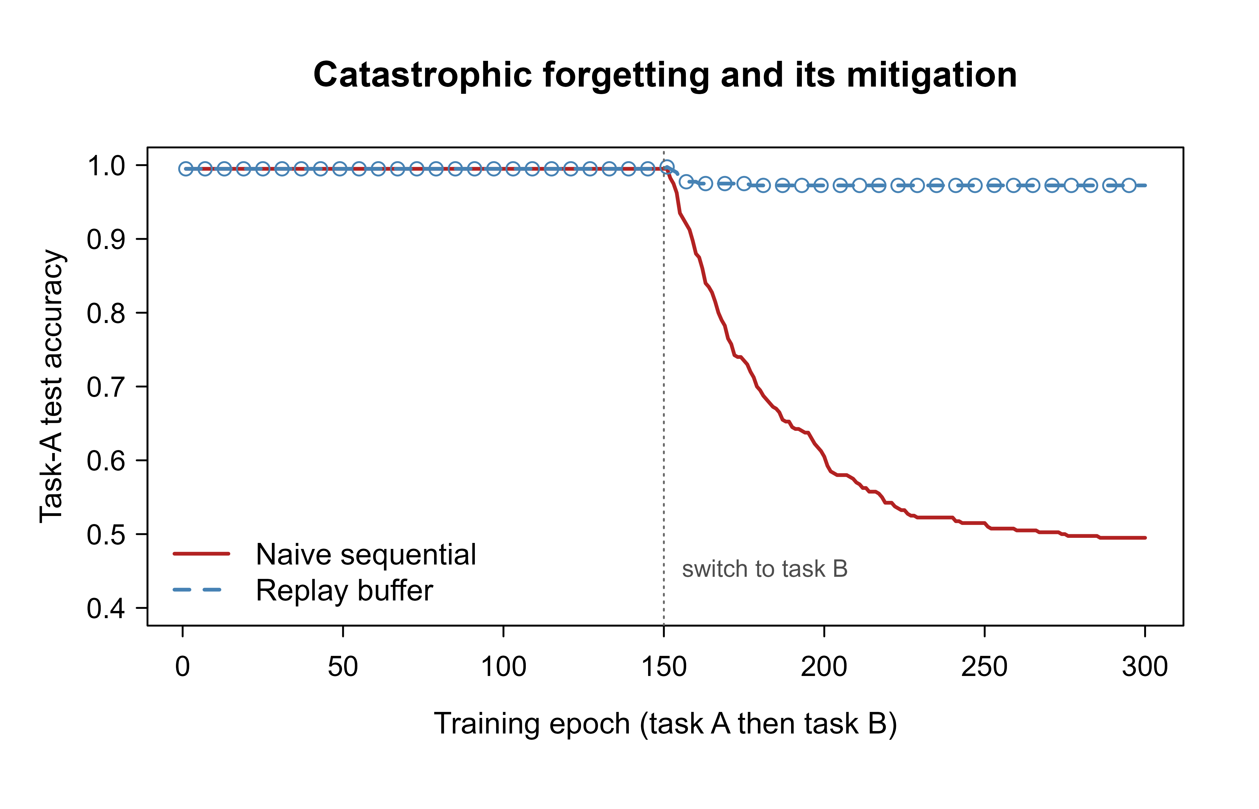
Figure 58.1 is the whole chapter in one picture: a task-blind objective forgets, and a method that keeps even a sliver of the old objective alive does not.
Warning
Do not read the exact accuracy numbers as universal. They depend on the learning rate, the angle between the two tasks, and the buffer size. The robust takeaway is the shape: naive training drops sharply at the task switch, and replay flattens that drop. On harder problems (deep nets, many tasks, class-incremental) the same qualitative gap appears, usually wider.
58.4.6 Verifying the Quadratic Forgetting Law
The claim behind both Equation 58.3 and the EWC penalty is that, near a task-A optimum, the rise in task-A loss caused by a small displacement \(\Delta\) is the quadratic form \(\tfrac12\Delta^\top H_A\Delta\). We can confirm this directly. We train a logistic model on task A to a near-optimum, compute the analytic Hessian of the cross-entropy at that point, then perturb the parameters in random directions and compare the actual loss increase against the quadratic prediction.
Show code
# Cross-entropy loss (no weight decay) on a task, for full param vector c(w, b).
ce_loss <- function(pars, task) {
  par <- list(w = pars[1:2], b = pars[3])
  p <- predict_prob(par, task$X)
  p <- pmin(pmax(p, 1e-12), 1 - 1e-12)
  -mean(task$y * log(p) + (1 - task$y) * log(1 - p))
}

# Train task A to a tight optimum (no decay, so grad -> 0).
parA <- init_par()
for (e in seq_len(4000)) parA <- gd_step(parA, taskA$X, taskA$y, lr = 0.5, wd = 0)
theta_star <- c(parA$w, parA$b)

# Analytic Hessian of mean cross-entropy: (1/n) sum_i p_i(1-p_i) z_i z_i^T,
# with z_i = c(x_i1, x_i2, 1). This is also the (model-label) Fisher here.
Z <- cbind(taskA$X, 1)
p <- predict_prob(parA, taskA$X)
H <- t(Z) %*% (Z * (p * (1 - p))) / nrow(Z)

L0 <- ce_loss(theta_star, taskA)
set.seed(7)
cmp <- t(sapply(1:6, function(k) {
  delta <- 0.05 * rnorm(3)
  actual <- ce_loss(theta_star + delta, taskA) - L0
  quad   <- 0.5 * as.numeric(t(delta) %*% H %*% delta)
  c(actual = actual, quadratic = quad)
}))
round(cmp, 6)
#>        actual quadratic
#> [1,] 0.000003  0.000017
#> [2,] 0.000017  0.000019
#> [3,] 0.000000  0.000003
#> [4,] 0.000104  0.000111
#> [5,] 0.000071  0.000079
#> [6,] 0.000001  0.000006
The two columns agree to several decimals, confirming that the Hessian (equivalently the Fisher, here) predicts the task-A loss increase from a parameter move. EWC simply adds this predicted increase, with the Hessian replaced by its diagonal, as a penalty, so the optimizer is charged for the forgetting that Equation 58.3 says it would otherwise incur.
58.5 Theoretical Properties and Failure Modes
A few results sharpen when each family works and when it breaks.
Geometry of regularization. When task B is itself locally quadratic with optimum \(\theta_B^\star\) and curvature \(H_B\), the EWC objective Equation 58.4 (with task-A penalty matrix \(A = \lambda\,\operatorname{diag}(F)\)) is a sum of two quadratics, whose unique minimizer is the precision-weighted average
\[ \hat\theta = (H_B + A)^{-1}(H_B\,\theta_B^\star + A\,\theta_A^\star). \tag{58.8}\]
This is exactly the posterior mean of a Gaussian-prior, Gaussian-likelihood model, which is the Bayesian reading of EWC: the old task acts as a prior with precision \(A\) and the new task as a likelihood with precision \(H_B\). As \(\lambda\to\infty\), \(\hat\theta\to\theta_A^\star\) (perfect stability, no learning); as \(\lambda\to 0\), \(\hat\theta\to\theta_B^\star\) (full plasticity, full forgetting). The slider is literally the prior-to-likelihood precision ratio, and Equation 58.8 shows the compromise is optimal only to the extent the local-quadratic assumption holds.
Forgetting bound for replay. If at every step the mixed gradient keeps a nonnegative inner product with each past gradient (the GEM constraint Equation 58.7), then to first order no past loss increases along the trajectory, so cumulative forgetting is bounded by the second-order remainder, which scales with the step size and the past-task curvature. This is why small learning rates and balanced replay together control forgetting, and why pure replay with too few buffer points fails: the estimated old gradient \(\nabla\widehat{\mathcal{L}}_j\) is too noisy for the inner-product condition to hold in expectation.
Capacity accounting for isolation. Parameter isolation has zero forgetting by construction but a hard capacity ceiling. Progressive networks add \(O(d_k)\) parameters per task, so total parameters grow like \(\sum_k d_k\), linear in the number of tasks. PackNet holds parameters fixed but allocates a fraction of the remaining free weights to each task; after \(k\) tasks at fraction \(f\) the free capacity is \((1-f)^k\), an exponential decay that sets a practical limit on how many tasks fit. There is no free lunch: a method that never forgets must pay in parameters, and a method with fixed parameters must eventually forget or refuse new tasks.
Common failure modes
EWC fails when (i) the diagonal-Fisher assumption is badly violated (strongly correlated parameters), (ii) tasks are many, so accumulated stiffness in Equation 58.5 kills plasticity, or (iii) the new optimum is far from \(\theta_A^\star\), so the local quadratic in Equation 58.3 is a poor global model. Replay fails when the buffer is too small (variance), class-imbalanced (biased gradient), or replayed so heavily it overfits. Isolation fails when capacity runs out or when tasks are similar enough that sharing would have helped but isolation forbids it.
58.6 EWC in Practice (Reference Implementation)
The demo above used replay because it runs cleanly in base R. For completeness, here is how the EWC penalty from Section 58.3.1 attaches to a deep model in a typical Python/PyTorch workflow. It is shown for reference and is not executed here, since the book’s runnable examples are in R.
Show code
import torch

def estimate_fisher(model, loader, device):
    """Diagonal Fisher: average squared gradient of the log-likelihood."""
    fisher = {n: torch.zeros_like(p) for n, p in model.named_parameters()}
    model.eval()
    for x, y in loader:
        x, y = x.to(device), y.to(device)
        model.zero_grad()
        logp = torch.log_softmax(model(x), dim=1)
        # sample-wise log-likelihood of the (predicted) label
        nll = torch.nn.functional.nll_loss(logp, y)
        nll.backward()
        for n, p in model.named_parameters():
            if p.grad is not None:
                fisher[n] += p.grad.detach() ** 2
    n_batches = len(loader)
    return {n: f / n_batches for n, f in fisher.items()}

def ewc_penalty(model, star_params, fisher, lam):
    """Quadratic spring pulling each parameter toward its old value."""
    loss = 0.0
    for n, p in model.named_parameters():
        loss = loss + (fisher[n] * (p - star_params[n]) ** 2).sum()
    return 0.5 * lam * loss

# After finishing task A: snapshot params and Fisher, then train task B with
#   total_loss = task_B_loss + ewc_penalty(model, star_params, fisher, lam)
The structure mirrors the math exactly: estimate_fisher computes the diagonal \(F_i\) from squared log-likelihood gradients, and ewc_penalty is the \(\tfrac{\lambda}{2}\sum_i F_i (\theta_i - \theta^\star_{A,i})^2\) spring. For many tasks you accumulate Fisher terms (one snapshot per task, or a running sum).
58.7 Practical Guidance and Pitfalls
Choosing a method is mostly about constraints, not accuracy alone.
When to use this
If you can store a little past data and privacy allows it, start with a small replay buffer. It is the simplest strong baseline and usually beats regularization in head-to-head studies. If storing raw data is forbidden (privacy, regulation) or impossible (the stream is enormous), use a regularization method like EWC or generative replay. If you have a small, fixed set of well-separated tasks and ample parameters, parameter isolation gives zero forgetting at the cost of capacity.
A few traps recur often enough to call out:
- Tuning \(\lambda\) in EWC is delicate. Too small and you still forget; too large and the model becomes rigid and cannot learn task B at all. This is the stability-plasticity slider made literal. Validate it on a held-out mix of old and new tasks, not on the new task alone.
- Replay buffers can overfit. A tiny buffer is seen many times, so the model can memorize those specific points rather than the old task. Keep the buffer balanced across classes, refresh it (reservoir sampling), and do not weight it so heavily that it dominates the new task.
- Evaluate on all tasks, every time. The single most common reporting error is showing only current-task accuracy, which hides forgetting completely. Always track the full accuracy matrix \(a_{k,j}\) and report \(\text{ACC}\) and \(\text{BWT}\) together.
- Task boundaries are often unknown. Much of the cleanest theory assumes you know when one task ends and the next begins. Real streams blur this. If boundaries are fuzzy, prefer methods that do not need them (reservoir replay, online importance estimation).
- Class-incremental is harder than it looks. When new classes arrive with no task hint at test time, the model must also calibrate across tasks. A classifier that is individually good on each task can still be badly biased toward the most recent classes. Watch for this bias explicitly.
Note
Continual learning shares a border with online and incremental learning (Chapter 55), transfer learning (Chapter 54), and meta-learning (Chapter 53), but the goal is distinct. Online learning optimizes performance on a moving target and does not especially care about old data; transfer learning moves knowledge from a source to a single target; continual learning insists on doing well on every task it has ever seen, with bounded resources.
58.8 Further Reading
- McCloskey and Cohen (1989) first documented catastrophic interference in connectionist networks, the empirical root of the whole field.
- Grossberg (1987) framed the stability-plasticity dilemma that organizes every method here.
- Kirkpatrick, Pascanu, Rabinowitz, et al. (2017) introduced elastic weight consolidation and the Bayesian/Fisher derivation used above.
- Zenke, Poole, and Ganguli (2017) proposed Synaptic Intelligence, an online importance estimate with the same quadratic penalty.
- Lopez-Paz and Ranzato (2017) defined the accuracy-matrix metrics (average accuracy, backward and forward transfer) and Gradient Episodic Memory, the projected-gradient view of Section 58.3.2.1.
- Schwarz, Czarnecki, Luketina, et al. (2018) introduced online EWC, the running-Fisher variant with memory independent of the number of tasks used in Section 58.3.1.3.
- Shin, Lee, Kim, and Kim (2017) introduced deep generative replay as a data-free rehearsal alternative.
- Rusu, Rabinowitz, Desjardins, et al. (2016) presented progressive neural networks, a canonical parameter-isolation method; Mallya and Lazebnik (2018) gave PackNet.
- Parisi, Kemker, Part, Kanan, and Wermter (2019) survey continual lifelong learning with neural networks and are a good map of the territory.
- De Lange, Aljundi, Masana, et al. (2021) provide a careful empirical comparison of the three method families under matched budgets.
The notation \(a_{k,j}\) follows the matrix-of-accuracies convention of Lopez-Paz and Ranzato (2017), who also defined forward transfer, the effect of past learning on a task before any of its own data is seen.↩︎
Weight decay is standard practice and is the realistic mechanism of forgetting in this linear demo: when task B stops sending a useful signal to \(w_1\), the decay term has nothing to oppose it, so \(w_1\) shrinks toward zero and task A is lost. In deep nets the same drift happens for a different reason (the shared features are repurposed), but the cure is identical.↩︎