Imagine you have spent a week tuning a model. The code is clean, the cross-validation looks healthy, and you ship it. A month later the predictions quietly go bad. After a long hunt you discover the cause: an upstream team changed a date column from "2024-01-31" to "01/31/2024", your parser turned the unrecognized strings into NA, and a third of your training rows silently lost their most informative feature. Nothing crashed. Nothing warned you. The model just got worse.
This is the everyday reality that makes data validation worth a chapter of its own. Models are only as trustworthy as the data feeding them. A model can be correct in every line of code and still produce nonsense if a column silently changed type, a join duplicated rows, or an upstream sensor started emitting -999 for missing readings.1 Data validation is the practice of stating what you expect about a dataset, checking those expectations automatically, and stopping (or alerting) when reality disagrees.
Intuition
Think of validation as a contract you make a dataset sign before you trust it. You write down, in code, what a “good” dataset looks like (which columns, which types, which value ranges), and you refuse to proceed until the data demonstrates that it complies. The point is not to fix bad data automatically; it is to notice bad data before it does damage.
This chapter treats validation as a first-class part of the modeling pipeline, not an afterthought. By the end you will be able to tell a schema check from a constraint check, read any validation report as the same small table of pass/fail counts, write a data contract and enforce it, and choose between the main R tools for the job. We cover schema and constraint checks, the idea of a data contract, the R packages pointblank and validate, and the principle of failing loudly. We close with a runnable base-R validation engine you can drop into any project, plus a small simulation that shows how the choice of tolerance trades sensitivity against false alarms.
This material underpins the modeling work throughout the book: everything you train, tune, and deploy elsewhere assumes the data arriving at the model is what you think it is. Validation is how you earn that assumption.
104.1 Where validation fits in a modern ML/AI workflow
A typical workflow moves data through several stages:
Validation belongs at the boundary between stages, especially right after ingestion and right before training or scoring. The reason is economic: the cost of a defect grows the further downstream it travels. A type mismatch caught at ingestion costs seconds. The same defect caught after a model has been retrained on corrupted data, deployed, and used to make decisions can cost far more, because by then the bad data has propagated into features, model weights, and live decisions.
Key idea
Put a check at every boundary where you stop trusting and start computing. The two boundaries that pay off the most are right after ingestion (the handoff from someone else’s system to yours) and right before training or scoring (the handoff from your data prep to your model).
Why bother encoding these expectations in code at all, rather than relying on a careful analyst to eyeball the data? Three observations make the case.
Data changes more often than code. Upstream teams alter schemas, vendors change file formats, and sensors drift. Code review catches code changes; only automated checks catch data changes.
Silent corruption is the dangerous kind. A pipeline that crashes is annoying but safe. A pipeline that quietly trains on bad data is dangerous because the failure surfaces later as degraded predictions, when the link to the root cause is hard to trace.
The same checks serve training and serving. The expectations you assert about training data are exactly the expectations that must hold at inference time. Reusing them prevents training/serving skew.
In an AI/ML context, validation also guards the inputs to feature stores (Chapter 119) and the outputs of LLM-based extraction steps (Chapter 40), where free text gets parsed into structured fields that may or may not conform to a schema.2
Note
Validation does not replace exploratory data analysis. EDA is how you discover what to expect; validation is how you encode and enforce those expectations so they keep holding on every future batch.
104.2 Schema and constraint checks
Before reaching for any tool, it helps to separate the kinds of expectation you might have into two layers, because they fail for different reasons and call for different responses.
The first layer is the schema check, which concerns the shape of the data: which columns exist, their types, and their order. Schema is structural; it describes the container, not the contents. Examples are “the frame has columns id, age, income, signup_date,” “age is an integer,” and “signup_date is a date.”
The second layer is the constraint check, which concerns the values living inside that shape. Constraints are semantic; they describe what the contents are allowed to be. Examples are “age lies in \([0, 120]\),” “income is non-negative,” “id is unique,” “no more than 2% of income is missing,” and “signup_date is not in the future.”
The distinction is not pedantry, it points straight at the diagnosis. Schema failures usually mean the wrong file or a breaking upstream change: someone renamed a column or shipped a different table entirely. Constraint failures usually mean the right file with bad records: the structure is fine but a sensor went haywire or a data-entry slip crept in. Both matter, and a good validation layer reports them separately so you know which kind of problem you are chasing.
Tip
When a report shows a schema failure, look upstream (wrong source, changed format). When it shows only constraint failures, look at the records (bad values in an otherwise correct file). Conflating the two is the fastest way to waste an afternoon debugging.
104.2.1 A formal view of a validation report
The tools in this chapter look different on the surface (one uses a pipe-friendly “agent,” another stores rules as objects, a third hides inside a modeling recipe), but underneath they all compute the same thing. It is worth writing that thing down once, because once you see it, every report becomes readable.
Intuition
Every check answers one question: “what fraction of the data fails this rule?” That fraction is then compared against a threshold you chose. Pass or fail is just “is the fraction small enough?” Nothing in any of the packages below is more complicated than that, no matter how polished the report looks.
Let the dataset be a table \(D\) with \(n\) rows. A validation suite is an ordered list of checks \(V = (v_1, \dots, v_m)\). Each check \(v_k\) is a predicate applied either to the whole table or row by row. For a row-level check, define the indicator
Setting \(\tau_k = 0\) gives a strict check (any failing row fails the whole check). Setting \(\tau_k > 0\) gives a tolerant check, useful when a small rate of bad records is acceptable but a spike is not. This is the warn/fail threshold idea that pointblank exposes directly.
When to use this
Use \(\tau_k = 0\) for things that must never be wrong, such as primary keys and column types. Use a small positive \(\tau_k\) for messy real-world fields where a few bad rows per batch are normal but a sudden jump means something broke.
The suite as a whole is summarized by an action level. A common rule:
with \(\tau^{\text{warn}}_k \le \tau^{\text{fail}}_k\), so a batch that is bad enough to fail is always at least bad enough to warn. Every package below is, at bottom, computing the \(p_k\) values and comparing them to thresholds. Once you see the report as a table of \((\text{check}, n, f_k, p_k, \text{pass})\) rows, the tools stop looking magical and start looking like spreadsheets.
104.3 Data contracts and failing loudly
So far we have talked about checks in isolation. In a real organization the more useful unit is the data contract: an agreement between a data producer and a data consumer about the schema and constraints the producer promises to deliver. The contract is written down (as code or as a machine-readable spec) and enforced automatically. When the producer breaks the contract, the consumer’s pipeline detects it at the boundary rather than absorbing the damage. The word “contract” is apt because it shifts the burden: instead of the consumer hoping the data is fine, the producer is held to an explicit, testable promise.
Two design principles make a contract worth having rather than just decorative.
The first is fail loudly, fail early. When an expectation is violated in a batch pipeline, the default should be to stop with a clear, actionable error that says which check failed, how badly, and on which rows. A pipeline that swallows validation failures and continues is worse than one with no validation at all, because it manufactures false confidence: people trust output that has not earned it. In R this means letting validation issue stop() for hard failures, not merely printing a message that scrolls past in a log nobody reads.
The second is quarantine, do not silently drop. When a tolerant check fails on a minority of rows, route those rows to a quarantine table for later inspection rather than deleting them. Dropping bad rows hides the existence of a problem and the count keeps looking healthy; quarantining surfaces the problem while letting the good rows proceed.
Warning
Silently dropping rows that fail a check is one of the most common and most damaging anti-patterns in data pipelines. The bug disappears from view but the data is now biased, because the rows you discarded were not a random sample. Always count and store what you remove.
With the principles in place, the practical question is which tool to reach for. The table below contrasts the main R tooling so you can match a tool to a situation; the sections that follow walk through each in turn.
Table 104.1: Comparison of the main R tools for data validation, contrasting their paradigm, report object, threshold handling, and best-fit situation.
Tool
Paradigm
Report object
Thresholds / actions
Best fit
pointblank
Fluent “agent” building a validation plan, then interrogating data
Rich report table (HTML/console), step-by-step
warn/stop/notify at fractional thresholds
Production tables, scheduled checks, shareable reports
Table 104.1 summarizes how the four approaches differ in paradigm, report object, threshold handling, and the situations each suits best. A practical setup uses more than one: pointblank or validate at ingestion for broad coverage and human-readable reports, and recipes checks inside the model pipeline so that serving-time data is validated with the exact rules used at training time.
104.4 The pointblank package
The pointblank package builds a validation plan with a pipe-friendly grammar that reads almost like a checklist. You create an agent that points at a table, add validation steps to it, then call interrogate() to run them all. Each step records its fail fraction \(p_k\) and compares it to thresholds you set with action_levels(), which is exactly the warn/fail machinery from the formal view. The agent then produces a report you can read in a browser or query in code.
When to use this
Reach for pointblank when checks recur (scheduled batches, production tables) and when a human needs to read the result. Its strength is the shareable, step-by-step report.
Because pointblank is not installed in the runnable library used to build this book, the next three chunks are set to eval=FALSE. The code is current and idiomatic, so it will run unchanged once the package is installed.
Show code
library(pointblank)# Define warn/stop thresholds as fractions of failing rows.# warn at 1% failing, stop the pipeline at 5% failing.al<-action_levels(warn_at =0.01, stop_at =0.05)agent<-create_agent( tbl =mtcars, label ="mtcars contract", actions =al)|># schema-style checkscol_exists(columns =c(mpg, cyl, hp, wt))|>col_is_numeric(columns =c(mpg, hp, wt))|># constraint checkscol_vals_gt(columns =mpg, value =0)|>col_vals_between(columns =cyl, left =3, right =12)|>col_vals_not_null(columns =wt)|>rows_distinct()|>interrogate()# Human-readable report (renders as HTML in a browser / RStudio viewer)agent# Programmatic access to the pass/fail decision for CI or a pipeline gateall_passed(agent)# TRUE only if no step exceeded its stop thresholdx<-get_agent_x_list(agent)# list with f_failed, f_passed, etc. per step
That report is for humans. To enforce the contract inside an automated batch job, you want the “fail loudly” principle in action: wrap the agent so that a stop-level breach raises an actual error and halts the run.
Sometimes the full agent is more ceremony than you need, for example inside a function where you just want one quick assertion. For those lightweight inline checks (no agent, immediate result), pointblank offers the test_* and expect_* families, which pair well with the testthat testing framework:
Show code
library(pointblank)# returns TRUE/FALSE, does not stoptest_col_vals_between(mtcars, columns =mpg, left =10, right =35)# stops with an informative condition if violated (good for pipelines)mtcars|>col_vals_gt(columns =hp, value =0)|>col_vals_not_null(columns =mpg)
104.5 The validate package
Where pointblank builds a plan step by step, the validate package takes a declarative stance: you write the rules once, store them as an object (or even in an external YAML or CSV file), and then confront any dataset with them. The shift in mindset is small but powerful: rules become data. You can keep them in version control, hand them to a domain expert to edit, and reuse the same rule set across many projects, all without touching pipeline code.
Intuition
pointblank feels like writing a script (“do this check, then this one”). validate feels like writing a spec sheet (“here are the laws this data must obey”) and then asking, “does this batch obey them?” Both compute the same fail fractions; they differ in how you author and store the rules.
This package is also not in the runnable library here, so the chunk is eval=FALSE.
Show code
library(validate)rules<-validator( mpg_positive =mpg>0, cyl_in_range =in_range(cyl, min =3, max =12), wt_present =!is.na(wt), hp_reasonable =hp<1000)cf<-confront(mtcars, rules)summary(cf)# one row per rule: items, passes, fails, error, warningplot(cf)# bar chart of pass/fail counts per rule
Because rules are objects, you can keep them under version control separately from the data, import them across projects, and let analysts edit them without touching pipeline code. This is the rule-library pattern used in official statistics, where validation rules number in the hundreds.
104.6 Checks inside a tidymodels pipeline
The tools so far validate data as a standalone step. But recall the training/serving skew problem: the surest way to guarantee the model sees consistent data is to validate it with the exact same code at training time and at serving time. The recipes package (part of the tidymodels framework, Chapter 90) makes this automatic. A recipe bundles preprocessing steps into one object, and its check_* steps raise an error during bake() if a rule is violated. Because the very same recipe object that prepared the training data is the one that processes serving data, the contract travels with the pipeline and cannot drift apart from it.
Key idea
Embedding checks in the recipe means there is no separate “did you remember to validate serving data?” step to forget. The recipe refuses to transform data that breaks the contract, so a violation surfaces before a single prediction is made.
The exact arguments accepted by check_range() have shifted across recipes versions, so consult ?check_range for the version you have installed. The shape of the idea is stable even when the argument names move: a check step that errors at bake() time.
All four tools (the agent, the rule object, the recipe step, and the base-R engine we build next) compute the same fail fractions. They differ only in ergonomics and in where the report lands. With the conceptual map in hand, we can now build a working engine from scratch and watch it catch real defects.
104.7 A runnable base-R validation engine
The best way to convince yourself there is no magic is to build the engine yourself. The previous tools share one core: compute a fail fraction per check and compare it to a tolerance. The function below does exactly that in plain base R, with no packages at all. It checks column existence, column type, value ranges, and missingness, and returns a tidy pass/fail report whose columns are the \((\text{check}, n, f_k, p_k, \text{pass})\) tuple from the formal view. This chunk is eval=TRUE and runs as part of building the book.
Tip
Read the function once for shape, not detail. The helper add() appends one report row per check; the loop walks each column in the schema and calls add() for existence, type, missingness, range, and uniqueness. Everything else is bookkeeping.
Show code
# A small data-validation engine in base R.# `data`: a data.frame to validate.# `schema`: a named list; each element describes one column's contract:# type : expected class, one of "numeric","integer","character","factor","Date"# min,max : optional numeric/Date bounds for range checking# max_na : tolerance for the fraction of missing values (default 0)# unique : logical, should the column have no duplicate values (default FALSE)validate_data<-function(data, schema){results<-list()add<-function(check, column, n, fails){p<-if(n>0)fails/nelse0results[[length(results)+1]]<<-data.frame( check =check, column =column, n =n, fails =fails, fail_pct =round(100*p, 2), pass =fails==0, stringsAsFactors =FALSE)}n<-nrow(data)for(colinnames(schema)){# Use [[ ]] for all lookups: $ does partial matching, so spec$max would# silently resolve to spec$max_na. Exact extraction avoids that trap.spec<-schema[[col]]spec_min<-spec[["min"]]spec_max<-spec[["max"]]spec_max_na<-spec[["max_na"]]# 1. existence (schema check)if(!col%in%names(data)){add("exists", col, n, n)# treat all rows as failingnext# cannot run further checks on a missing column}add("exists", col, n, 0)x<-data[[col]]# 2. type (schema check)type_ok<-switch(spec[["type"]], numeric =is.numeric(x), integer =is.integer(x), character =is.character(x), factor =is.factor(x), Date =inherits(x, "Date"),stop("Unknown type in schema: ", spec[["type"]]))add("type", col, n, if(type_ok)0elsen)# 3. missingness (constraint check with tolerance)max_na<-if(is.null(spec_max_na))0elsespec_max_nan_na<-sum(is.na(x))# a missingness "failure" is the excess over the tolerated counttol_count<-floor(max_na*n)add("missing", col, n, max(0, n_na-tol_count))# 4. range (constraint check), only on non-missing comparable valuesif(!is.null(spec_min)||!is.null(spec_max)){xv<-x[!is.na(x)]below<-if(!is.null(spec_min))xv<spec_minelserep(FALSE, length(xv))above<-if(!is.null(spec_max))xv>spec_maxelserep(FALSE, length(xv))add("range", col, n, sum(below|above))}# 5. uniqueness (constraint check)if(isTRUE(spec[["unique"]])){dup<-sum(duplicated(x))add("unique", col, n, dup)}}report<-do.call(rbind, results)rownames(report)<-NULLreport}# A convenience gate that fails loudly when any check fails.assert_valid<-function(data, schema){rep<-validate_data(data, schema)if(!all(rep$pass)){bad<-rep[!rep$pass, c("check", "column", "fail_pct")]msg<-paste0(" - ", bad$check, " on '", bad$column,"' (", bad$fail_pct, "% failing)", collapse ="\n")stop("Data contract violated:\n", msg, call. =FALSE)}invisible(data)}
104.7.1 Demonstration on clean and corrupted data
A function is only convincing once you watch it catch something. So we now build a schema, then run it against a clean frame and a deliberately corrupted copy of it, injecting the kinds of defects that real pipelines suffer so the report shows genuine failures rather than a wall of green.
Show code
set.seed(1)clean<-data.frame( id =1:200, age =sample(18:90, 200, replace =TRUE), income =round(rlnorm(200, meanlog =10, sdlog =0.4)), signup =as.Date("2020-01-01")+sample(0:1000, 200, replace =TRUE))contract<-list( id =list(type ="integer", unique =TRUE), age =list(type ="integer", min =0, max =120), income =list(type ="numeric", min =0, max_na =0.02), signup =list(type ="Date", max =as.Date("2026-01-01")))# Corrupt the data the way real pipelines break:dirty<-cleandirty$age[c(3, 50)]<-c(-5L, 250L)# impossible ages (range)dirty$income[1:20]<-NA# 10% missing, over the 2% tolerancedirty$id[10]<-dirty$id[9]# duplicate primary keydirty$signup[7]<-as.Date("2030-06-01")# future dateclean_report<-validate_data(clean, contract)dirty_report<-validate_data(dirty, contract)clean_report#> check column n fails fail_pct pass#> 1 exists id 200 0 0 TRUE#> 2 type id 200 0 0 TRUE#> 3 missing id 200 0 0 TRUE#> 4 unique id 200 0 0 TRUE#> 5 exists age 200 0 0 TRUE#> 6 type age 200 0 0 TRUE#> 7 missing age 200 0 0 TRUE#> 8 range age 200 0 0 TRUE#> 9 exists income 200 0 0 TRUE#> 10 type income 200 0 0 TRUE#> 11 missing income 200 0 0 TRUE#> 12 range income 200 0 0 TRUE#> 13 exists signup 200 0 0 TRUE#> 14 type signup 200 0 0 TRUE#> 15 missing signup 200 0 0 TRUE#> 16 range signup 200 0 0 TRUEdirty_report#> check column n fails fail_pct pass#> 1 exists id 200 0 0.0 TRUE#> 2 type id 200 0 0.0 TRUE#> 3 missing id 200 0 0.0 TRUE#> 4 unique id 200 1 0.5 FALSE#> 5 exists age 200 0 0.0 TRUE#> 6 type age 200 0 0.0 TRUE#> 7 missing age 200 0 0.0 TRUE#> 8 range age 200 2 1.0 FALSE#> 9 exists income 200 0 0.0 TRUE#> 10 type income 200 0 0.0 TRUE#> 11 missing income 200 16 8.0 FALSE#> 12 range income 200 0 0.0 TRUE#> 13 exists signup 200 0 0.0 TRUE#> 14 type signup 200 0 0.0 TRUE#> 15 missing signup 200 0 0.0 TRUE#> 16 range signup 200 1 0.5 FALSE
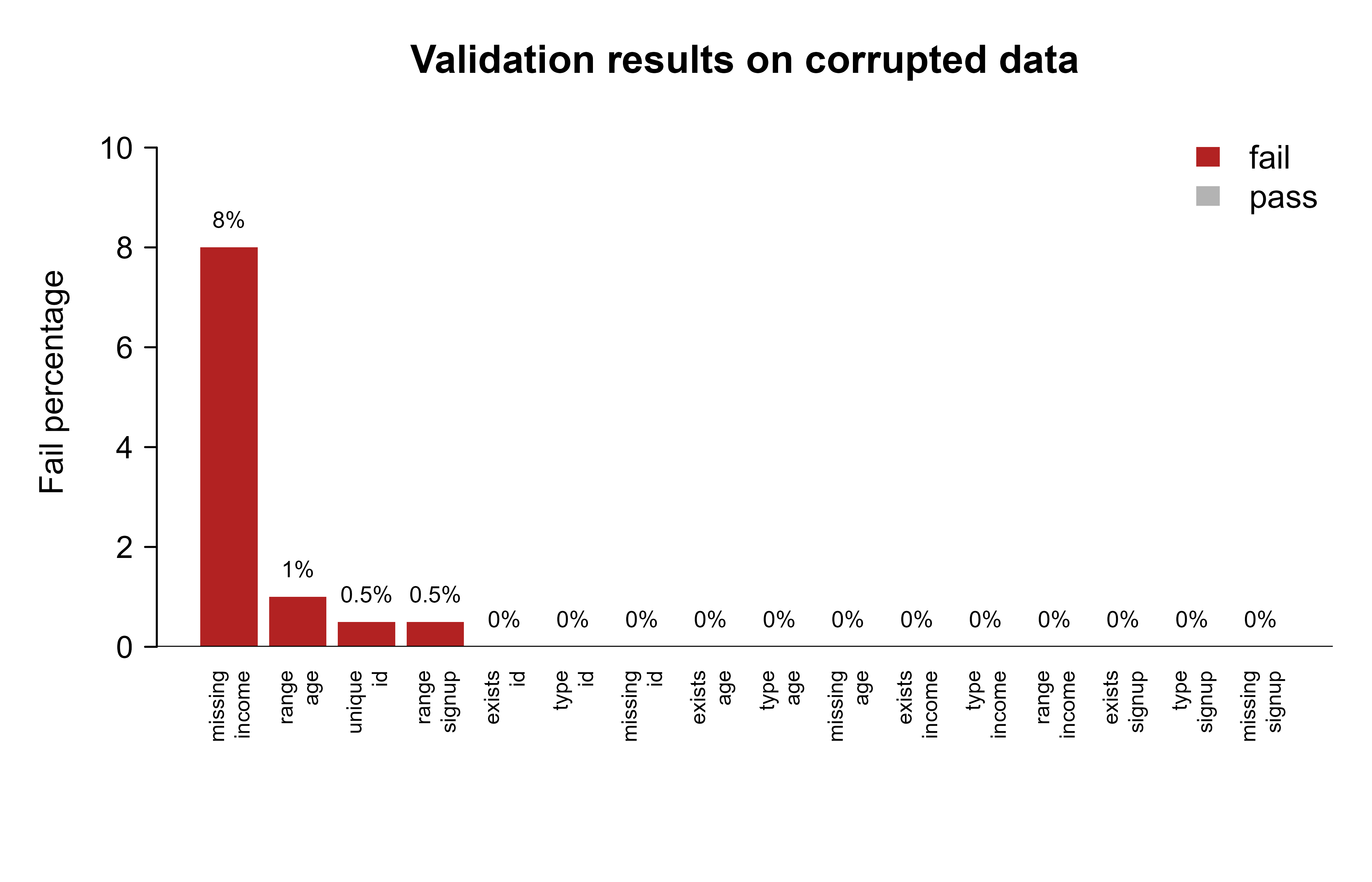
The clean report passes every row, as it should. The dirty report localizes each defect to a (check, column) pair with its fail percentage: the duplicate key shows up under unique on id, the two impossible ages under range on age, the missing incomes under missing on income, and the future date under range on signup. That is precisely the \((k, p_k)\) structure from the formal view, now filled in with real numbers. Notice that the missingness failure (8%) far exceeds the 2% tolerance we set, which is why it is flagged, while a single bad row in a 200-row column registers as just 0.5%.
104.7.2 A figure: fail rates across checks
A report table is precise, but when you are scanning a pipeline at 2 a.m. a chart makes a spike obvious at a glance in a way a column of numbers does not. The next chunk plots the fail percentage of every check on the corrupted data, coloring failures red so they jump out. Figure 104.1 shows the result: every defect we injected appears as a red bar, while the checks that passed sit flat at zero in grey.
Show code
dr<-dirty_reportdr$label<-paste(dr$check, dr$column, sep ="\n")ord<-order(dr$fail_pct, decreasing =TRUE)dr<-dr[ord, ]bar_col<-ifelse(dr$pass, "grey70", "firebrick")op<-par(mar =c(6, 4, 3, 1))bp<-barplot(dr$fail_pct, names.arg =dr$label, col =bar_col, border =NA, ylab ="Fail percentage", main ="Validation results on corrupted data", las =2, cex.names =0.65, ylim =c(0, max(dr$fail_pct)*1.2+1))text(bp, dr$fail_pct, labels =paste0(dr$fail_pct, "%"), pos =3, cex =0.7, xpd =NA)abline(h =0, col ="black")legend("topright", fill =c("firebrick", "grey70"), legend =c("fail", "pass"), bty ="n", border =NA)par(op)
Figure 104.1: Fail percentage per validation check on the corrupted dataset. Bars above zero flag contract violations.
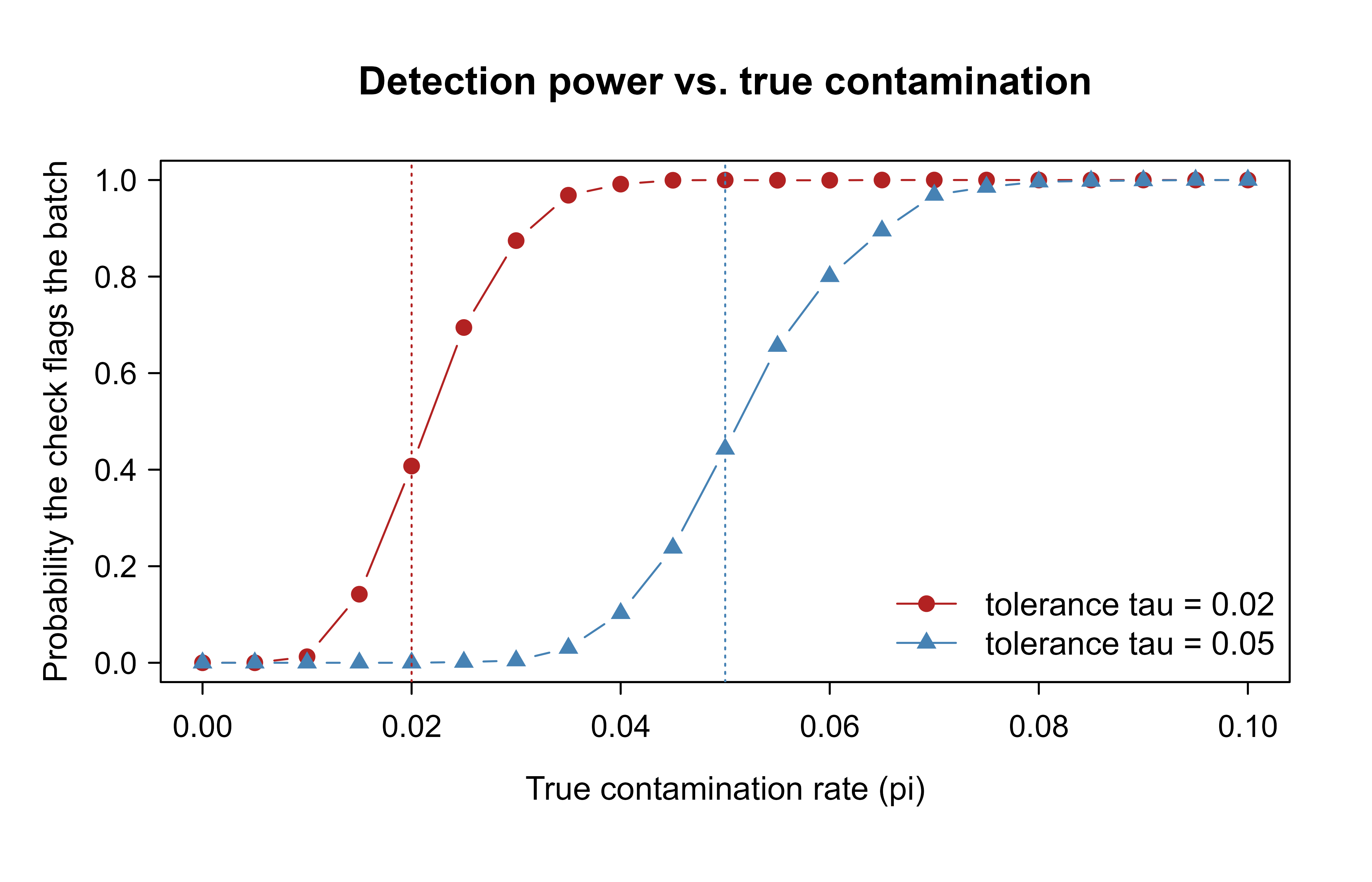
104.7.3 A simulation: detection power under a drifting fail rate
We claimed earlier that the choice of tolerance \(\tau_k\) trades sensitivity against false alarms. That trade-off is easy to assert and easy to get wrong by intuition, so let us measure it. We simulate batches whose true contamination rate \(\pi\) (the actual fraction of bad rows being generated upstream) ranges from 0 to 10%, and we count how often a check with tolerance \(\tau\) raises a failure. Averaged over many simulated batches, that count estimates the detection probability, the chance the check fires given a true contamination rate \(\pi\):
as a function of the true rate \(\pi\), for two tolerances. Here \(B_i\) is the indicator that row \(i\) is contaminated, so the average \(\frac{1}{n}\sum_i B_i\) is the observed fail fraction the check compares to \(\tau\). Figure 104.2 plots the resulting detection probability for a strict and a lenient tolerance.
Show code
set.seed(42)simulate_power<-function(pi, n=500, tau=0.02, reps=2000){flags<-replicate(reps, {bad<-rbinom(1, size =n, prob =pi)# number of contaminated rows(bad/n)>tau# does it breach tolerance?})mean(flags)}pis<-seq(0, 0.10, by =0.005)pow_strict<-sapply(pis, simulate_power, tau =0.02)pow_lenient<-sapply(pis, simulate_power, tau =0.05)plot(pis, pow_strict, type ="b", pch =19, col ="firebrick", xlab ="True contamination rate (pi)", ylab ="Probability the check flags the batch", main ="Detection power vs. true contamination", ylim =c(0, 1))lines(pis, pow_lenient, type ="b", pch =17, col ="steelblue")abline(v =0.02, lty =3, col ="firebrick")abline(v =0.05, lty =3, col ="steelblue")legend("bottomright", legend =c("tolerance tau = 0.02", "tolerance tau = 0.05"), col =c("firebrick", "steelblue"), pch =c(19, 17), lty =1, bty ="n")
Figure 104.2: Probability a tolerant check flags a batch, as the true contamination rate rises. A stricter tolerance detects smaller problems but is more sensitive to noise near the threshold.
Both curves rise from near 0 to near 1 as \(\pi\) crosses the corresponding tolerance, and the shape is the whole story. When the true contamination rate sits below \(\tau\), any flag is a false alarm caused by sampling noise, and the strict check (red) raises more of these because its threshold is closer to the noise. When the true rate climbs above \(\tau\), the check reliably fires, and the strict check gets there sooner, catching smaller problems. So choosing \(\tau\) is choosing where you want the transition to sit, which in turn depends on how much a missed problem costs you versus how much a false alarm costs you.
Warning
A tolerance set too tight cries wolf. If a check fails on noise every other run, people learn to ignore it, and then it stays ignored on the day it finally matters. An alert that is routinely overridden is no better than no alert at all.
104.8 Practical guidance, pitfalls, and when to use it
Having seen the machinery, the harder question is how to use it well in practice. The advice below distills the habits that separate validation that protects you from validation that merely decorates a pipeline.
When to validate. Always validate at ingestion (the trust boundary with upstream) and immediately before training or scoring. For high-stakes pipelines, validate outputs too: predictions outside a plausible range often signal an input problem, and continuous checks of this kind connect directly to model monitoring (Chapter 117).
Set tolerances deliberately. A tolerance of 0 is right for keys and types, which should never be wrong. Small positive tolerances suit noisy real-world fields where a few bad records are normal but a spike is not. Tie the tolerance to a cost, not to a round number that feels safe.
Separate schema from constraints in reporting. A schema failure usually means “wrong or broken file”; a constraint failure usually means “right file, bad rows.” Conflating them slows diagnosis.
Fail loudly for hard checks, quarantine for soft ones. Hard violations (type, missing key) should stop(). Soft violations should route offending rows to a quarantine table and continue with the rest, so good data is not held hostage by a few bad records.
Validate the same way at train and serve. Reusing the training-time contract at inference is the single most effective guard against training/serving skew. recipescheck_* steps make this automatic.
Common pitfalls. A handful of mistakes recur often enough to be worth naming explicitly, so you can recognize them before they bite:
Validating after cleaning instead of before. By then you have already masked the defect; you want to see the raw problem.
Checking only marginal properties. Many real defects are relational: duplicated join keys, broken foreign keys, row counts that drop by half. Add cross-column and cross-table checks, not just per-column ranges.
Treating NA, empty string, and sentinel values (-999, 9999) as distinct when upstream uses them interchangeably for “missing.” Normalize sentinels before missingness checks, or the missingness check will pass while data is in fact absent.
Letting reports scroll past in logs. A report nobody reads is not validation. Gate the pipeline on the result, or route it to an alert.
Over-tight tolerances that cry wolf. If a check fails on noise every other run, people start ignoring it, and then it fails to fire when it matters.
When not to use heavy tooling. For a one-off exploratory analysis, a handful of stopifnot() calls is enough, and reaching for a full validation framework would be over-engineering. The investment in pointblank or validate pays off when data recurs (scheduled batches, retraining, production scoring), where the same expectations must hold every time and the report must be shareable.
To pull the chapter together: validation is the act of writing down what you expect of a dataset and refusing to proceed when reality disagrees. Every tool reduces to the same calculation, the fail fraction \(p_k\) compared against a tolerance \(\tau_k\), so the skill is less about any one package and more about choosing good expectations, setting tolerances against real costs, failing loudly on hard violations, and quarantining rather than hiding the soft ones. Do that at the trust boundaries of your pipeline, with the same rules at training and serving, and the models in the rest of this book get to assume the one thing they most need: that the data is what you think it is.
104.9 Further reading
Wickham, H., & Grolemund, G. (2017). R for Data Science. O’Reilly. Chapters on import and tidy data motivate why structural expectations matter.
van der Loo, M., & de Jonge, E. (2018). Statistical Data Cleaning with Applications in R. Wiley. The reference for the validate and errorlocate approach to rules-as-data.
Iannone, R., & Vargas, M. (2023). pointblank: Data Quality Assessment and Metadata Reporting for Data Frames and Database Tables. Package documentation and articles.
Schelter, S., Lange, D., Schmidt, P., Celikel, M., Biessmann, F., & Grafberger, A. (2018). Automating large-scale data quality verification. Proceedings of the VLDB Endowment. Describes the Deequ system and the constraint/metric model that inspired modern data-quality tooling.
Polyzotis, N., Roy, S., Whang, S. E., & Zinkevich, M. (2017). Data management challenges in production machine learning. ACM SIGMOD. On validation and training/serving skew in ML systems.
Breck, E., Polyzotis, N., Roy, S., Whang, S. E., & Zinkevich, M. (2019). Data validation for machine learning. Proceedings of MLSys. The data-contract and schema-drift perspective for ML pipelines.
A sentinel value is a special in-band code that stands in for “no measurement,” such as -999, 9999, or an empty string. It is dangerous precisely because it is a valid number: arithmetic and type checks accept it, so it slips past naive checks while corrupting every average and model that touches it.↩︎
A feature store is a shared repository of computed model inputs reused across teams and projects. Training/serving skew is the situation where the data a model sees in production differs systematically from the data it was trained on; validating both with the same rules is one of the most reliable defenses against it.↩︎
Source Code
# Data Validation and Quality {#sec-data-validation}```{r}#| include: falsesource("_common.R")```Imagine you have spent a week tuning a model. The code is clean, the cross-validation looks healthy, and you ship it. A month later the predictions quietly go bad. After a long hunt you discover the cause: an upstream team changed a date column from `"2024-01-31"` to `"01/31/2024"`, your parser turned the unrecognized strings into `NA`, and a third of your training rows silently lost their most informative feature. Nothing crashed. Nothing warned you. The model just got worse.This is the everyday reality that makes data validation worth a chapter of its own. Models are only as trustworthy as the data feeding them. A model can be correct in every line of code and still produce nonsense if a column silently changed type, a join duplicated rows, or an upstream sensor started emitting `-999` for missing readings.^[A *sentinel value* is a special in-band code that stands in for "no measurement," such as `-999`, `9999`, or an empty string. It is dangerous precisely because it is a valid number: arithmetic and type checks accept it, so it slips past naive checks while corrupting every average and model that touches it.] Data validation is the practice of stating what you expect about a dataset, checking those expectations automatically, and stopping (or alerting) when reality disagrees.::: {.callout-tip title="Intuition"}Think of validation as a contract you make a dataset sign before you trust it. You write down, in code, what a "good" dataset looks like (which columns, which types, which value ranges), and you refuse to proceed until the data demonstrates that it complies. The point is not to fix bad data automatically; it is to *notice* bad data before it does damage.:::This chapter treats validation as a first-class part of the modeling pipeline, not an afterthought. By the end you will be able to tell a schema check from a constraint check, read any validation report as the same small table of pass/fail counts, write a data contract and enforce it, and choose between the main R tools for the job. We cover schema and constraint checks, the idea of a data contract, the R packages `pointblank` and `validate`, and the principle of failing loudly. We close with a runnable base-R validation engine you can drop into any project, plus a small simulation that shows how the choice of tolerance trades sensitivity against false alarms.This material underpins the modeling work throughout the book: everything you train, tune, and deploy elsewhere assumes the data arriving at the model is what you think it is. Validation is how you earn that assumption.## Where validation fits in a modern ML/AI workflowA typical workflow moves data through several stages:```ingest -> validate -> clean/transform -> feature engineering -> train -> evaluate -> deploy -> monitor```Validation belongs at the boundary between stages, especially right after ingestion and right before training or scoring. The reason is economic: the cost of a defect grows the further downstream it travels. A type mismatch caught at ingestion costs seconds. The same defect caught after a model has been retrained on corrupted data, deployed, and used to make decisions can cost far more, because by then the bad data has propagated into features, model weights, and live decisions.::: {.callout-important title="Key idea"}Put a check at every boundary where you stop trusting and start computing. The two boundaries that pay off the most are right after ingestion (the handoff from someone else's system to yours) and right before training or scoring (the handoff from your data prep to your model).:::Why bother encoding these expectations in code at all, rather than relying on a careful analyst to eyeball the data? Three observations make the case.1. Data changes more often than code. Upstream teams alter schemas, vendors change file formats, and sensors drift. Code review catches code changes; only automated checks catch data changes.2. Silent corruption is the dangerous kind. A pipeline that crashes is annoying but safe. A pipeline that quietly trains on bad data is dangerous because the failure surfaces later as degraded predictions, when the link to the root cause is hard to trace.3. The same checks serve training and serving. The expectations you assert about training data are exactly the expectations that must hold at inference time. Reusing them prevents training/serving skew.In an AI/ML context, validation also guards the inputs to feature stores (@sec-feature-stores) and the outputs of LLM-based extraction steps (@sec-llms), where free text gets parsed into structured fields that may or may not conform to a schema.^[A *feature store* is a shared repository of computed model inputs reused across teams and projects. *Training/serving skew* is the situation where the data a model sees in production differs systematically from the data it was trained on; validating both with the same rules is one of the most reliable defenses against it.]::: {.callout-note}Validation does not replace exploratory data analysis. EDA is how you *discover* what to expect; validation is how you *encode and enforce* those expectations so they keep holding on every future batch.:::## Schema and constraint checksBefore reaching for any tool, it helps to separate the kinds of expectation you might have into two layers, because they fail for different reasons and call for different responses.The first layer is the schema check, which concerns the shape of the data: which columns exist, their types, and their order. Schema is structural; it describes the container, not the contents. Examples are "the frame has columns `id`, `age`, `income`, `signup_date`," "`age` is an integer," and "`signup_date` is a date."The second layer is the constraint check, which concerns the values living inside that shape. Constraints are semantic; they describe what the contents are allowed to be. Examples are "`age` lies in $[0, 120]$," "`income` is non-negative," "`id` is unique," "no more than 2% of `income` is missing," and "`signup_date` is not in the future."The distinction is not pedantry, it points straight at the diagnosis. Schema failures usually mean the wrong file or a breaking upstream change: someone renamed a column or shipped a different table entirely. Constraint failures usually mean the right file with bad records: the structure is fine but a sensor went haywire or a data-entry slip crept in. Both matter, and a good validation layer reports them separately so you know which kind of problem you are chasing.::: {.callout-tip}When a report shows a schema failure, look upstream (wrong source, changed format). When it shows only constraint failures, look at the records (bad values in an otherwise correct file). Conflating the two is the fastest way to waste an afternoon debugging.:::### A formal view of a validation reportThe tools in this chapter look different on the surface (one uses a pipe-friendly "agent," another stores rules as objects, a third hides inside a modeling recipe), but underneath they all compute the same thing. It is worth writing that thing down once, because once you see it, every report becomes readable.::: {.callout-tip title="Intuition"}Every check answers one question: "what fraction of the data fails this rule?" That fraction is then compared against a threshold you chose. Pass or fail is just "is the fraction small enough?" Nothing in any of the packages below is more complicated than that, no matter how polished the report looks.:::Let the dataset be a table $D$ with $n$ rows. A validation suite is an ordered list of checks $V = (v_1, \dots, v_m)$. Each check $v_k$ is a predicate applied either to the whole table or row by row. For a row-level check, define the indicator$$\mathbf{1}_{k,i} =\begin{cases}1 & \text{if row } i \text{ satisfies check } k \\0 & \text{otherwise}\end{cases}$$The number of failing units for check $k$ is$$f_k = \sum_{i=1}^{n} \big(1 - \mathbf{1}_{k,i}\big),$$and the fail fraction is$$p_k = \frac{f_k}{n}, \qquad p_k \in [0, 1].$$A check passes when $p_k$ is at or below a tolerance $\tau_k \in [0,1]$:$$\text{pass}_k = \big[\, p_k \le \tau_k \,\big].$$Setting $\tau_k = 0$ gives a strict check (any failing row fails the whole check). Setting $\tau_k > 0$ gives a tolerant check, useful when a small rate of bad records is acceptable but a spike is not. This is the warn/fail threshold idea that `pointblank` exposes directly.::: {.callout-tip title="When to use this"}Use $\tau_k = 0$ for things that must never be wrong, such as primary keys and column types. Use a small positive $\tau_k$ for messy real-world fields where a few bad rows per batch are normal but a sudden jump means something broke.:::The suite as a whole is summarized by an action level. A common rule:$$\text{action} =\begin{cases}\texttt{fail} & \text{if } \exists\, k: p_k > \tau^{\text{fail}}_k \\\texttt{warn} & \text{else if } \exists\, k: p_k > \tau^{\text{warn}}_k \\\texttt{pass} & \text{otherwise}\end{cases}$$with $\tau^{\text{warn}}_k \le \tau^{\text{fail}}_k$, so a batch that is bad enough to fail is always at least bad enough to warn. Every package below is, at bottom, computing the $p_k$ values and comparing them to thresholds. Once you see the report as a table of $(\text{check}, n, f_k, p_k, \text{pass})$ rows, the tools stop looking magical and start looking like spreadsheets.## Data contracts and failing loudlySo far we have talked about checks in isolation. In a real organization the more useful unit is the data contract: an agreement between a data producer and a data consumer about the schema and constraints the producer promises to deliver. The contract is written down (as code or as a machine-readable spec) and enforced automatically. When the producer breaks the contract, the consumer's pipeline detects it at the boundary rather than absorbing the damage. The word "contract" is apt because it shifts the burden: instead of the consumer hoping the data is fine, the producer is held to an explicit, testable promise.Two design principles make a contract worth having rather than just decorative.The first is fail loudly, fail early. When an expectation is violated in a batch pipeline, the default should be to stop with a clear, actionable error that says which check failed, how badly, and on which rows. A pipeline that swallows validation failures and continues is worse than one with no validation at all, because it manufactures false confidence: people trust output that has not earned it. In R this means letting validation issue `stop()` for hard failures, not merely printing a message that scrolls past in a log nobody reads.The second is quarantine, do not silently drop. When a tolerant check fails on a minority of rows, route those rows to a quarantine table for later inspection rather than deleting them. Dropping bad rows hides the existence of a problem and the count keeps looking healthy; quarantining surfaces the problem while letting the good rows proceed.::: {.callout-warning}Silently dropping rows that fail a check is one of the most common and most damaging anti-patterns in data pipelines. The bug disappears from view but the data is now biased, because the rows you discarded were not a random sample. Always count and store what you remove.:::With the principles in place, the practical question is which tool to reach for. The table below contrasts the main R tooling so you can match a tool to a situation; the sections that follow walk through each in turn.| Tool | Paradigm | Report object | Thresholds / actions | Best fit ||---|---|---|---|---||`pointblank`| Fluent "agent" building a validation plan, then interrogating data | Rich report table (HTML/console), step-by-step |`warn`/`stop`/`notify` at fractional thresholds | Production tables, scheduled checks, shareable reports ||`validate`| Declarative rules object evaluated against data |`confrontation` object, `summary()` to a data frame | Pass/fail per rule, custom severities | Rules as data, rule libraries, official statistics ||`recipes` (`check_*`) | Checks embedded in a modeling preprocessing pipeline | Error at `bake()`/`prep()` time | Hard stop on violation | Guarding train/serve preprocessing in tidymodels || Base R function (this chapter) | Hand-written predicate loop | A plain data frame report | Whatever you code | Teaching the idea, zero-dependency environments |: Comparison of the main R tools for data validation, contrasting their paradigm, report object, threshold handling, and best-fit situation. {#tbl-data-validation-tool-comparison}@tbl-data-validation-tool-comparison summarizes how the four approaches differ in paradigm, report object, threshold handling, and the situations each suits best. A practical setup uses more than one: `pointblank` or `validate` at ingestion for broad coverage and human-readable reports, and `recipes` checks inside the model pipeline so that serving-time data is validated with the exact rules used at training time.## The `pointblank` packageThe `pointblank` package builds a validation plan with a pipe-friendly grammar that reads almost like a checklist. You create an *agent* that points at a table, add validation steps to it, then call `interrogate()` to run them all. Each step records its fail fraction $p_k$ and compares it to thresholds you set with `action_levels()`, which is exactly the warn/fail machinery from the formal view. The agent then produces a report you can read in a browser or query in code.::: {.callout-tip title="When to use this"}Reach for `pointblank` when checks recur (scheduled batches, production tables) and when a human needs to read the result. Its strength is the shareable, step-by-step report.:::Because `pointblank` is not installed in the runnable library used to build this book, the next three chunks are set to `eval=FALSE`. The code is current and idiomatic, so it will run unchanged once the package is installed.```{r pointblank-demo, eval=FALSE}library(pointblank)# Define warn/stop thresholds as fractions of failing rows.# warn at 1% failing, stop the pipeline at 5% failing.al <-action_levels(warn_at =0.01, stop_at =0.05)agent <-create_agent(tbl = mtcars,label ="mtcars contract",actions = al ) |># schema-style checkscol_exists(columns =c(mpg, cyl, hp, wt)) |>col_is_numeric(columns =c(mpg, hp, wt)) |># constraint checkscol_vals_gt(columns = mpg, value =0) |>col_vals_between(columns = cyl, left =3, right =12) |>col_vals_not_null(columns = wt) |>rows_distinct() |>interrogate()# Human-readable report (renders as HTML in a browser / RStudio viewer)agent# Programmatic access to the pass/fail decision for CI or a pipeline gateall_passed(agent) # TRUE only if no step exceeded its stop thresholdx <-get_agent_x_list(agent) # list with f_failed, f_passed, etc. per step```That report is for humans. To enforce the contract inside an automated batch job, you want the "fail loudly" principle in action: wrap the agent so that a stop-level breach raises an actual error and halts the run.```{r pointblank-gate, eval=FALSE}library(pointblank)validate_or_die <-function(tbl) { agent <-create_agent(tbl, actions =action_levels(stop_at =0.001)) |>col_vals_not_null(columns =everything()) |>interrogate()if (!all_passed(agent)) {stop("Data contract violated. See report.", call. =FALSE) }invisible(tbl)}```Sometimes the full agent is more ceremony than you need, for example inside a function where you just want one quick assertion. For those lightweight inline checks (no agent, immediate result), `pointblank` offers the `test_*` and `expect_*` families, which pair well with the `testthat` testing framework:```{r pointblank-inline, eval=FALSE}library(pointblank)# returns TRUE/FALSE, does not stoptest_col_vals_between(mtcars, columns = mpg, left =10, right =35)# stops with an informative condition if violated (good for pipelines)mtcars |>col_vals_gt(columns = hp, value =0) |>col_vals_not_null(columns = mpg)```## The `validate` packageWhere `pointblank` builds a plan step by step, the `validate` package takes a declarative stance: you write the rules once, store them as an object (or even in an external YAML or CSV file), and then *confront* any dataset with them. The shift in mindset is small but powerful: rules become data. You can keep them in version control, hand them to a domain expert to edit, and reuse the same rule set across many projects, all without touching pipeline code.::: {.callout-tip title="Intuition"}`pointblank` feels like writing a script ("do this check, then this one"). `validate` feels like writing a spec sheet ("here are the laws this data must obey") and then asking, "does this batch obey them?" Both compute the same fail fractions; they differ in how you author and store the rules.:::This package is also not in the runnable library here, so the chunk is `eval=FALSE`.```{r validate-demo, eval=FALSE}library(validate)rules <-validator(mpg_positive = mpg >0,cyl_in_range =in_range(cyl, min =3, max =12),wt_present =!is.na(wt),hp_reasonable = hp <1000)cf <-confront(mtcars, rules)summary(cf) # one row per rule: items, passes, fails, error, warningplot(cf) # bar chart of pass/fail counts per rule```Because rules are objects, you can keep them under version control separately from the data, import them across projects, and let analysts edit them without touching pipeline code. This is the rule-library pattern used in official statistics, where validation rules number in the hundreds.## Checks inside a tidymodels pipelineThe tools so far validate data as a standalone step. But recall the training/serving skew problem: the surest way to guarantee the model sees consistent data is to validate it with the *exact same code* at training time and at serving time. The `recipes` package (part of the tidymodels framework, @sec-tidymodels-framework) makes this automatic. A recipe bundles preprocessing steps into one object, and its `check_*` steps raise an error during `bake()` if a rule is violated. Because the very same recipe object that prepared the training data is the one that processes serving data, the contract travels with the pipeline and cannot drift apart from it.::: {.callout-important title="Key idea"}Embedding checks in the recipe means there is no separate "did you remember to validate serving data?" step to forget. The recipe refuses to transform data that breaks the contract, so a violation surfaces before a single prediction is made.:::```{r recipes-check, eval=FALSE}library(recipes)rec <-recipe(mpg ~ ., data = mtcars) |>check_missing(all_predictors()) |># error if any NA appearscheck_range(hp, min =0, max =1000) |># error if hp leaves rangestep_normalize(all_numeric_predictors())prepped <-prep(rec, training = mtcars)# At serving time, baking new data runs the checks before transforming:bake(prepped, new_data = mtcars)```::: {.callout-note}The exact arguments accepted by `check_range()` have shifted across `recipes` versions, so consult `?check_range` for the version you have installed. The shape of the idea is stable even when the argument names move: a check step that errors at `bake()` time.:::All four tools (the agent, the rule object, the recipe step, and the base-R engine we build next) compute the same fail fractions. They differ only in ergonomics and in where the report lands. With the conceptual map in hand, we can now build a working engine from scratch and watch it catch real defects.## A runnable base-R validation engineThe best way to convince yourself there is no magic is to build the engine yourself. The previous tools share one core: compute a fail fraction per check and compare it to a tolerance. The function below does exactly that in plain base R, with no packages at all. It checks column existence, column type, value ranges, and missingness, and returns a tidy pass/fail report whose columns are the $(\text{check}, n, f_k, p_k, \text{pass})$ tuple from the formal view. This chunk is `eval=TRUE` and runs as part of building the book.::: {.callout-tip}Read the function once for shape, not detail. The helper `add()` appends one report row per check; the loop walks each column in the schema and calls `add()` for existence, type, missingness, range, and uniqueness. Everything else is bookkeeping.:::```{r base-engine}# A small data-validation engine in base R.# `data`: a data.frame to validate.# `schema`: a named list; each element describes one column's contract:# type : expected class, one of "numeric","integer","character","factor","Date"# min,max : optional numeric/Date bounds for range checking# max_na : tolerance for the fraction of missing values (default 0)# unique : logical, should the column have no duplicate values (default FALSE)validate_data <-function(data, schema) { results <-list() add <-function(check, column, n, fails) { p <-if (n >0) fails / n else0 results[[length(results) +1]] <<-data.frame(check = check,column = column,n = n,fails = fails,fail_pct =round(100* p, 2),pass = fails ==0,stringsAsFactors =FALSE ) } n <-nrow(data)for (col innames(schema)) {# Use [[ ]] for all lookups: $ does partial matching, so spec$max would# silently resolve to spec$max_na. Exact extraction avoids that trap. spec <- schema[[col]] spec_min <- spec[["min"]] spec_max <- spec[["max"]] spec_max_na <- spec[["max_na"]]# 1. existence (schema check)if (!col %in%names(data)) {add("exists", col, n, n) # treat all rows as failingnext# cannot run further checks on a missing column }add("exists", col, n, 0) x <- data[[col]]# 2. type (schema check) type_ok <-switch( spec[["type"]],numeric =is.numeric(x),integer =is.integer(x),character =is.character(x),factor =is.factor(x),Date =inherits(x, "Date"),stop("Unknown type in schema: ", spec[["type"]]) )add("type", col, n, if (type_ok) 0else n)# 3. missingness (constraint check with tolerance) max_na <-if (is.null(spec_max_na)) 0else spec_max_na n_na <-sum(is.na(x))# a missingness "failure" is the excess over the tolerated count tol_count <-floor(max_na * n)add("missing", col, n, max(0, n_na - tol_count))# 4. range (constraint check), only on non-missing comparable valuesif (!is.null(spec_min) ||!is.null(spec_max)) { xv <- x[!is.na(x)] below <-if (!is.null(spec_min)) xv < spec_min elserep(FALSE, length(xv)) above <-if (!is.null(spec_max)) xv > spec_max elserep(FALSE, length(xv))add("range", col, n, sum(below | above)) }# 5. uniqueness (constraint check)if (isTRUE(spec[["unique"]])) { dup <-sum(duplicated(x))add("unique", col, n, dup) } } report <-do.call(rbind, results)rownames(report) <-NULL report}# A convenience gate that fails loudly when any check fails.assert_valid <-function(data, schema) { rep <-validate_data(data, schema)if (!all(rep$pass)) { bad <- rep[!rep$pass, c("check", "column", "fail_pct")] msg <-paste0(" - ", bad$check, " on '", bad$column,"' (", bad$fail_pct, "% failing)", collapse ="\n")stop("Data contract violated:\n", msg, call. =FALSE) }invisible(data)}```### Demonstration on clean and corrupted dataA function is only convincing once you watch it catch something. So we now build a schema, then run it against a clean frame and a deliberately corrupted copy of it, injecting the kinds of defects that real pipelines suffer so the report shows genuine failures rather than a wall of green.```{r base-demo}set.seed(1)clean <-data.frame(id =1:200,age =sample(18:90, 200, replace =TRUE),income =round(rlnorm(200, meanlog =10, sdlog =0.4)),signup =as.Date("2020-01-01") +sample(0:1000, 200, replace =TRUE))contract <-list(id =list(type ="integer", unique =TRUE),age =list(type ="integer", min =0, max =120),income =list(type ="numeric", min =0, max_na =0.02),signup =list(type ="Date", max =as.Date("2026-01-01")))# Corrupt the data the way real pipelines break:dirty <- cleandirty$age[c(3, 50)] <-c(-5L, 250L) # impossible ages (range)dirty$income[1:20] <-NA# 10% missing, over the 2% tolerancedirty$id[10] <- dirty$id[9] # duplicate primary keydirty$signup[7] <-as.Date("2030-06-01")# future dateclean_report <-validate_data(clean, contract)dirty_report <-validate_data(dirty, contract)clean_reportdirty_report```The clean report passes every row, as it should. The dirty report localizes each defect to a `(check, column)` pair with its fail percentage: the duplicate key shows up under `unique` on `id`, the two impossible ages under `range` on `age`, the missing incomes under `missing` on `income`, and the future date under `range` on `signup`. That is precisely the $(k, p_k)$ structure from the formal view, now filled in with real numbers. Notice that the missingness failure (8%) far exceeds the 2% tolerance we set, which is why it is flagged, while a single bad row in a 200-row column registers as just 0.5%.### A figure: fail rates across checksA report table is precise, but when you are scanning a pipeline at 2 a.m. a chart makes a spike obvious at a glance in a way a column of numbers does not. The next chunk plots the fail percentage of every check on the corrupted data, coloring failures red so they jump out. @fig-data-validation-fail-rates shows the result: every defect we injected appears as a red bar, while the checks that passed sit flat at zero in grey.```{r fig-data-validation-fail-rates, fig.cap="Fail percentage per validation check on the corrupted dataset. Bars above zero flag contract violations.", fig.width=7, fig.height=4.5}dr <- dirty_reportdr$label <-paste(dr$check, dr$column, sep ="\n")ord <-order(dr$fail_pct, decreasing =TRUE)dr <- dr[ord, ]bar_col <-ifelse(dr$pass, "grey70", "firebrick")op <-par(mar =c(6, 4, 3, 1))bp <-barplot( dr$fail_pct,names.arg = dr$label,col = bar_col,border =NA,ylab ="Fail percentage",main ="Validation results on corrupted data",las =2,cex.names =0.65,ylim =c(0, max(dr$fail_pct) *1.2+1))text(bp, dr$fail_pct, labels =paste0(dr$fail_pct, "%"),pos =3, cex =0.7, xpd =NA)abline(h =0, col ="black")legend("topright", fill =c("firebrick", "grey70"),legend =c("fail", "pass"), bty ="n", border =NA)par(op)```### A simulation: detection power under a drifting fail rateWe claimed earlier that the choice of tolerance $\tau_k$ trades sensitivity against false alarms. That trade-off is easy to assert and easy to get wrong by intuition, so let us measure it. We simulate batches whose true contamination rate $\pi$ (the actual fraction of bad rows being generated upstream) ranges from 0 to 10%, and we count how often a check with tolerance $\tau$ raises a failure. Averaged over many simulated batches, that count estimates the *detection probability*, the chance the check fires given a true contamination rate $\pi$:$$\Pr(\text{flag} \mid \pi) = \Pr\!\left(\frac{1}{n}\sum_{i=1}^n B_i > \tau\right), \qquad B_i \sim \text{Bernoulli}(\pi),$$as a function of the true rate $\pi$, for two tolerances. Here $B_i$ is the indicator that row $i$ is contaminated, so the average $\frac{1}{n}\sum_i B_i$ is the observed fail fraction the check compares to $\tau$. @fig-data-validation-detection-power plots the resulting detection probability for a strict and a lenient tolerance.```{r fig-data-validation-detection-power, fig.cap="Probability a tolerant check flags a batch, as the true contamination rate rises. A stricter tolerance detects smaller problems but is more sensitive to noise near the threshold.", fig.width=7, fig.height=4.5}set.seed(42)simulate_power <-function(pi, n =500, tau =0.02, reps =2000) { flags <-replicate(reps, { bad <-rbinom(1, size = n, prob = pi) # number of contaminated rows (bad / n) > tau # does it breach tolerance? })mean(flags)}pis <-seq(0, 0.10, by =0.005)pow_strict <-sapply(pis, simulate_power, tau =0.02)pow_lenient <-sapply(pis, simulate_power, tau =0.05)plot(pis, pow_strict, type ="b", pch =19, col ="firebrick",xlab ="True contamination rate (pi)",ylab ="Probability the check flags the batch",main ="Detection power vs. true contamination",ylim =c(0, 1))lines(pis, pow_lenient, type ="b", pch =17, col ="steelblue")abline(v =0.02, lty =3, col ="firebrick")abline(v =0.05, lty =3, col ="steelblue")legend("bottomright",legend =c("tolerance tau = 0.02", "tolerance tau = 0.05"),col =c("firebrick", "steelblue"), pch =c(19, 17), lty =1, bty ="n")```Both curves rise from near 0 to near 1 as $\pi$ crosses the corresponding tolerance, and the shape is the whole story. When the true contamination rate sits below $\tau$, any flag is a false alarm caused by sampling noise, and the strict check (red) raises more of these because its threshold is closer to the noise. When the true rate climbs above $\tau$, the check reliably fires, and the strict check gets there sooner, catching smaller problems. So choosing $\tau$ is choosing where you want the transition to sit, which in turn depends on how much a missed problem costs you versus how much a false alarm costs you.::: {.callout-warning}A tolerance set too tight cries wolf. If a check fails on noise every other run, people learn to ignore it, and then it stays ignored on the day it finally matters. An alert that is routinely overridden is no better than no alert at all.:::## Practical guidance, pitfalls, and when to use itHaving seen the machinery, the harder question is how to use it well in practice. The advice below distills the habits that separate validation that protects you from validation that merely decorates a pipeline.When to validate. Always validate at ingestion (the trust boundary with upstream) and immediately before training or scoring. For high-stakes pipelines, validate outputs too: predictions outside a plausible range often signal an input problem, and continuous checks of this kind connect directly to model monitoring (@sec-model-monitoring).Set tolerances deliberately. A tolerance of 0 is right for keys and types, which should never be wrong. Small positive tolerances suit noisy real-world fields where a few bad records are normal but a spike is not. Tie the tolerance to a cost, not to a round number that feels safe.Separate schema from constraints in reporting. A schema failure usually means "wrong or broken file"; a constraint failure usually means "right file, bad rows." Conflating them slows diagnosis.Fail loudly for hard checks, quarantine for soft ones. Hard violations (type, missing key) should `stop()`. Soft violations should route offending rows to a quarantine table and continue with the rest, so good data is not held hostage by a few bad records.Validate the same way at train and serve. Reusing the training-time contract at inference is the single most effective guard against training/serving skew. `recipes``check_*` steps make this automatic.Common pitfalls. A handful of mistakes recur often enough to be worth naming explicitly, so you can recognize them before they bite:- Validating after cleaning instead of before. By then you have already masked the defect; you want to see the raw problem.- Checking only marginal properties. Many real defects are relational: duplicated join keys, broken foreign keys, row counts that drop by half. Add cross-column and cross-table checks, not just per-column ranges.- Treating `NA`, empty string, and sentinel values (`-999`, `9999`) as distinct when upstream uses them interchangeably for "missing." Normalize sentinels before missingness checks, or the missingness check will pass while data is in fact absent.- Letting reports scroll past in logs. A report nobody reads is not validation. Gate the pipeline on the result, or route it to an alert.- Over-tight tolerances that cry wolf. If a check fails on noise every other run, people start ignoring it, and then it fails to fire when it matters.When not to use heavy tooling. For a one-off exploratory analysis, a handful of `stopifnot()` calls is enough, and reaching for a full validation framework would be over-engineering. The investment in `pointblank` or `validate` pays off when data recurs (scheduled batches, retraining, production scoring), where the same expectations must hold every time and the report must be shareable.To pull the chapter together: validation is the act of writing down what you expect of a dataset and refusing to proceed when reality disagrees. Every tool reduces to the same calculation, the fail fraction $p_k$ compared against a tolerance $\tau_k$, so the skill is less about any one package and more about choosing good expectations, setting tolerances against real costs, failing loudly on hard violations, and quarantining rather than hiding the soft ones. Do that at the trust boundaries of your pipeline, with the same rules at training and serving, and the models in the rest of this book get to assume the one thing they most need: that the data is what you think it is.## Further reading- Wickham, H., & Grolemund, G. (2017). *R for Data Science.* O'Reilly. Chapters on import and tidy data motivate why structural expectations matter.- van der Loo, M., & de Jonge, E. (2018). *Statistical Data Cleaning with Applications in R.* Wiley. The reference for the `validate` and `errorlocate` approach to rules-as-data.- Iannone, R., & Vargas, M. (2023). *pointblank: Data Quality Assessment and Metadata Reporting for Data Frames and Database Tables.* Package documentation and articles.- Schelter, S., Lange, D., Schmidt, P., Celikel, M., Biessmann, F., & Grafberger, A. (2018). Automating large-scale data quality verification. *Proceedings of the VLDB Endowment.* Describes the Deequ system and the constraint/metric model that inspired modern data-quality tooling.- Polyzotis, N., Roy, S., Whang, S. E., & Zinkevich, M. (2017). Data management challenges in production machine learning. *ACM SIGMOD.* On validation and training/serving skew in ML systems.- Breck, E., Polyzotis, N., Roy, S., Whang, S. E., & Zinkevich, M. (2019). Data validation for machine learning. *Proceedings of MLSys.* The data-contract and schema-drift perspective for ML pipelines.