| Property | Vanilla RNN | LSTM | GRU |
|---|---|---|---|
| States carried | h_t | h_t and c_t | h_t |
| Number of gates | 0 | 3 (f, i, o) | 2 (z, r) |
| Long-memory path | none | additive cell state | convex blend |
| Gradient factor | D_i W_h (uncontrolled) | diag(f_i) (learned) | diag(1 - z_i) (learned) |
| Relative parameters | 1x | ~4x | ~3x |
37 Recurrent Neural Networks: LSTMs and GRUs
Most of the models in this book treat each observation as a fixed bundle of features with no inherent order. A row is a row, and shuffling the rows changes nothing. Sequences break that assumption. A sentence is not a bag of words, a patient’s chart is not a bag of lab values, and a stock price today depends on where it was yesterday. The order carries the meaning, and a model that ignores order throws away exactly the signal we care about.
Recurrent neural networks (RNNs) are the classical neural answer to this. The idea is almost embarrassingly simple: read the sequence one step at a time, and carry a running summary of everything seen so far. That summary, the hidden state, is updated at each step by the same small network, so the model has a kind of memory that it reuses across positions. A feedforward network (Chapter 15) sees the whole input at once; an RNN sees it as a story unfolding in time.
The simplicity hides a serious difficulty. Carrying memory across many steps means multiplying many derivatives together when we train, and products of many numbers either collapse to zero or explode to infinity. This is the vanishing and exploding gradient problem, and it is the reason vanilla RNNs struggle to learn dependencies that span more than a handful of steps. The long short-term memory (LSTM) cell and the gated recurrent unit (GRU) were engineered specifically to keep a gradient alive across long spans, and they did so well enough to power machine translation, speech recognition, and time series forecasting for the better part of a decade before attention and Transformers (Chapter 38) took over.
This chapter builds the recurrence from intuition to mechanism. We define the vanilla RNN precisely, derive backpropagation through time and the exact condition under which its gradients vanish or explode, then show how the gating in LSTMs and GRUs creates an additive path that lets gradients survive. We close with sequence-to-sequence modelling, guidance on when to reach for a Transformer instead, and a runnable base-R demonstration of an RNN forward pass together with a numerical illustration of gradient vanishing.
Key idea
An RNN applies the same update at every time step and threads a hidden state through the sequence. Sharing the update is what lets the model generalize across positions; threading the state is what gives it memory. Both come at the cost of a long multiplicative chain in the gradient.
37.1 The Recurrence
Let the input be a sequence of vectors \(x_1, x_2, \dots, x_T\), with each \(x_t \in \mathbb{R}^{d}\). An RNN maintains a hidden state \(h_t \in \mathbb{R}^{m}\) that summarizes the prefix \(x_1, \dots, x_t\). The defining equation is the recurrence
\[ h_t = f(h_{t-1}, x_t), \tag{37.1}\]
with \(h_0\) a fixed or learned initial state (often the zero vector). The same function \(f\) is applied at every step, which is the parameter sharing that distinguishes an RNN from simply stacking \(T\) separate layers.
The classic “Elman” choice for \(f\) is an affine map followed by a squashing nonlinearity,
\[ h_t = \tanh\!\big(W_{h} h_{t-1} + W_{x} x_t + b_h\big), \tag{37.2}\]
where \(W_h \in \mathbb{R}^{m \times m}\), \(W_x \in \mathbb{R}^{m \times d}\), and \(b_h \in \mathbb{R}^{m}\) are shared across all time steps. Each step produces an output through a read-out layer applied to the hidden state,
\[ \hat{y}_t = g\!\big(W_{y} h_t + b_y\big), \tag{37.3}\]
where \(g\) is the identity for regression or a softmax for classification over a vocabulary. Depending on the task we use the output at every step (for example, tagging each word), only the final output \(\hat{y}_T\) (for example, classifying a whole review), or a separate decoder (for sequence-to-sequence, below).
Note
Unrolling the recurrence over \(T\) steps gives a feedforward network that is \(T\) layers deep but with every layer tied to the same weights. This “unrolled” view is what makes ordinary backpropagation applicable, and it is also where the depth, and hence the gradient trouble, comes from.
The number of parameters does not grow with \(T\): it is \(m(m + d) + m\) for the recurrent layer plus the read-out, regardless of how long the sequence is. The computational cost of a forward pass is \(O(T m^2)\) for the hidden updates, and because each \(h_t\) needs \(h_{t-1}\), the steps must run in sequence and cannot be parallelized along the time axis. That serial dependency is one of the practical reasons Transformers eventually displaced RNNs.
37.2 Backpropagation Through Time
Training minimizes a loss summed over time,
\[ \mathcal{L} = \sum_{t=1}^{T} \mathcal{L}_t(\hat{y}_t, y_t), \tag{37.4}\]
with respect to the shared parameters \(\theta = \{W_h, W_x, b_h, W_y, b_y\}\). Because the same weights appear at every step, the gradient with respect to, say, \(W_h\) collects contributions from all steps. Backpropagation through time (BPTT) is ordinary backpropagation applied to the unrolled graph, with one twist: gradients that flow into the shared weights are accumulated across all the time steps at which those weights were used.
37.2.1 Deriving the gradient
Write the pre-activation at step \(t\) as \(a_t = W_h h_{t-1} + W_x x_t + b_h\), so that \(h_t = \tanh(a_t)\). We want \(\partial \mathcal{L} / \partial W_h\). By the chain rule, summing over the steps where \(W_h\) acts,
\[ \frac{\partial \mathcal{L}}{\partial W_h} = \sum_{t=1}^{T} \frac{\partial \mathcal{L}_t}{\partial h_t}\, \frac{\partial h_t}{\partial W_h}\Bigg|_{\text{total}}, \tag{37.5}\]
where the “total” derivative of \(h_t\) with respect to \(W_h\) must account for the fact that \(h_t\) depends on \(W_h\) both directly and through every earlier \(h_k\). Unrolling that dependence, the loss at a single step \(t\) sends gradient back to every earlier step \(k \le t\) along the chain of hidden states. The contribution of step \(t\) to the gradient of the hidden state at step \(k\) is
\[ \frac{\partial \mathcal{L}_t}{\partial h_k} = \frac{\partial \mathcal{L}_t}{\partial h_t}\, \frac{\partial h_t}{\partial h_k}, \qquad k \le t, \tag{37.6}\]
and the crucial factor is the Jacobian product that carries the signal from step \(t\) back to step \(k\),
\[ \frac{\partial h_t}{\partial h_k} = \prod_{i=k+1}^{t} \frac{\partial h_i}{\partial h_{i-1}}. \tag{37.7}\]
Each factor in this product is the per-step Jacobian. Differentiating Equation 37.2,
\[ \frac{\partial h_i}{\partial h_{i-1}} = D_i \, W_h, \qquad D_i = \operatorname{diag}\!\big(1 - \tanh^2(a_i)\big), \tag{37.8}\]
where \(D_i\) is the diagonal matrix of \(\tanh'\) values, each entry in \((0, 1]\). Substituting Equation 37.8 into Equation 37.7 shows that carrying gradient across \(t - k\) steps means multiplying \(t - k\) copies of \(D_i W_h\) together. The behaviour of that long product is the whole story.
37.2.2 The vanishing and exploding gradient
Take norms of the Jacobian product in Equation 37.7. By submultiplicativity,
\[ \left\| \frac{\partial h_t}{\partial h_k} \right\| \le \prod_{i=k+1}^{t} \| D_i \, W_h \| \le \prod_{i=k+1}^{t} \| D_i \| \, \| W_h \|. \tag{37.9}\]
Since every diagonal entry of \(D_i\) lies in \((0, 1]\) for the \(\tanh\) activation, \(\|D_i\| \le 1\) in the spectral norm, so the entire product is bounded by \(\|W_h\|^{\,t-k}\). Let \(\gamma = \|W_h\|\) (equivalently its largest singular value, and closely related to its largest eigenvalue \(\lambda_{\max}\)). Then
\[ \left\| \frac{\partial h_t}{\partial h_k} \right\| \lesssim \gamma^{\,t-k}. \tag{37.10}\]
The consequences are immediate and sharp:
- If \(\gamma < 1\), the gradient norm decays geometrically as the gap \(t - k\) grows. A signal from 50 steps back is multiplied by \(\gamma^{50}\), which for \(\gamma = 0.9\) is about \(0.005\). The early steps receive essentially no learning signal. This is the vanishing gradient problem.
- If \(\gamma > 1\), the same product grows geometrically and the gradient explodes, producing wild updates and numerical overflow.
A more precise statement uses the eigendecomposition. If \(W_h = V \Lambda V^{-1}\) with eigenvalues \(\lambda_j\), then the repeated product is dominated by \(\lambda_{\max}^{\,t-k}\). The borderline case \(\lambda_{\max} = 1\) is the only one that neither vanishes nor explodes, and it is measure-zero in practice, so a generic deep recurrence sits on one side of the knife edge or the other.
Warning
The diagonal factor \(D_i\) makes things worse, not better, for vanishing. Because \(\tanh' = 1 - \tanh^2 \le 1\) and is strictly below \(1\) whenever the unit is even slightly saturated, the realized decay is usually faster than the \(\gamma^{t-k}\) bound suggests. Saturated \(\tanh\) units kill the gradient on their own.
Exploding gradients have a cheap practical fix: gradient clipping, where the gradient vector is rescaled to a maximum norm before each update,
\[ \tilde{g} = g \cdot \frac{\min(\tau, \|g\|)}{\|g\|}, \tag{37.11}\]
for a threshold \(\tau\). This caps the explosion without changing the gradient’s direction. Vanishing gradients are the harder problem, because there is no information left to rescale once it has decayed. Solving vanishing required changing the architecture itself, which is what gating does.
37.3 The LSTM Cell
The LSTM (Hochreiter and Schmidhuber, 1997) introduces a second state, the cell state \(c_t\), that runs along the sequence with a nearly linear update. Where the vanilla hidden state is transformed by a full nonlinear map at every step, the cell state is mostly added to, and addition has a gradient of one. Three learned gates, each a sigmoid-squashed linear function of the input and previous hidden state, decide what to erase, what to write, and what to read out.
Writing \(\sigma\) for the logistic sigmoid and \(\odot\) for elementwise product, the LSTM computes, at each step,
\[ \begin{aligned} f_t &= \sigma\!\big(W_f [h_{t-1}, x_t] + b_f\big), \\ i_t &= \sigma\!\big(W_i [h_{t-1}, x_t] + b_i\big), \\ o_t &= \sigma\!\big(W_o [h_{t-1}, x_t] + b_o\big), \\ \tilde{c}_t &= \tanh\!\big(W_c [h_{t-1}, x_t] + b_c\big), \end{aligned} \tag{37.12}\]
where \([h_{t-1}, x_t]\) denotes concatenation. The forget gate \(f_t\), input gate \(i_t\), and output gate \(o_t\) all take values in \((0,1)\) per coordinate. The state updates are then
\[ c_t = f_t \odot c_{t-1} + i_t \odot \tilde{c}_t, \qquad h_t = o_t \odot \tanh(c_t). \tag{37.13}\]
The cell update in Equation 37.13 is the heart of the design. The previous cell \(c_{t-1}\) is scaled by the forget gate and then a new candidate is added in. When the forget gate is near one and the input gate near zero, the cell simply copies itself forward: \(c_t \approx c_{t-1}\). That is a near-identity path along the time axis, sometimes called the constant error carousel.
37.3.1 Why gating preserves gradients
Repeat the Jacobian argument from Equation 37.7, but now along the cell state. The relevant per-step derivative is \(\partial c_t / \partial c_{t-1}\). From the cell update, treating the gates as approximately constant over the path (they depend on \(h_{t-1}\), but the dominant term is explicit),
\[ \frac{\partial c_t}{\partial c_{t-1}} \approx \operatorname{diag}(f_t). \tag{37.14}\]
The product that carries gradient from step \(t\) back to step \(k\) is therefore approximately
\[ \frac{\partial c_t}{\partial c_k} \approx \prod_{i=k+1}^{t} \operatorname{diag}(f_i) = \operatorname{diag}\!\left( \prod_{i=k+1}^{t} f_i \right). \tag{37.15}\]
Compare this with the vanilla product \(\prod_i D_i W_h\) in Equation 37.7. Two things have changed. First, there is no repeated multiplication by a weight matrix \(W_h\), so the eigenvalues of \(W_h\) no longer drive the decay. Second, the multiplicative factors are the forget gates \(f_i \in (0,1)\), which the network learns to set. If a unit needs to remember something for a long time, gradient descent can push the relevant forget gates toward one, making \(\prod_i f_i \approx 1\) and keeping the gradient alive across the whole span.
The vanilla RNN had no such control: its decay rate \(\gamma = \|W_h\|\) is a single number shared by all paths and all time scales. The LSTM makes the per-step memory coefficient a learned, input-dependent gate, so different units can remember over different horizons. This is precisely why initializing the forget-gate bias \(b_f\) to a positive value (so gates start near one) is a standard and effective trick: it starts the network in a “remember by default” regime.
Tip
The intuition that “addition has gradient one” is the same one behind residual connections in very deep feedforward networks and behind the skip path in Transformers. Whenever you see an additive update \(z_t = z_{t-1} + (\text{something})\), expect a clean gradient highway through it.
37.4 The GRU
The gated recurrent unit (Cho et al., 2014) is a streamlined gating scheme. It drops the separate cell state and uses only two gates, an update gate \(z_t\) and a reset gate \(r_t\):
\[ \begin{aligned} z_t &= \sigma\!\big(W_z [h_{t-1}, x_t] + b_z\big), \\ r_t &= \sigma\!\big(W_r [h_{t-1}, x_t] + b_r\big), \\ \tilde{h}_t &= \tanh\!\big(W_h [\, r_t \odot h_{t-1}, \, x_t \,] + b_h\big), \end{aligned} \tag{37.16}\]
with the hidden state formed as a convex blend of the old state and the candidate,
\[ h_t = (1 - z_t) \odot h_{t-1} + z_t \odot \tilde{h}_t. \tag{37.17}\]
The update gate \(z_t\) plays the combined role of the LSTM’s forget and input gates: when \(z_t \approx 0\) the state is copied forward unchanged, giving the same near-identity path and the same gradient-preserving product \(\prod_i (1 - z_i)\) as in Equation 37.15. The reset gate \(r_t\) controls how much of the past enters the candidate, letting the unit “forget” the prior state when computing a fresh proposal.
A GRU has fewer parameters than an LSTM (three weight blocks rather than four) and is faster to train. Empirically the two perform comparably on most tasks; LSTMs sometimes have an edge on very long dependencies because the separate cell state gives them an extra degree of freedom, while GRUs are often preferred when data or compute is limited. There is no universal winner, and the choice is usually settled by validation performance.
37.5 Sequence to Sequence and When to Prefer Transformers
Many tasks map one sequence to another of a different length: translating a sentence, summarizing a paragraph, transcribing speech. The classic RNN solution is the encoder-decoder architecture. An encoder RNN reads the input \(x_1, \dots, x_T\) and compresses it into its final hidden state \(h_T\), the context vector. A decoder RNN is then initialized from that context and generates the output \(y_1, \dots, y_{T'}\) one token at a time, feeding each predicted token back in as the next input,
\[ s_t = f_{\text{dec}}(s_{t-1}, y_{t-1}), \qquad s_0 = h_T. \tag{37.18}\]
The weakness is the bottleneck: the entire input must be squeezed through the single fixed-size vector \(h_T\), and for long inputs the early content is lost (the same vanishing problem, now framed as forgetting). The historical fix was attention, which lets the decoder look back at all of the encoder’s hidden states rather than just the last one. Attention proved so effective that it was eventually used without recurrence at all, giving the Transformer (Chapter 38).
When should you still reach for an RNN? The honest answer in modern practice is: rarely for large-scale language, where Transformers dominate, but RNNs remain a sensible default in a few situations.
- Streaming or online inference. An RNN processes one step at a time with constant memory, which suits real-time signals (sensors, audio) where you cannot wait for the whole sequence.
- Short sequences and small data. With limited data, the smaller parameter count of a GRU can generalize better than a data-hungry Transformer.
- Strict latency or memory budgets. Self-attention costs \(O(T^2)\) in time and memory; an RNN is \(O(T)\). For very long sequences on constrained hardware, that difference matters.
Prefer a Transformer when you have long-range dependencies, enough data to feed it, and hardware that rewards parallelism, which is to say most modern problems at scale. The connection to probabilistic sequence models such as those in Chapter 77 is worth keeping in mind: an RNN with a softmax read-out is a learned autoregressive factorization of \(p(y_1, \dots, y_T)\), just with a neural parameterization of each conditional.
Note
Bidirectional RNNs run one recurrence forward and another backward, then concatenate the two hidden states, so each position sees both past and future context. They are useful for tagging and classification where the whole sequence is available at once, but not for streaming generation, where the future is unknown.
37.6 A Worked Demonstration in R
We now make two things concrete in base R: the forward pass of a vanilla RNN, and the numerical reality of vanishing gradients across many steps. No deep learning library is needed; the recurrence is a short loop over matrix multiplications.
The first chunk runs a vanilla RNN forward over a random sequence and then measures how the magnitude of the backpropagated gradient changes as we increase the number of steps. We do this for two recurrent weight matrices, one scaled to have spectral radius below one (vanishing) and one above one (exploding), to show both regimes predicted by Equation 37.10.
Show code
set.seed(1)

m <- 8                          # hidden dimension
T_max <- 60                     # maximum number of steps

# A recurrent matrix with a prescribed gain: scale a random orthogonal matrix,
# so its spectral norm and spectral radius both equal `gain` exactly.
make_W <- function(m, gain) {
  Q <- qr.Q(qr(matrix(rnorm(m * m), m, m)))
  gain * Q
}

# Linearized backprop through time: with tanh' = 1 the Jacobian dh_T/dh_0 is the
# matrix product W^steps (eq-rnn-jacprod); we report its spectral norm. The
# linearization isolates the gain of W from the forward-pass saturation that, in
# a real tanh RNN, keeps every tanh' <= 1 and can therefore damp explosion.
grad_norm_through_time <- function(W, steps) {
  J <- diag(nrow(W))
  for (t in seq_len(steps)) J <- W %*% J
  norm(J, type = "2")
}

W_vanish  <- make_W(m, 0.7)
W_explode <- make_W(m, 1.3)

steps_grid <- seq(2, T_max, by = 2)
g_vanish  <- sapply(steps_grid, function(s) grad_norm_through_time(W_vanish,  s))
g_explode <- sapply(steps_grid, function(s) grad_norm_through_time(W_explode, s))

df <- rbind(
  data.frame(steps = steps_grid, gnorm = g_vanish,  regime = "gain 0.7"),
  data.frame(steps = steps_grid, gnorm = g_explode, regime = "gain 1.3")
)
bound <- rbind(
  data.frame(steps = steps_grid, gnorm = 0.7^steps_grid, regime = "gain 0.7"),
  data.frame(steps = steps_grid, gnorm = 1.3^steps_grid, regime = "gain 1.3")
)

library(ggplot2)
ggplot(df, aes(steps, gnorm, colour = regime)) +
  geom_line() +
  geom_point(size = 1.2) +
  geom_line(data = bound, aes(steps, gnorm, colour = regime),
            linetype = "dashed", linewidth = 0.5) +
  scale_y_log10() +
  labs(x = "number of recurrent steps (t - k)",
       y = "gradient norm  (log scale)",
       colour = NULL,
       title = "Vanishing and exploding gradients in a vanilla RNN") +
  scale_colour_viridis_d(end = 0.7)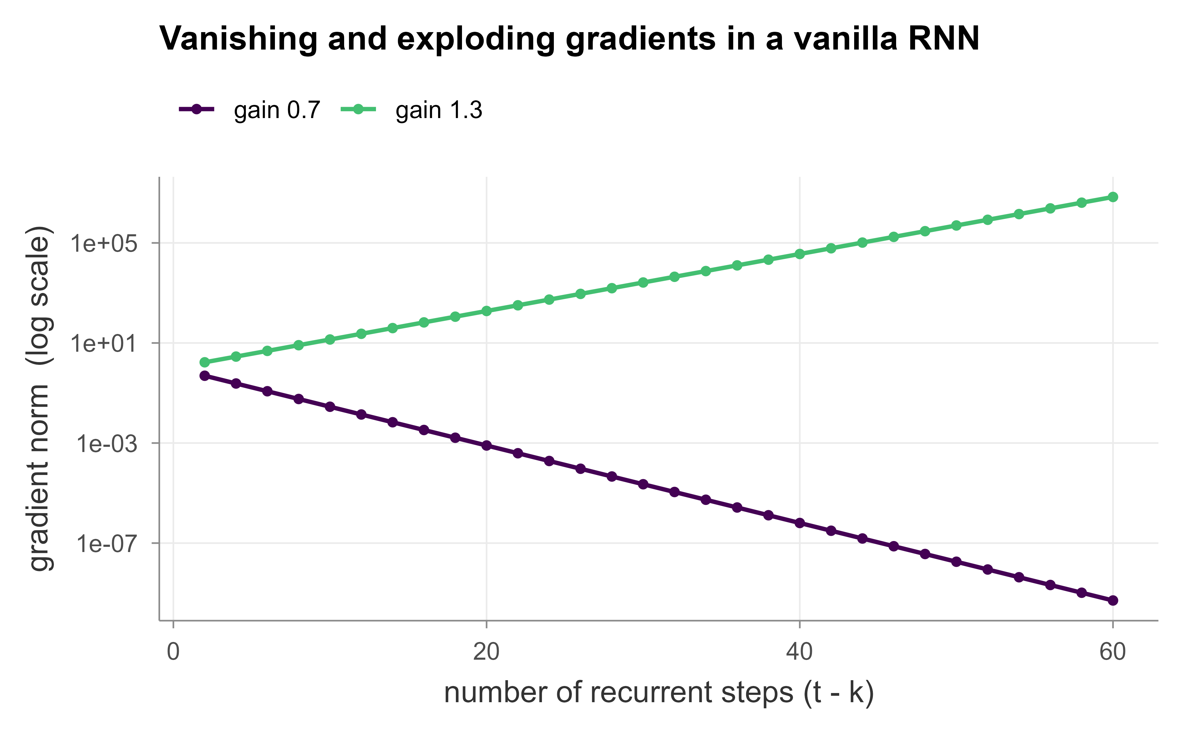
The measured gradient norms (solid) sit exactly on the \(\gamma^{t-k}\) reference (dashed): below one they collapse toward machine zero, and above one they grow by many orders of magnitude over sixty steps. This is Equation 37.10 made visible. With the bounded tanh nonlinearity each factor \(\operatorname{diag}(1 - \tanh^2)\) has spectral norm at most one, so in a real forward pass saturation can damp the explosion (exploding gradients are most acute with unbounded activations), while vanishing remains the dominant tanh failure mode that gating was invented to cure.
The second chunk contrasts the per-step gradient factor of a vanilla RNN with that of an LSTM-style cell, showing how a forget gate near one keeps the cumulative product from decaying.
Show code
set.seed(7)
steps <- 1:60

# Vanilla: product of spectral radius (0.7) per step.
vanilla_factor <- 0.7^steps

# Gated: product of forget gates, each drawn close to one.
forget_gates <- plogis(rnorm(60, mean = 3, sd = 0.3))   # sigmoid of large bias
gated_factor <- cumprod(forget_gates)

dfg <- rbind(
  data.frame(steps = steps, factor = vanilla_factor, cell = "vanilla RNN (radius 0.7)"),
  data.frame(steps = steps, factor = gated_factor,   cell = "gated cell (forget ~ 0.95)")
)

ggplot(dfg, aes(steps, factor, colour = cell)) +
  geom_line() +
  scale_y_log10() +
  labs(x = "number of steps back in time",
       y = "cumulative gradient factor (log scale)",
       colour = NULL,
       title = "Gating preserves the gradient across long spans") +
  scale_colour_viridis_d(end = 0.7)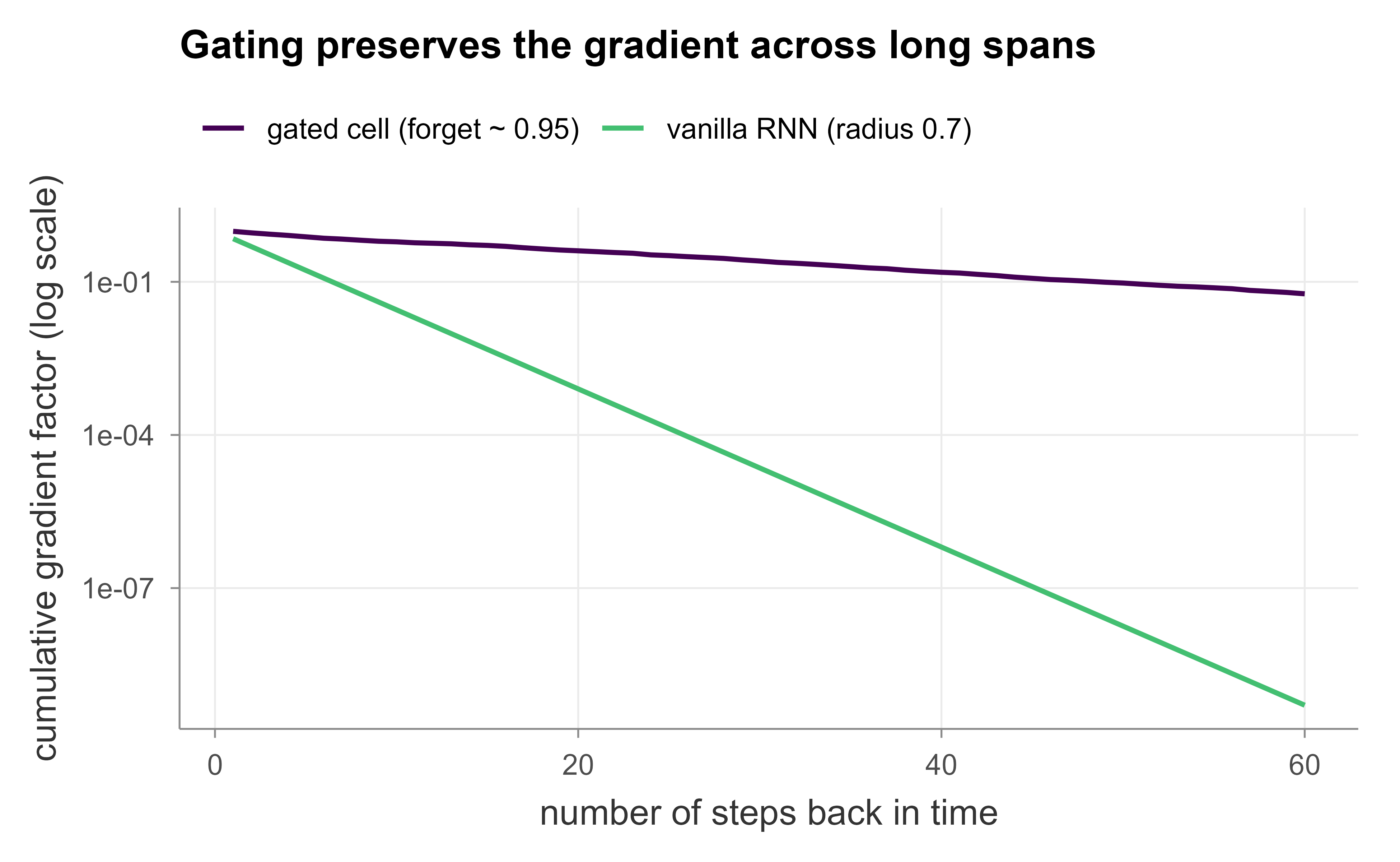
The gated curve stays within an order of magnitude of one across all sixty steps, while the vanilla curve has long since vanished. A learnable per-step coefficient, tuned toward one when long memory is needed, is the entire mechanism behind LSTMs and GRUs.
37.6.1 Training a real model
Fitting an LSTM or GRU on real data uses a deep learning backend. The following sketch with keras trains a small LSTM for sequence classification; it is shown but not run, since it requires a TensorFlow installation.
Show code
library(keras)

# x_train: integer-encoded sequences padded to length `maxlen`
# y_train: binary labels
model <- keras_model_sequential() |>
  layer_embedding(input_dim = vocab_size, output_dim = 32,
                  input_length = maxlen) |>
  layer_lstm(units = 64, dropout = 0.2, recurrent_dropout = 0.2) |>
  layer_dense(units = 1, activation = "sigmoid")

model |> compile(
  optimizer = "adam",
  loss      = "binary_crossentropy",
  metrics   = "accuracy"
)

# Gradient clipping (eq-rnn-clip) guards against exploding gradients;
# in keras pass clipnorm to the optimizer, e.g. optimizer_adam(clipnorm = 1.0).
history <- model |> fit(
  x_train, y_train,
  epochs = 10, batch_size = 64,
  validation_split = 0.2
)
The torch package offers an equivalent path with nn_lstm() or nn_gru() and a manual training loop, which exposes the gradient clipping step explicitly via nn_utils_clip_grad_norm_(). Either backend handles the BPTT bookkeeping automatically; the concepts that matter for getting it to train, the forget-gate bias initialization, gradient clipping, and choosing a sequence length that the gating can actually bridge, are all direct consequences of the analysis in this chapter.
37.7 Connections and Further Reading
RNNs sit at the intersection of several threads in this book. As neural sequence models they extend the feedforward networks of Chapter 15 with weight sharing across time. Their probabilistic reading as autoregressive models of a sequence links them to Chapter 77. The attention mechanism that fixed the encoder-decoder bottleneck grew into the Transformers of Chapter 38, which now dominate the tasks RNNs once owned. And the practice of learning compressed representations of inputs, central to the encoder half of a sequence-to-sequence model, connects to the representation learning ideas in Chapter 41.
Takeaways
The recurrence \(h_t = f(h_{t-1}, x_t)\) gives a neural model memory, but BPTT turns that memory into a product of Jacobians whose norm scales like \(\gamma^{t-k}\), so gradients vanish when \(\gamma < 1\) and explode when \(\gamma > 1\). Clipping tames the explosion; gating cures the vanishing by replacing the uncontrolled weight product with a learned, near-identity additive path. LSTMs and GRUs implement that path with forget and update gates. For long-range, large-scale sequence modelling, prefer Transformers; for streaming, small data, or tight resource budgets, a GRU or LSTM is still a strong choice.