Imagine you are trying to predict house prices and your first simple model is wrong in a patterned way: it overshoots cheap houses and undershoots expensive ones. A natural fix is to fit a second model to those leftover errors, add it to the first, look at what is still wrong, fit a third model to that, and keep going. Each new model is a small correction aimed at the part of the problem the running total has not yet captured. That, in one sentence, is gradient boosting: build a strong predictor by stacking many weak ones, where each weak learner is trained on the mistakes of the ensemble so far.
This idea turns out to be one of the most reliable workhorses in all of machine learning. On the kind of tabular data that fills spreadsheets and databases (rows of mixed numeric and categorical columns), gradient-boosted trees routinely win against neural networks and almost everything else. They are the default first thing many practitioners reach for.
The boosting chapter (Chapter 11) introduced the foundations: forward stagewise additive modeling, AdaBoost, and the basic gradient boosting machine. This chapter picks up where that left off and focuses on the modern gradient-boosted-tree systems that dominate tabular prediction in practice: XGBoost, LightGBM, and CatBoost. By the end you will be able to read these systems in two complementary ways. First, as an optimization story: each one performs functional gradient descent against a regularized objective, and the formulas they use for leaf values and splits fall directly out of that view. Second, as a set of practical knobs you actually turn, with runnable training and validation loss curves that show overfitting happening and early stopping catching it.
Note
This chapter assumes you have seen the boosting chapter (Chapter 11). If the phrase “fit a tree to the residuals” is not yet familiar, read that chapter first; here we move quickly from intuition to the regularized objective that the production systems optimize.
12.1 Boosting as Functional Gradient Descent
The opening picture (fit each new model to the leftover errors) is intuitive, but to design and tune real systems we need a precise version of it. The precise version reframes boosting as gradient descent, not over a few numbers in a parameter vector, but over the predictions themselves. This section builds that reframing one step at a time.
A boosted model is an additive expansion of base learners,
\[
F_M(x) = \sum_{m=1}^M \nu \, f_m(x),
\]
where each \(f_m\) is a small regression tree and \(\nu \in (0,1]\) is the learning rate. We build this expansion one term at a time. Given the current model \(F_{m-1}\), we add a new base learner \(f_m\) chosen to reduce the total loss
This is forward stagewise additive modeling: previously added terms stay fixed, and we only solve for the next one.1
Key idea
Treat the predictions \(F(x_1), \dots, F(x_n)\) as the quantities we are optimizing, one per training point. The loss \(\mathcal{L}\) is then an ordinary function of those \(n\) numbers, and we can do gradient descent on it just as we would on any other parameters.
Steepest descent on \(\mathcal{L}\) in this function space moves each prediction in the direction of the negative gradient. Define the pseudo-residual2 at observation \(i\) and step \(m\) as
We then fit the base learner \(f_m\) to the pseudo-residuals \(\{(x_i, r_{im})\}\) by least squares. Here is why a tree is the right tool: pure gradient descent would tell us how to nudge each of the \(n\) predictions individually, but that gives us no rule for predicting at a new \(x\) we have never seen. Fitting a tree to \(r_{im}\) forces the descent direction to be a function of \(x\), so it generalizes. The new tree points the whole model downhill in loss while still being something we can evaluate anywhere. After fitting, the leaf values can be re-optimized for the actual loss (a line search per leaf), and the tree is added with shrinkage \(\nu\).
Intuition
Gradient descent says “move in this direction.” A tree is how we make “this direction” into a reusable function of the features instead of a one-off adjustment to the training points.
12.1.1 The generic algorithm and the line search
It is worth writing the procedure once in full generality, because every system in this chapter is a special case of it. This is Friedman’s (2001) gradient boosting machine. We work in the function space \(\mathcal{H}\) of base learners (here, regression trees with \(J\) terminal nodes), and we seek \(F\) minimizing the empirical risk \(\mathcal{L}(F) = \sum_{i=1}^n l(y_i, F(x_i))\).
Initialize with the best constant, \(F_0 = \arg\min_{c} \sum_{i=1}^n l(y_i, c)\). For squared error this is \(\bar y\); for logistic loss it is the log-odds \(\log\frac{\bar y}{1-\bar y}\).
Fit a regression tree to \(\{(x_i, r_{im})\}\), giving terminal regions \(R_{jm}\), \(j = 1, \dots, J_m\).
For each region solve the one-dimensional line search \[
\gamma_{jm} = \arg\min_{\gamma} \sum_{x_i \in R_{jm}} l\big(y_i,\, F_{m-1}(x_i) + \gamma\big).
\tag{12.1}\]
Two subtleties deserve emphasis. First, the tree in step (b) is fit to the gradient by least squares regardless of the loss\(l\): the squared-error fit is what projects the unconstrained negative-gradient direction onto the space of trees, exactly as steepest descent projects the gradient onto a feasible direction. Second, the leaf values are then re-optimized in step (c) for the true loss \(l\), not the squared-error surrogate. For squared error the two coincide (the line search returns the leaf mean), which is why the simpler “fit to residuals” story is exact there. For other losses they differ, and skipping (c) costs accuracy. For logistic loss Equation 12.1 has no closed form, so Friedman uses a single Newton step per leaf, \[
\gamma_{jm} = \frac{\sum_{x_i \in R_{jm}} r_{im}}{\sum_{x_i \in R_{jm}} p_{i,m-1}(1 - p_{i,m-1})},
\] which is precisely the XGBoost leaf weight (with \(\lambda = 0\)) derived later. Friedman’s “MART” and XGBoost differ mainly in that XGBoost uses the Newton step to choose the tree structure too, not just the leaf values.
12.1.2 Why fit the gradient by least squares
The projection claim above can be made precise. In ideal (unconstrained) functional steepest descent we would move \(F\) by \(-\nabla \mathcal{L}\), i.e. set the increment at each training point equal to \(r_{im}\). We cannot realize an arbitrary vector \((r_{1m}, \dots, r_{nm})\) as a tree, so we pick the tree \(h\) most parallel to the negative gradient. Maximizing the cosine between the increment vector \((h(x_1), \dots, h(x_n))\) and the gradient, at fixed norm, is equivalent to \[
f_m = \arg\min_{h \in \mathcal{H}} \sum_{i=1}^n \big(r_{im} - h(x_i)\big)^2,
\] which is exactly the least-squares fit in step (b). The negative gradient is thus the target a tree should approximate as closely as possible, and squared error is the natural metric for “closely” because it measures Euclidean distance in the same prediction space the gradient lives in.
12.1.3 Squared error gives ordinary residuals
For squared error loss \(l(y, F) = \tfrac12 (y - F)^2\), the gradient with respect to \(F\) is
The pseudo-residual is exactly the ordinary residual, which recovers the “fit a tree to the residuals” algorithm from the boosting chapter (Chapter 11). The optimal leaf value for a terminal region is the mean of the residuals in that region. So the intuitive picture from the start of the chapter is not an analogy; for squared error it is literally what the gradient view prescribes.
12.1.3.1 L2 boosting as an operator and its shrinkage interpretation
For squared error the whole expansion has a clean linear-algebra form that exposes what boosting does to the bias-variance trade-off. Let each base learner be a fixed linear smoother, \(\hat r = S r\), where \(S \in \mathbb{R}^{n \times n}\) is the smoother (hat) matrix mapping a response vector to its fitted values (for a tree, \(S\) is the block-constant averaging operator induced by the terminal regions). Starting from \(F_0 = 0\) and using learning rate \(\nu\), the residual after \(m\) rounds is \(r^{(m)} = (I - \nu S) r^{(m-1)}\), so \[
r^{(m)} = (I - \nu S)^m\, y, \qquad \hat y^{(m)} = \big[I - (I - \nu S)^m\big]\, y.
\tag{12.2}\] The effective fit operator is \(B_m = I - (I - \nu S)^m\). If \(S\) has eigendecomposition with eigenvalues \(s_k \in [0,1]\) (true for symmetric averaging smoothers), then \(B_m\) has eigenvalues \[
b_k^{(m)} = 1 - (1 - \nu s_k)^m \;\xrightarrow{m \to \infty}\; 1 \quad (\text{for } s_k > 0).
\] The structure is illuminating. Components with large \(s_k\) (smooth, high-signal directions) are recovered after only a few rounds, while components with small \(s_k\) (rough, noise-like directions) are damped as \((1 - \nu s_k)^m\) and only enter slowly. Boosting is thus a regularization path: the number of rounds \(M\) plays the role of an inverse penalty, fitting structured signal first and noise last, which is exactly why early stopping works and why it behaves like ridge-type shrinkage in eigen-space (Bühlmann and Yu 2003). The degrees of freedom \(\operatorname{tr}(B_m)\) grow monotonically with \(m\), formalizing “more rounds means more flexibility.”
Note
Equation 12.2 also explains the learning-rate-versus-rounds duality quantitatively. For small \(\nu\), \(1 - (1-\nu s_k)^m \approx 1 - e^{-\nu s_k m}\), which depends on \(\nu\) and \(m\) only through the product \(\nu m\). Halving \(\nu\) and doubling \(m\) leaves the fit (to first order) unchanged, the precise statement behind the “two ends of the same lever” intuition.
The operator identity Equation 12.2 is exact, so we can confirm it in a line of base R: boost a fixed smoother by hand and check the residuals match \((I - \nu S)^m y\).
Show code
mat_pow<-function(M, p){R<-diag(nrow(M)); for(iinseq_len(p))R<-R%*%M; R}set.seed(1)n<-40S<-matrix(rnorm(n*n), n, n); S<-(S+t(S))/2# symmetric smootherS<-S/(max(abs(eigen(S, only.values =TRUE)$values))*2)# keep |eig| smally<-rnorm(n)nu<-0.3; m<-25# explicit stagewise boosting of the smoother SF<-rep(0, n)for(kinseq_len(m))F<-F+nu*as.vector(S%*%(y-F))# closed form from eq-l2opF_closed<-as.vector((diag(n)-mat_pow(diag(n)-nu*S, m))%*%y)max(abs(F-F_closed))# ~ machine epsilon#> [1] 3.197442e-14
12.1.4 Logistic loss gives probability residuals
The same machinery handles classification once we pick the right loss. The only change is the formula for the gradient; everything else (fit a tree to it, re-optimize leaves, shrink, repeat) is identical.
For binary classification with \(y_i \in \{0,1\}\), let \(F(x)\) be the log-odds (a real number) and \(p = \sigma(F) = 1/(1 + e^{-F})\).3 The logistic (binomial deviance) loss is
\[
l(y, F) = -\big[\, y \log p + (1-y) \log(1-p) \,\big] = \log\!\big(1 + e^{F}\big) - y F.
\]
Differentiating with respect to \(F\) and using \(\sigma'(F) = \sigma(F)(1-\sigma(F))\),
\[
\frac{\partial l}{\partial F} = \sigma(F) - y = p - y, \qquad r_{im} = y_i - p_{i,m-1}.
\]
The pseudo-residual is the difference between the observed label and the current predicted probability, a satisfying mirror of the regression case where it was observed minus predicted value. The second derivative (Hessian), which the next section uses to take a smarter step than plain gradient descent, is
\[
\frac{\partial^2 l}{\partial F^2} = p (1 - p).
\]
Note
The Hessian \(p(1-p)\) is largest when \(p \approx 0.5\) (the model is most uncertain) and shrinks toward zero as predictions become confident. XGBoost uses exactly this curvature to decide how big a step each leaf should take, which is the subject of the next section.
12.2 The Tuning Knobs and Their Roles
Before the production-system formulas, it helps to know what you will actually be turning. Every gradient-boosting library exposes essentially the same handful of parameters, and they all do one job: control where the model sits on the bias-variance spectrum. Too little flexibility and the model underfits; too much and it memorizes the training set. The knobs below are the levers for that trade-off.
Learning rate (shrinkage) \(\nu\): scales each tree’s contribution. Smaller \(\nu\) slows learning, which usually improves generalization but requires more trees. Think of it as taking many small, careful steps instead of a few large, greedy ones. \(\nu\) and the number of trees trade off against each other directly.
Number of trees (rounds) \(M\): more rounds keep reducing training loss, but validation loss eventually rises. This is the main overfitting control, and it is what early stopping monitors.
Tree depth / interaction order: a tree of depth \(d\) can model interactions among up to \(d\) features. Depth 1 (stumps) gives a purely additive model; deeper trees capture higher-order interactions at the cost of variance.
Subsampling rows (stochastic gradient boosting): fitting each tree on a random fraction of the rows decorrelates the trees and acts as a regularizer, often improving accuracy and speed.
Subsampling columns: sampling a fraction of features per tree or per split further decorrelates trees, in the same spirit as random forests (Chapter 13).
Intuition
The learning rate and the number of trees are two ends of the same lever. Halve the learning rate and you will roughly need to double the trees to fit the same amount. This is why we almost never tune them independently: we fix a small learning rate and let early stopping pick the count.
The pattern that holds across most tabular problems is worth memorizing: a small learning rate, moderate depth (often 3 to 8), some row and column subsampling, and the number of trees chosen by early stopping on a validation set. The rest of this chapter explains why these defaults work and shows them in code.
12.3 XGBoost: a Regularized, Second-Order Objective
So far we have used only the first derivative of the loss (the gradient). XGBoost (Chen and Guestrin 2016) makes two changes that account for much of its success. First, it writes down an explicit penalty for tree complexity and optimizes loss plus penalty together, rather than relying only on tree depth to control overfitting. Second, it uses the second derivative (the Hessian) as well as the first, which lets it take a Newton step instead of a plain gradient step and gives a clean, closed-form rule for both leaf values and split decisions. The payoff is that the algorithm’s core formulas are not heuristics; they are the exact solution to a well-defined optimization problem.
XGBoost optimizes a penalized objective that adds a complexity term for each tree \(f_k\),
where \(T\) is the number of leaves, \(w \in \mathbb{R}^T\) is the vector of leaf weights, \(\gamma\) penalizes adding leaves, and \(\lambda\) is an L2 penalty on the leaf weights. Read \(\Omega\) as a price list: every leaf you add costs \(\gamma\), and large leaf values are taxed by \(\lambda\). Splitting only pays off when it buys enough loss reduction to cover that price.
12.3.1 Newton step on the objective
We now derive the rules XGBoost uses. The strategy is to approximate the loss around the current prediction by a quadratic, because a quadratic is easy to minimize exactly. This is the same move Newton’s method makes in ordinary optimization, applied here per training point.
At boosting round \(t\) we add a tree \(f_t\), so the prediction becomes \(\hat y_i^{(t)} = \hat y_i^{(t-1)} + f_t(x_i)\). Take a second-order Taylor expansion of the loss around the current prediction, using the gradient and Hessian
A tree assigns every \(x_i\) to exactly one leaf. Let \(I_j = \{ i : x_i \text{ falls in leaf } j \}\) be the set of observations in leaf \(j\), where \(f_t(x_i) = w_j\). Group the sum by leaf,
Grouping by leaf is the step that makes everything tractable: because every point in a leaf gets the same weight \(w_j\), the whole objective splits into one independent little problem per leaf. We solve those next.
12.3.2 Optimal leaf weight and the structure score
For a fixed tree structure, each leaf weight is decoupled and the objective is quadratic in \(w_j\). Let \(G_j = \sum_{i \in I_j} g_i\) and \(H_j = \sum_{i \in I_j} h_i\). Setting the derivative to zero,
Lower is better, so \(\sum_j G_j^2 / (H_j + \lambda)\) measures how good a tree structure is.
Key idea
The structure score turns “how good is this tree shape?” into a single number we can compute without ever fitting the leaf values by trial and error. Every decision XGBoost makes about growing the tree reduces to comparing this score before and after a candidate change.
12.3.3 Split gain
The structure score evaluates a finished tree, but we build trees greedily, one split at a time. So we need the change in the score from a single split, which is the quantity the algorithm maximizes when choosing where to cut.
We grow the tree greedily. Consider splitting one leaf into a left child \(L\) and a right child \(R\). The reduction in the objective from making the split is the gain
The first two terms are the structure scores of the children, the third is the score of the parent before splitting, and \(\gamma\) is the cost of adding a leaf. A split is only kept when its gain is positive, which is a built-in form of pruning: the \(\gamma\) term and the \(\lambda\) shrinkage in the denominators both discourage splits that rely on few observations.4
It is worth seeing that this general machinery collapses to the familiar cases. For squared error, \(g_i = \hat y_i - y_i\) and \(h_i = 1\), so \(w_j^* = -G_j / (|I_j| + \lambda)\), a shrunken mean of the residuals: the residual-averaging rule from before, now with a regularization term in the denominator. For logistic loss, \(g_i = p_i - y_i\) and \(h_i = p_i(1-p_i)\), which is exactly the gradient and Hessian we derived in the classification subsection. The same two-line objective handles regression and classification by plugging in a different \(g\) and \(h\).
12.3.4 What min_child_weight and lambda actually do
Two regularizers in the structure score have a precise reading worth spelling out, because they are among the most useful knobs in practice. The denominator \(H_j + \lambda\) is the total Hessian mass in a leaf plus the L2 penalty. The quantity \(H_j = \sum_{i \in I_j} h_i\) is exactly what XGBoost calls the cover of a leaf, and the hyperparameter min_child_weight is a floor on it: a split is rejected if either child has \(H < \text{min\_child\_weight}\). For squared error \(h_i = 1\), so cover is just the number of points and min_child_weight is a minimum leaf size. For logistic loss \(h_i = p_i(1-p_i)\), so a leaf full of confidently classified points (each \(p_i(1-p_i) \approx 0\)) has tiny cover even if it contains many rows; min_child_weight then refuses to keep splitting regions the model already explains, a loss-aware version of “minimum samples per leaf.”
The role of \(\lambda\) is equally concrete. The optimal leaf weight \(w_j^* = -G_j/(H_j + \lambda)\) is the unregularized Newton step \(-G_j/H_j\) multiplied by the shrinkage factor \(H_j/(H_j + \lambda)\). Leaves with little curvature mass (few or low-confidence points) are shrunk hardest toward zero, which is exactly the behavior we want: trust the leaves backed by data, distrust the rest. Setting \(\lambda = 0\) and \(\gamma = 0\) recovers Friedman’s Newton-step MART; positive \(\lambda\) and \(\gamma\) are what make the structure score, and therefore split selection itself, regularization-aware.
12.3.5 Computational complexity
The cost of one boosting round is dominated by split finding. With \(n\) rows, \(d\) features, and a tree of depth \(D\), the exact greedy search of XGBoost pre-sorts each feature once (\(O(n d \log n)\) amortized via cached sorted blocks) and then, at each of the \(O(D)\) levels, scans every feature over every candidate threshold, accumulating \(G\) and \(H\) in a single linear pass. This gives \(O(d \cdot n \cdot D)\) per tree after sorting, or \(O(M \cdot d \cdot n \cdot D)\) for the full ensemble. The histogram method (LightGBM, and XGBoost’s hist) replaces the per-threshold scan with accumulation into \(b\) bins, costing \(O(d \cdot n)\) to build histograms per level (independent of the number of distinct values) plus \(O(d \cdot b)\) to scan them, with \(b \ll n\). A further trick is that a node’s histogram can be obtained by subtracting a sibling’s histogram from the parent’s, halving the build cost. Memory is \(O(n d)\) for the binned matrix, which is why histogram methods, not the exact method, are used at scale.
12.4 LightGBM, CatBoost, and the Speed Tricks
The objective and split formulas above describe what XGBoost computes. The remaining differences between the major libraries are mostly about how fast they compute it on large data, and how gracefully they handle categorical features. Understanding these tricks helps you choose a library and read its parameter list, even though the underlying boosting story is the same.
XGBoost’s original exact greedy split search scans every candidate split point on every feature, which is accurate but slow when there are many rows. LightGBM (Ke et al. 2017) trades a little precision for large speedups using four ideas:
Histogram-based splits: continuous features are bucketed into a fixed number of bins (for example 255). Split candidates are evaluated on the histogram of binned values rather than on raw sorted values, so split finding cost scales with the number of bins, not the number of distinct values. The per-row gradient and Hessian sums are accumulated per bin.5
Leaf-wise (best-first) growth: instead of growing all nodes at a given depth (level-wise), LightGBM repeatedly splits the leaf with the largest gain. This reaches lower loss for a given number of leaves but can overfit, so the number of leaves and a maximum depth are the main controls.
Gradient-based One-Side Sampling (GOSS): observations with large gradients are far from being fit well, so GOSS keeps all large-gradient rows and randomly subsamples the small-gradient rows, reweighting the kept small-gradient rows to keep the gradient sums roughly unbiased. This shrinks the training set while preserving the important signal.
Exclusive Feature Bundling (EFB): in sparse data many features are rarely nonzero at the same time. EFB bundles such mutually exclusive features into a single feature, reducing the effective feature count with little information loss.
Warning
LightGBM’s leaf-wise growth is powerful but easy to overfit with. A tree controlled only by num_leaves can grow much deeper along one branch than a level-wise tree of the same leaf count. If you see training loss far below validation loss, cap max_depth or lower num_leaves before touching anything else.
CatBoost rounds out the trio with a different concern: bias. Ordinary gradient boosting uses the same rows to both fit the model and compute the residuals it will fit next, which subtly leaks information and biases the predictions, an effect its authors call prediction shift. CatBoost addresses this with ordered boosting, which computes the residual for each observation using a model trained only on earlier observations in a random permutation. It also has strong native handling of categorical features through ordered target statistics, so categorical columns can be passed in directly rather than one-hot encoded by hand.
12.4.0.1 Prediction shift made precise
The bias has a clean source. At round \(t\) the gradient \(g_i = \partial l(y_i, F_{t-1}(x_i))/\partial F_{t-1}(x_i)\) is evaluated at \(F_{t-1}\), which was itself fit using \((x_i, y_i)\). The conditional distribution of \(g_i \mid x_i\) over the training set therefore differs from the distribution at a fresh test point \(x\), because for the training point the model has already partly absorbed \(y_i\). The fitted increment \(f_t\) is an estimate of \(\mathbb{E}[g \mid x]\), but it is trained on targets whose conditional law is shifted; the resulting \(f_t(x)\) is a biased estimate of the population gradient, and the bias compounds over rounds. Prokhorenkova et al. (2018) show this bias is \(O(1/n)\) in magnitude but does not vanish in the relevant finite-sample regimes. Ordered boosting removes it by maintaining, for a random permutation \(\sigma\), a model \(M_i\) for each \(i\) that is trained only on the points preceding \(i\) in \(\sigma\); the residual for \(i\) is then computed with \(M_i\), which has never seen \(y_i\). This is an online, leakage-free estimate of the gradient at the cost of maintaining several supporting models.
12.4.0.2 Ordered target statistics
The same leakage problem afflicts the simplest categorical encoding, target (mean) encoding, which replaces a category \(c\) by the average response of rows with that category. Computed on all rows, \(\hat\mu_c = \frac{1}{|\{i: x_i = c\}|}\sum_{i: x_i=c} y_i\) uses \(y_i\) to encode row \(i\), leaking the target directly. CatBoost’s ordered target statistic fixes this by, again, using only the prefix of a random permutation: \[
\hat{x}_i = \frac{\sum_{j < i,\; x_j = x_i} y_j + a\, p}{\sum_{j < i,\; x_j = x_i} 1 + a},
\] where \(p\) is a prior (the global mean) and \(a > 0\) is a smoothing strength. The numerator and denominator use only earlier rows, so \(y_i\) never enters its own encoding; the prior term \(a p\) is a Bayesian shrinkage that stabilizes rare categories, exactly the same regularization motive as \(\lambda\) in the leaf weight. This turns a high-cardinality categorical into a single informative numeric feature without one-hot blowup and without leakage.
When to use this
Reach for LightGBM when you have many rows and want speed; reach for CatBoost when categorical features dominate and you want sensible defaults with minimal preprocessing; reach for XGBoost as a mature, widely supported baseline. In practice all three are competitive, and the choice often comes down to ecosystem and familiarity.
12.5 Theoretical Properties and Connections
Beyond the mechanics, gradient boosting sits inside a well-understood statistical picture. Three results frame what it can and cannot do.
Boosting as coordinate descent in a basis. Consider the dictionary of all possible trees \(\{h_1, h_2, \dots\}\) and the linear model \(F = \sum_k \beta_k h_k\). Forward stagewise boosting with infinitesimal steps (\(\nu \to 0\)) traces out, under mild conditions, the same path as the L1-regularized (lasso) solution \(\min_\beta \sum_i l(y_i, \sum_k \beta_k h_k(x_i)) + t\lVert\beta\rVert_1\) as the budget \(t\) grows (Efron et al. 2004; Rosset, Zhu and Hastie 2004). This is the precise sense in which shrinkage plus many rounds gives an implicit L1 penalty over base learners: small \(\nu\) does not merely slow learning, it changes which solution you converge toward, favoring sparse combinations of trees. It also explains why very small \(\nu\) with early stopping reliably outperforms large \(\nu\): large steps overshoot the regularization path.
Consistency. For appropriate losses and base-learner classes, boosting with early stopping is consistent: the population risk of \(F_M\) converges to the Bayes risk as \(n \to \infty\), provided \(M = M_n\) grows at a controlled rate and the step size is small (Zhang and Yu 2005; Bühlmann 2006). The key tension is that \(\mathcal{L}(F_M) \to 0\) on the training set as \(M \to \infty\) (interpolation), so \(M\) must be stopped before overfitting; consistency results give rates for how fast \(M_n\) may grow. Without early stopping or shrinkage, boosting to convergence can overfit, especially with noisy labels, which is the theoretical counterpart to the upturn in Figure 12.1.
Bias-variance and tree depth. The interaction order is set by depth: a depth-\(D\) tree is a sum of basis functions each involving at most \(D\) features, so the ensemble is a member of the ANOVA-style functional class with interactions up to order \(D\) (the connection to generalized additive models in Chapter 6 is exact at \(D=1\), where boosting fits an additive model). Increasing \(D\) lowers approximation bias but raises variance and the chance of fitting spurious high-order interactions. Friedman’s recommendation of \(4 \le J \le 8\) leaves (\(D \approx 2\) to \(3\)) reflects that most real interaction structure is low-order.
Failure modes
Gradient boosting breaks in characteristic ways. (1) It does not extrapolate: trees are piecewise constant, so predictions are flat outside the training range, unlike linear models. (2) It is sensitive to label noise; because it chases residuals, mislabeled points get fit with ever-deeper trees, and a heavy-tailed loss such as squared error lets a few outliers dominate (use Huber or quantile loss instead). (3) Severe class imbalance makes the Hessian \(p(1-p)\) tiny for the majority class, starving minority-class splits of cover; reweighting or scale_pos_weight is needed. (4) With \(M\) too large and no validation set it will silently interpolate the training data.
12.6 Simulation: Loss Curves, Learning Rates, and Importance
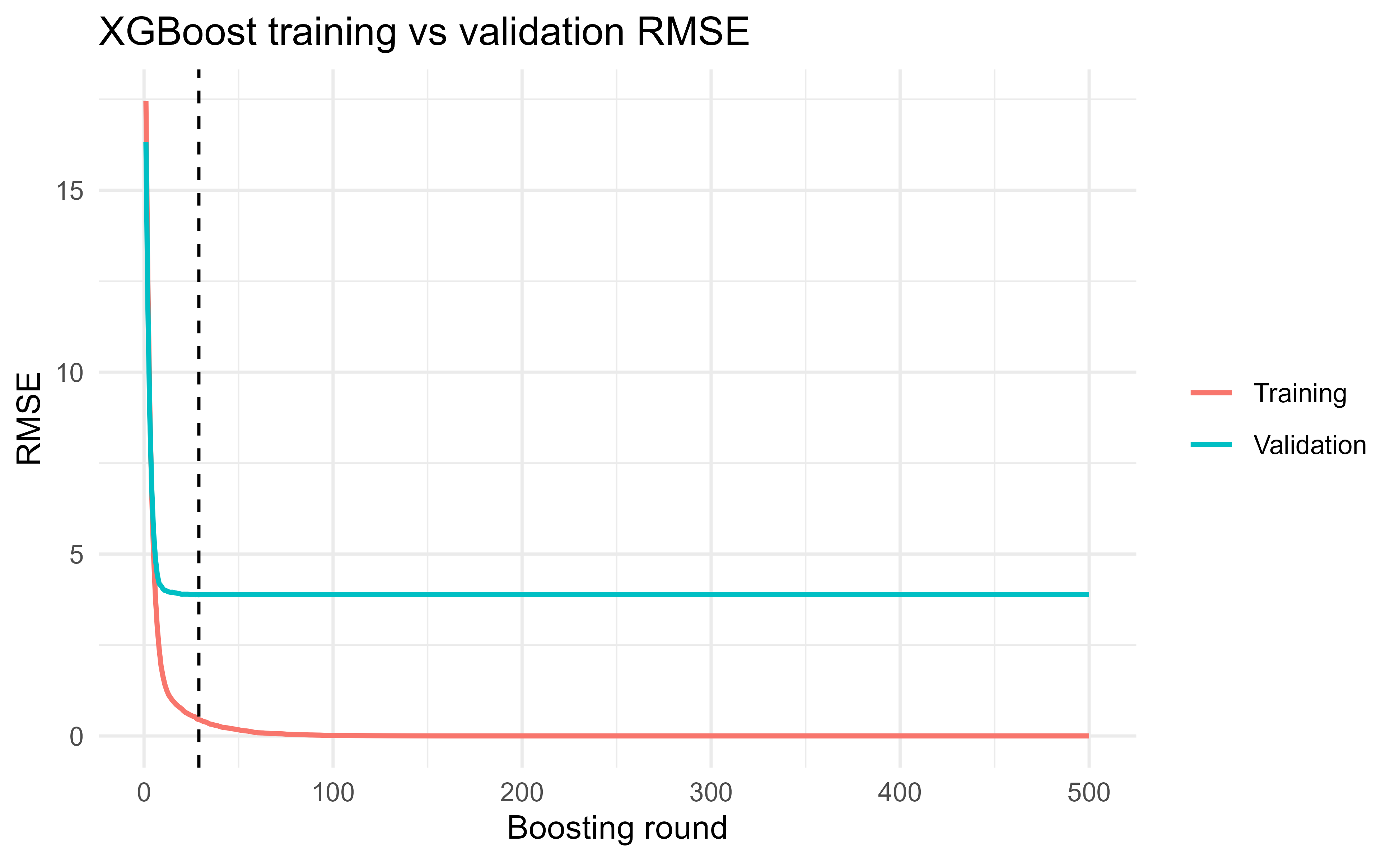
Theory predicts that training loss falls forever while validation loss eventually turns around; this section makes that prediction visible. We use the Boston housing data from ISLR2 as a regression example, where the goal is to predict the median home value medv from neighborhood characteristics. We hold out a validation set, train XGBoost while recording training and validation RMSE at every round, and plot the curves to see overfitting happen and to locate where early stopping would cut off. We then compare learning rates and read off feature importance.
The setup splits the data 70/30 and wraps each part in an xgb.DMatrix, XGBoost’s internal data structure:
We train a deliberately under-regularized model (large learning rate, moderate depth, many rounds, no subsampling) so the validation curve turns upward and the overfitting is plain to see. The watchlist tells XGBoost to evaluate RMSE on both sets after every round and store the history in evaluation_log.
best_round<-which.min(log_df$valid_rmse)ggplot(log_df, aes(x =iter))+geom_line(aes(y =train_rmse, color ="Training"))+geom_line(aes(y =valid_rmse, color ="Validation"))+geom_vline(xintercept =best_round, linetype ="dashed")+labs(x ="Boosting round", y ="RMSE", color =NULL, title ="XGBoost training vs validation RMSE")+theme_minimal()best_round#> [1] 29min(log_df$valid_rmse)#> [1] 3.87984
Figure 12.1: Training and validation RMSE versus number of boosting rounds. Training error keeps falling while validation error flattens then rises, the signature of overfitting. The dashed line marks the round with minimum validation RMSE (the early-stopping point).
Figure 12.1 is the whole lesson in one picture. The training curve marches steadily downward, because adding trees can always fit the training data a little better. The validation curve drops at first, because early trees capture real structure, but then bottoms out and creeps back up, because later trees start fitting noise that does not generalize. The dashed line marks the round where validation RMSE is lowest; everything to the right of it is overfitting we would rather avoid.
Tip
Reading a loss curve is the single most useful diagnostic in boosting. A validation curve that is still falling means you stopped too early (train longer or lower the learning rate). One that turned up long ago means you trained too long. A flat curve far above the training curve means the model is too flexible (reduce depth or add subsampling).
Eyeballing the dashed line is fine for a plot, but we do not want to retrain hundreds of rounds just to throw most away. Early stopping automates picking that round: training continues until the validation metric fails to improve for a fixed number of rounds (early_stopping_rounds), then stops and keeps the best iteration. Here we also switch to sensible regularization (smaller learning rate, shallower trees, row and column subsampling) so the model generalizes better.
The reported best_iteration is the round XGBoost will use for prediction, and best_score is the validation RMSE there. Note that this regularized model stops after far fewer effective rounds and reaches a similar or better error than the over-trained one above, with much less risk of overfitting.
12.6.1 Comparing learning rates
To see the learning-rate-versus-rounds trade-off concretely, we sweep a few learning rates, each with its own early stopping, and record how many rounds each one needs and the best validation RMSE it reaches. The expectation from theory is that smaller learning rates need more rounds but tend to reach a comparable or better minimum.
The best_round column confirms the pattern: as the learning rate shrinks, the number of rounds needed climbs sharply, while the validation RMSE stays in a narrow band. This is exactly why the standard recipe is to fix a small learning rate and let early stopping spend whatever rounds are required, rather than tuning the round count by hand.
12.6.2 Feature importance
A fitted booster also tells us which features mattered. XGBoost reports three importance measures: gain (the average split-gain contribution of a feature, summed over the splits that use it), cover (the average number of observations affected by its splits), and frequency (how often it is used). Gain is the usual ranking because it reflects how much each feature actually reduced the loss.
Show code
imp<-xgb.importance(model =fit_es)knitr::kable(imp, digits =4, caption ="XGBoost feature importance (gain, cover, frequency) for the Boston model.")
Table 12.1: XGBoost feature importance (gain, cover, frequency) for the Boston model.
Feature
Gain
Cover
Frequency
rm
0.5085
0.1697
0.1440
lstat
0.1742
0.1561
0.1268
nox
0.0809
0.0797
0.0960
ptratio
0.0686
0.0404
0.0431
dis
0.0454
0.1830
0.1329
crim
0.0413
0.1260
0.1895
age
0.0231
0.1193
0.1378
indus
0.0207
0.0355
0.0412
chas
0.0174
0.0104
0.0105
tax
0.0157
0.0538
0.0462
rad
0.0034
0.0146
0.0222
zn
0.0007
0.0114
0.0098
The ranking in Table 12.1 is intuitive for housing data: rm (average number of rooms) and lstat (percent lower-status population) dominate, which matches both economic intuition and the linear-model coefficients you would get on the same data.
Warning
Importance scores describe what the model used, not causal effect, and they can be unstable when features are correlated (the model may “credit” one of two redundant features almost arbitrarily). Treat them as a rough guide for the model at hand, not as a measure of how the world works. For more careful attribution, the interpretable machine learning chapter (Chapter 35) covers SHAP values and partial dependence.
12.6.3 LightGBM on the same data
To show that the workflow carries over, we fit LightGBM on the same train/validation split. The API differs in surface details (lgb.Dataset instead of xgb.DMatrix, feature_fraction/bagging_fraction instead of colsample_bytree/subsample), but the logic (early stopping on a validation set, then read importance) is identical. Its key controls are num_leaves, which governs the leaf-wise growth discussed above, and learning_rate.
Table 12.2: LightGBM feature importance for the Boston model.
Feature
Gain
Cover
Frequency
rm
0.6058
0.2221
0.1763
lstat
0.2734
0.2909
0.2059
crim
0.0338
0.0687
0.1113
nox
0.0284
0.0953
0.1020
dis
0.0259
0.0894
0.1187
ptratio
0.0128
0.0719
0.0742
age
0.0083
0.0630
0.0853
tax
0.0048
0.0413
0.0575
rad
0.0025
0.0312
0.0371
chas
0.0022
0.0126
0.0056
indus
0.0020
0.0122
0.0223
zn
0.0001
0.0014
0.0037
Reassuringly, the LightGBM ranking in Table 12.2 lands on the same top features (rm and lstat) and a similar validation error, despite its different growth strategy and split search. When two well-tuned boosting libraries agree on both the ranking and the error, that is a good sign the signal is real and not an artifact of one implementation.
12.7 Practical Notes
Everything above comes together into a short, repeatable workflow. The following order is what works in practice on most tabular problems:
Fix a small learning rate (0.05 or 0.1), set the number of rounds high, and let early stopping choose the actual count.
Tune tree shape next: max_depth or num_leaves, and the minimum child weight or minimum data per leaf.
Tune the subsampling fractions: subsample/bagging_fraction for rows and colsample_bytree/feature_fraction for columns.
Add L1/L2 penalties (alpha, lambda) and the split-cost gamma last, only if the model still overfits.
Optionally, after the shape is settled, drop the learning rate further and retrain with early stopping for a small accuracy gain at the cost of more rounds.
Warning
Early stopping needs a validation set (or cross-validation via xgb.cv and lgb.cv) and a metric to monitor, and that set has been used for model selection. Always report your final performance on a separate test set the model never saw during stopping, or you will report an optimistic number.
A recurring practical question is how each library handles categorical features and missing values, since this is where the most preprocessing time is spent. The three systems differ:
XGBoost takes a numeric matrix, so categoricals must be one-hot or target encoded beforehand. It handles missing values natively: at each split a default direction is learned, and missing values go that way, so you can pass NA without imputation.
LightGBM handles missing values natively and can treat integer-coded columns as categorical when told which columns they are (categorical_feature), using an optimized partition of categories rather than one-hot expansion.
CatBoost is built around categorical features and applies ordered target statistics internally, which avoids manual encoding and reduces leakage.
Tip
The native missing-value handling in these libraries is a real convenience, but it makes “missing” itself a signal the model can use. If your data is missing for reasons related to the target (informative missingness), that can help; if it is missing by accident, double-check that the learned default directions are not picking up a quirk of your collection process.
12.7.1 Monotonic and interaction constraints
All three libraries can enforce that the prediction is monotone in a feature (monotone_constraints), which is useful when domain knowledge demands it (price should not decrease in square footage). The mechanism follows directly from the split-gain machinery: when a split on a monotone-constrained feature is considered, the candidate is only kept if the resulting left and right leaf weights respect the required ordering, and downstream splits are bounded so the constraint cannot be violated lower in the tree. This is a hard constraint on the function class, not a penalty, so it can only reduce training fit, but it often improves generalization and always improves trust. Similarly, interaction_constraints restrict which features may appear together on a single root-to-leaf path, capping the interaction order between specified groups, which is the practical lever for the depth/interaction-order trade-off from Section 12.5.
Note
Because boosted trees cannot extrapolate (failure mode 1 above), monotone constraints are especially valuable at the edges of the training distribution: they let you guarantee sensible behavior in regions where the data is sparse and the unconstrained model would otherwise produce flat or erratic predictions.
To summarize the chapter: gradient boosting is functional gradient descent that builds an additive model of trees, each fit to the negative gradient of the loss. XGBoost sharpens this with a regularized, second-order objective whose leaf weights and split gains have closed forms. LightGBM and CatBoost keep that core and add speed and categorical-handling tricks. In practice you fix a small learning rate, let early stopping pick the number of trees, and tune tree shape and subsampling around that, watching the validation loss curve the entire time.
12.8 Further Reading
Friedman, J. H. (2001). Greedy function approximation: a gradient boosting machine. Annals of Statistics. The functional gradient descent view used throughout this chapter.
Chen, T. and Guestrin, C. (2016). XGBoost: A scalable tree boosting system. KDD. The regularized objective, second-order split gain, and systems design.
Ke, G. et al. (2017). LightGBM: A highly efficient gradient boosting decision tree. NeurIPS. Histogram splits, GOSS, and EFB.
Prokhorenkova, L. et al. (2018). CatBoost: unbiased boosting with categorical features. NeurIPS. Prediction shift, ordered boosting, and ordered target statistics.
Bühlmann, P. and Yu, B. (2003). Boosting with the L2 loss. JASA. The operator/eigenvalue view of L2 boosting and its shrinkage interpretation.
Rosset, S., Zhu, J. and Hastie, T. (2004). Boosting as a regularized path to a maximum margin classifier. JMLR. The implicit L1 (lasso) path of infinitesimal forward stagewise boosting.
Zhang, T. and Yu, B. (2005). Boosting with early stopping: convergence and consistency. Annals of Statistics. Consistency and stopping rates.
Refitting all the earlier terms at every step would be the “fully corrective” version. Keeping them frozen is cheaper and, with shrinkage, works better in practice because it limits how aggressively the model adapts to the training data.↩︎
Called a “pseudo”-residual because for a general loss it is not literally the observed-minus-predicted difference; it is the negative gradient of the loss, which only coincides with the ordinary residual for squared error, as we show next.↩︎
Working in log-odds space keeps \(F\) unconstrained on the whole real line, which is what lets us add trees freely. The sigmoid \(\sigma\) maps the running total back to a probability in \((0,1)\) only when we want to read off \(p\).↩︎
This is why \(\gamma\) is sometimes called min_split_loss: it is the minimum gain a split must earn to be worth keeping. Notice the family resemblance between split gain here and the impurity-reduction criterion of an ordinary CART tree (Chapter 8); XGBoost has simply replaced impurity with a loss-and-penalty-aware score.↩︎
XGBoost later added its own histogram method (tree_method = "hist"), so this is no longer unique to LightGBM. The other three tricks below are more distinctive.↩︎
Source Code
# Gradient Boosting in Practice {#sec-gradient-boosting}```{r}#| include: falsesource("_common.R")```Imagine you are trying to predict house prices and your first simple model is wrong in a patterned way: it overshoots cheap houses and undershoots expensive ones. A natural fix is to fit a second model to those leftover errors, add it to the first, look at what is still wrong, fit a third model to that, and keep going. Each new model is a small correction aimed at the part of the problem the running total has not yet captured. That, in one sentence, is gradient boosting: build a strong predictor by stacking many weak ones, where each weak learner is trained on the mistakes of the ensemble so far.This idea turns out to be one of the most reliable workhorses in all of machine learning. On the kind of tabular data that fills spreadsheets and databases (rows of mixed numeric and categorical columns), gradient-boosted trees routinely win against neural networks and almost everything else. They are the default first thing many practitioners reach for.The boosting chapter (@sec-boosting) introduced the foundations: forward stagewise additive modeling, AdaBoost, and the basic gradient boosting machine. This chapter picks up where that left off and focuses on the modern gradient-boosted-tree systems that dominate tabular prediction in practice: XGBoost, LightGBM, and CatBoost. By the end you will be able to read these systems in two complementary ways. First, as an optimization story: each one performs functional gradient descent against a regularized objective, and the formulas they use for leaf values and splits fall directly out of that view. Second, as a set of practical knobs you actually turn, with runnable training and validation loss curves that show overfitting happening and early stopping catching it.::: {.callout-note}This chapter assumes you have seen the boosting chapter (@sec-boosting). If the phrase "fit a tree to the residuals" is not yet familiar, read that chapter first; here we move quickly from intuition to the regularized objective that the production systems optimize.:::## Boosting as Functional Gradient DescentThe opening picture (fit each new model to the leftover errors) is intuitive, but to design and tune real systems we need a precise version of it. The precise version reframes boosting as gradient descent, not over a few numbers in a parameter vector, but over the predictions themselves. This section builds that reframing one step at a time.A boosted model is an additive expansion of base learners,$$F_M(x) = \sum_{m=1}^M \nu \, f_m(x),$$where each $f_m$ is a small regression tree and $\nu \in (0,1]$ is the learning rate. We build this expansion one term at a time. Given the current model $F_{m-1}$, we add a new base learner $f_m$ chosen to reduce the total loss$$\mathcal{L}(F) = \sum_{i=1}^n l\big(y_i, F(x_i)\big).$$This is forward stagewise additive modeling: previously added terms stay fixed, and we only solve for the next one.^[Refitting all the earlier terms at every step would be the "fully corrective" version. Keeping them frozen is cheaper and, with shrinkage, works better in practice because it limits how aggressively the model adapts to the training data.]::: {.callout-important title="Key idea"}Treat the predictions $F(x_1), \dots, F(x_n)$ as the quantities we are optimizing, one per training point. The loss $\mathcal{L}$ is then an ordinary function of those $n$ numbers, and we can do gradient descent on it just as we would on any other parameters.:::Steepest descent on $\mathcal{L}$ in this function space moves each prediction in the direction of the negative gradient. Define the pseudo-residual^[Called a "pseudo"-residual because for a general loss it is not literally the observed-minus-predicted difference; it is the negative gradient of the loss, which only coincides with the ordinary residual for squared error, as we show next.] at observation $i$ and step $m$ as$$r_{im} = - \left[ \frac{\partial l(y_i, F(x_i))}{\partial F(x_i)} \right]_{F = F_{m-1}}.$$We then fit the base learner $f_m$ to the pseudo-residuals $\{(x_i, r_{im})\}$ by least squares. Here is why a tree is the right tool: pure gradient descent would tell us how to nudge each of the $n$ predictions individually, but that gives us no rule for predicting at a new $x$ we have never seen. Fitting a tree to $r_{im}$ forces the descent direction to be a function of $x$, so it generalizes. The new tree points the whole model downhill in loss while still being something we can evaluate anywhere. After fitting, the leaf values can be re-optimized for the actual loss (a line search per leaf), and the tree is added with shrinkage $\nu$.::: {.callout-tip title="Intuition"}Gradient descent says "move in this direction." A tree is how we make "this direction" into a reusable function of the features instead of a one-off adjustment to the training points.:::### The generic algorithm and the line search {#sec-gradient-boosting-generic}It is worth writing the procedure once in full generality, because every system in this chapter is a special case of it. This is Friedman's (2001) gradient boosting machine. We work in the function space $\mathcal{H}$ of base learners (here, regression trees with $J$ terminal nodes), and we seek $F$ minimizing the empirical risk $\mathcal{L}(F) = \sum_{i=1}^n l(y_i, F(x_i))$.1. Initialize with the best constant, $F_0 = \arg\min_{c} \sum_{i=1}^n l(y_i, c)$. For squared error this is $\bar y$; for logistic loss it is the log-odds $\log\frac{\bar y}{1-\bar y}$.2. For $m = 1, \dots, M$: a. Compute pseudo-residuals $r_{im} = -\partial l(y_i, F(x_i)) / \partial F(x_i)\big|_{F_{m-1}}$. b. Fit a regression tree to $\{(x_i, r_{im})\}$, giving terminal regions $R_{jm}$, $j = 1, \dots, J_m$. c. For each region solve the one-dimensional line search $$ \gamma_{jm} = \arg\min_{\gamma} \sum_{x_i \in R_{jm}} l\big(y_i,\, F_{m-1}(x_i) + \gamma\big). $$ {#eq-gradient-boosting-linesearch} d. Update $F_m(x) = F_{m-1}(x) + \nu \sum_{j=1}^{J_m} \gamma_{jm}\, \mathbb{1}(x \in R_{jm})$.Two subtleties deserve emphasis. First, the tree in step (b) is fit to the gradient by **least squares regardless of the loss** $l$: the squared-error fit is what projects the unconstrained negative-gradient direction onto the space of trees, exactly as steepest descent projects the gradient onto a feasible direction. Second, the leaf values are then **re-optimized** in step (c) for the true loss $l$, not the squared-error surrogate. For squared error the two coincide (the line search returns the leaf mean), which is why the simpler "fit to residuals" story is exact there. For other losses they differ, and skipping (c) costs accuracy. For logistic loss @eq-gradient-boosting-linesearch has no closed form, so Friedman uses a single Newton step per leaf,$$\gamma_{jm} = \frac{\sum_{x_i \in R_{jm}} r_{im}}{\sum_{x_i \in R_{jm}} p_{i,m-1}(1 - p_{i,m-1})},$$which is precisely the XGBoost leaf weight (with $\lambda = 0$) derived later. Friedman's "MART" and XGBoost differ mainly in that XGBoost uses the Newton step to choose the tree **structure** too, not just the leaf values.### Why fit the gradient by least squaresThe projection claim above can be made precise. In ideal (unconstrained) functional steepest descent we would move $F$ by $-\nabla \mathcal{L}$, i.e. set the increment at each training point equal to $r_{im}$. We cannot realize an arbitrary vector $(r_{1m}, \dots, r_{nm})$ as a tree, so we pick the tree $h$ most parallel to the negative gradient. Maximizing the cosine between the increment vector $(h(x_1), \dots, h(x_n))$ and the gradient, at fixed norm, is equivalent to$$f_m = \arg\min_{h \in \mathcal{H}} \sum_{i=1}^n \big(r_{im} - h(x_i)\big)^2,$$which is exactly the least-squares fit in step (b). The negative gradient is thus the target a tree should approximate as closely as possible, and squared error is the natural metric for "closely" because it measures Euclidean distance in the same prediction space the gradient lives in.### Squared error gives ordinary residualsFor squared error loss $l(y, F) = \tfrac12 (y - F)^2$, the gradient with respect to $F$ is$$\frac{\partial l}{\partial F} = -(y - F), \qquad r_{im} = y_i - F_{m-1}(x_i).$$The pseudo-residual is exactly the ordinary residual, which recovers the "fit a tree to the residuals" algorithm from the boosting chapter (@sec-boosting). The optimal leaf value for a terminal region is the mean of the residuals in that region. So the intuitive picture from the start of the chapter is not an analogy; for squared error it is literally what the gradient view prescribes.#### L2 boosting as an operator and its shrinkage interpretation {#sec-gradient-boosting-l2}For squared error the whole expansion has a clean linear-algebra form that exposes what boosting does to the bias-variance trade-off. Let each base learner be a fixed linear smoother, $\hat r = S r$, where $S \in \mathbb{R}^{n \times n}$ is the smoother (hat) matrix mapping a response vector to its fitted values (for a tree, $S$ is the block-constant averaging operator induced by the terminal regions). Starting from $F_0 = 0$ and using learning rate $\nu$, the residual after $m$ rounds is $r^{(m)} = (I - \nu S) r^{(m-1)}$, so$$r^{(m)} = (I - \nu S)^m\, y, \qquad \hat y^{(m)} = \big[I - (I - \nu S)^m\big]\, y.$$ {#eq-gradient-boosting-l2op}The effective fit operator is $B_m = I - (I - \nu S)^m$. If $S$ has eigendecomposition with eigenvalues $s_k \in [0,1]$ (true for symmetric averaging smoothers), then $B_m$ has eigenvalues$$b_k^{(m)} = 1 - (1 - \nu s_k)^m \;\xrightarrow{m \to \infty}\; 1 \quad (\text{for } s_k > 0).$$The structure is illuminating. Components with large $s_k$ (smooth, high-signal directions) are recovered after only a few rounds, while components with small $s_k$ (rough, noise-like directions) are damped as $(1 - \nu s_k)^m$ and only enter slowly. Boosting is thus a **regularization path**: the number of rounds $M$ plays the role of an inverse penalty, fitting structured signal first and noise last, which is exactly why early stopping works and why it behaves like ridge-type shrinkage in eigen-space (Bühlmann and Yu 2003). The degrees of freedom $\operatorname{tr}(B_m)$ grow monotonically with $m$, formalizing "more rounds means more flexibility."::: {.callout-note}@eq-gradient-boosting-l2op also explains the learning-rate-versus-rounds duality quantitatively. For small $\nu$, $1 - (1-\nu s_k)^m \approx 1 - e^{-\nu s_k m}$, which depends on $\nu$ and $m$ only through the product $\nu m$. Halving $\nu$ and doubling $m$ leaves the fit (to first order) unchanged, the precise statement behind the "two ends of the same lever" intuition.:::The operator identity @eq-gradient-boosting-l2op is exact, so we can confirm it in a line of base R: boost a fixed smoother by hand and check the residuals match $(I - \nu S)^m y$.```{r gb-l2-verify}mat_pow <-function(M, p) { R <-diag(nrow(M)); for (i inseq_len(p)) R <- R %*% M; R }set.seed(1)n <-40S <-matrix(rnorm(n * n), n, n); S <- (S +t(S)) /2# symmetric smootherS <- S / (max(abs(eigen(S, only.values =TRUE)$values)) *2) # keep |eig| smally <-rnorm(n)nu <-0.3; m <-25# explicit stagewise boosting of the smoother SF <-rep(0, n)for (k inseq_len(m)) F <- F + nu *as.vector(S %*% (y - F))# closed form from eq-l2opF_closed <-as.vector((diag(n) -mat_pow(diag(n) - nu * S, m)) %*% y)max(abs(F - F_closed)) # ~ machine epsilon```### Logistic loss gives probability residualsThe same machinery handles classification once we pick the right loss. The only change is the formula for the gradient; everything else (fit a tree to it, re-optimize leaves, shrink, repeat) is identical.For binary classification with $y_i \in \{0,1\}$, let $F(x)$ be the log-odds (a real number) and $p = \sigma(F) = 1/(1 + e^{-F})$.^[Working in log-odds space keeps $F$ unconstrained on the whole real line, which is what lets us add trees freely. The sigmoid $\sigma$ maps the running total back to a probability in $(0,1)$ only when we want to read off $p$.] The logistic (binomial deviance) loss is$$l(y, F) = -\big[\, y \log p + (1-y) \log(1-p) \,\big] = \log\!\big(1 + e^{F}\big) - y F.$$Differentiating with respect to $F$ and using $\sigma'(F) = \sigma(F)(1-\sigma(F))$,$$\frac{\partial l}{\partial F} = \sigma(F) - y = p - y, \qquad r_{im} = y_i - p_{i,m-1}.$$The pseudo-residual is the difference between the observed label and the current predicted probability, a satisfying mirror of the regression case where it was observed minus predicted value. The second derivative (Hessian), which the next section uses to take a smarter step than plain gradient descent, is$$\frac{\partial^2 l}{\partial F^2} = p (1 - p).$$::: {.callout-note}The Hessian $p(1-p)$ is largest when $p \approx 0.5$ (the model is most uncertain) and shrinks toward zero as predictions become confident. XGBoost uses exactly this curvature to decide how big a step each leaf should take, which is the subject of the next section.:::## The Tuning Knobs and Their RolesBefore the production-system formulas, it helps to know what you will actually be turning. Every gradient-boosting library exposes essentially the same handful of parameters, and they all do one job: control where the model sits on the bias-variance spectrum. Too little flexibility and the model underfits; too much and it memorizes the training set. The knobs below are the levers for that trade-off.- Learning rate (shrinkage) $\nu$: scales each tree's contribution. Smaller $\nu$ slows learning, which usually improves generalization but requires more trees. Think of it as taking many small, careful steps instead of a few large, greedy ones. $\nu$ and the number of trees trade off against each other directly.- Number of trees (rounds) $M$: more rounds keep reducing training loss, but validation loss eventually rises. This is the main overfitting control, and it is what early stopping monitors.- Tree depth / interaction order: a tree of depth $d$ can model interactions among up to $d$ features. Depth 1 (stumps) gives a purely additive model; deeper trees capture higher-order interactions at the cost of variance.- Subsampling rows (stochastic gradient boosting): fitting each tree on a random fraction of the rows decorrelates the trees and acts as a regularizer, often improving accuracy and speed.- Subsampling columns: sampling a fraction of features per tree or per split further decorrelates trees, in the same spirit as random forests (@sec-random-forest).::: {.callout-tip title="Intuition"}The learning rate and the number of trees are two ends of the same lever. Halve the learning rate and you will roughly need to double the trees to fit the same amount. This is why we almost never tune them independently: we fix a small learning rate and let early stopping pick the count.:::The pattern that holds across most tabular problems is worth memorizing: a small learning rate, moderate depth (often 3 to 8), some row and column subsampling, and the number of trees chosen by early stopping on a validation set. The rest of this chapter explains why these defaults work and shows them in code.## XGBoost: a Regularized, Second-Order ObjectiveSo far we have used only the first derivative of the loss (the gradient). XGBoost (Chen and Guestrin 2016) makes two changes that account for much of its success. First, it writes down an explicit penalty for tree complexity and optimizes loss plus penalty together, rather than relying only on tree depth to control overfitting. Second, it uses the second derivative (the Hessian) as well as the first, which lets it take a Newton step instead of a plain gradient step and gives a clean, closed-form rule for both leaf values and split decisions. The payoff is that the algorithm's core formulas are not heuristics; they are the exact solution to a well-defined optimization problem.XGBoost optimizes a penalized objective that adds a complexity term for each tree $f_k$,$$\mathcal{L} = \sum_{i=1}^n l(y_i, \hat y_i) + \sum_k \Omega(f_k), \qquad \Omega(f) = \gamma T + \tfrac12 \lambda \lVert w \rVert^2,$$where $T$ is the number of leaves, $w \in \mathbb{R}^T$ is the vector of leaf weights, $\gamma$ penalizes adding leaves, and $\lambda$ is an L2 penalty on the leaf weights. Read $\Omega$ as a price list: every leaf you add costs $\gamma$, and large leaf values are taxed by $\lambda$. Splitting only pays off when it buys enough loss reduction to cover that price.### Newton step on the objectiveWe now derive the rules XGBoost uses. The strategy is to approximate the loss around the current prediction by a quadratic, because a quadratic is easy to minimize exactly. This is the same move Newton's method makes in ordinary optimization, applied here per training point.At boosting round $t$ we add a tree $f_t$, so the prediction becomes $\hat y_i^{(t)} = \hat y_i^{(t-1)} + f_t(x_i)$. Take a second-order Taylor expansion of the loss around the current prediction, using the gradient and Hessian$$g_i = \frac{\partial l(y_i, \hat y_i^{(t-1)})}{\partial \hat y_i^{(t-1)}}, \qquad h_i = \frac{\partial^2 l(y_i, \hat y_i^{(t-1)})}{\partial (\hat y_i^{(t-1)})^2}.$$Dropping the constant term, the objective for round $t$ is approximately$$\tilde{\mathcal{L}}^{(t)} = \sum_{i=1}^n \Big[ g_i f_t(x_i) + \tfrac12 h_i f_t(x_i)^2 \Big] + \gamma T + \tfrac12 \lambda \sum_{j=1}^T w_j^2.$$A tree assigns every $x_i$ to exactly one leaf. Let $I_j = \{ i : x_i \text{ falls in leaf } j \}$ be the set of observations in leaf $j$, where $f_t(x_i) = w_j$. Group the sum by leaf,$$\tilde{\mathcal{L}}^{(t)} = \sum_{j=1}^T \Big[ \big(\textstyle\sum_{i \in I_j} g_i\big) w_j + \tfrac12 \big(\textstyle\sum_{i \in I_j} h_i + \lambda\big) w_j^2 \Big] + \gamma T.$$Grouping by leaf is the step that makes everything tractable: because every point in a leaf gets the same weight $w_j$, the whole objective splits into one independent little problem per leaf. We solve those next.### Optimal leaf weight and the structure scoreFor a fixed tree structure, each leaf weight is decoupled and the objective is quadratic in $w_j$. Let $G_j = \sum_{i \in I_j} g_i$ and $H_j = \sum_{i \in I_j} h_i$. Setting the derivative to zero,$$\frac{\partial}{\partial w_j}\Big[ G_j w_j + \tfrac12 (H_j + \lambda) w_j^2 \Big] = G_j + (H_j + \lambda) w_j = 0,$$gives the optimal weight$$w_j^* = - \frac{G_j}{H_j + \lambda} = - \frac{\sum_{i \in I_j} g_i}{\sum_{i \in I_j} h_i + \lambda}.$$Substituting back, the best achievable objective for that structure (the structure score) is$$\tilde{\mathcal{L}}^{(t)} = -\frac12 \sum_{j=1}^T \frac{G_j^2}{H_j + \lambda} + \gamma T.$$Lower is better, so $\sum_j G_j^2 / (H_j + \lambda)$ measures how good a tree structure is.::: {.callout-important title="Key idea"}The structure score turns "how good is this tree shape?" into a single number we can compute without ever fitting the leaf values by trial and error. Every decision XGBoost makes about growing the tree reduces to comparing this score before and after a candidate change.:::### Split gainThe structure score evaluates a finished tree, but we build trees greedily, one split at a time. So we need the change in the score from a single split, which is the quantity the algorithm maximizes when choosing where to cut.We grow the tree greedily. Consider splitting one leaf into a left child $L$ and a right child $R$. The reduction in the objective from making the split is the gain$$\text{Gain} = \frac12 \left[ \frac{G_L^2}{H_L + \lambda} + \frac{G_R^2}{H_R + \lambda} - \frac{(G_L + G_R)^2}{H_L + H_R + \lambda} \right] - \gamma.$$The first two terms are the structure scores of the children, the third is the score of the parent before splitting, and $\gamma$ is the cost of adding a leaf. A split is only kept when its gain is positive, which is a built-in form of pruning: the $\gamma$ term and the $\lambda$ shrinkage in the denominators both discourage splits that rely on few observations.^[This is why $\gamma$ is sometimes called `min_split_loss`: it is the minimum gain a split must earn to be worth keeping. Notice the family resemblance between split gain here and the impurity-reduction criterion of an ordinary CART tree (@sec-regression-trees); XGBoost has simply replaced impurity with a loss-and-penalty-aware score.]It is worth seeing that this general machinery collapses to the familiar cases. For squared error, $g_i = \hat y_i - y_i$ and $h_i = 1$, so $w_j^* = -G_j / (|I_j| + \lambda)$, a shrunken mean of the residuals: the residual-averaging rule from before, now with a regularization term in the denominator. For logistic loss, $g_i = p_i - y_i$ and $h_i = p_i(1-p_i)$, which is exactly the gradient and Hessian we derived in the classification subsection. The same two-line objective handles regression and classification by plugging in a different $g$ and $h$.### What `min_child_weight` and `lambda` actually do {#sec-gradient-boosting-mcw}Two regularizers in the structure score have a precise reading worth spelling out, because they are among the most useful knobs in practice. The denominator $H_j + \lambda$ is the total Hessian mass in a leaf plus the L2 penalty. The quantity $H_j = \sum_{i \in I_j} h_i$ is exactly what XGBoost calls the **cover** of a leaf, and the hyperparameter `min_child_weight` is a floor on it: a split is rejected if either child has $H < \text{min\_child\_weight}$. For squared error $h_i = 1$, so cover is just the number of points and `min_child_weight` is a minimum leaf size. For logistic loss $h_i = p_i(1-p_i)$, so a leaf full of confidently classified points (each $p_i(1-p_i) \approx 0$) has tiny cover even if it contains many rows; `min_child_weight` then refuses to keep splitting regions the model already explains, a loss-aware version of "minimum samples per leaf."The role of $\lambda$ is equally concrete. The optimal leaf weight $w_j^* = -G_j/(H_j + \lambda)$ is the unregularized Newton step $-G_j/H_j$ multiplied by the shrinkage factor $H_j/(H_j + \lambda)$. Leaves with little curvature mass (few or low-confidence points) are shrunk hardest toward zero, which is exactly the behavior we want: trust the leaves backed by data, distrust the rest. Setting $\lambda = 0$ and $\gamma = 0$ recovers Friedman's Newton-step MART; positive $\lambda$ and $\gamma$ are what make the structure score, and therefore split selection itself, regularization-aware.### Computational complexity {#sec-gradient-boosting-complexity}The cost of one boosting round is dominated by split finding. With $n$ rows, $d$ features, and a tree of depth $D$, the exact greedy search of XGBoost pre-sorts each feature once ($O(n d \log n)$ amortized via cached sorted blocks) and then, at each of the $O(D)$ levels, scans every feature over every candidate threshold, accumulating $G$ and $H$ in a single linear pass. This gives $O(d \cdot n \cdot D)$ per tree after sorting, or $O(M \cdot d \cdot n \cdot D)$ for the full ensemble. The histogram method (LightGBM, and XGBoost's `hist`) replaces the per-threshold scan with accumulation into $b$ bins, costing $O(d \cdot n)$ to build histograms per level (independent of the number of distinct values) plus $O(d \cdot b)$ to scan them, with $b \ll n$. A further trick is that a node's histogram can be obtained by subtracting a sibling's histogram from the parent's, halving the build cost. Memory is $O(n d)$ for the binned matrix, which is why histogram methods, not the exact method, are used at scale.## LightGBM, CatBoost, and the Speed TricksThe objective and split formulas above describe what XGBoost computes. The remaining differences between the major libraries are mostly about how fast they compute it on large data, and how gracefully they handle categorical features. Understanding these tricks helps you choose a library and read its parameter list, even though the underlying boosting story is the same.XGBoost's original exact greedy split search scans every candidate split point on every feature, which is accurate but slow when there are many rows. LightGBM (Ke et al. 2017) trades a little precision for large speedups using four ideas:- Histogram-based splits: continuous features are bucketed into a fixed number of bins (for example 255). Split candidates are evaluated on the histogram of binned values rather than on raw sorted values, so split finding cost scales with the number of bins, not the number of distinct values. The per-row gradient and Hessian sums are accumulated per bin.^[XGBoost later added its own histogram method (`tree_method = "hist"`), so this is no longer unique to LightGBM. The other three tricks below are more distinctive.]- Leaf-wise (best-first) growth: instead of growing all nodes at a given depth (level-wise), LightGBM repeatedly splits the leaf with the largest gain. This reaches lower loss for a given number of leaves but can overfit, so the number of leaves and a maximum depth are the main controls.- Gradient-based One-Side Sampling (GOSS): observations with large gradients are far from being fit well, so GOSS keeps all large-gradient rows and randomly subsamples the small-gradient rows, reweighting the kept small-gradient rows to keep the gradient sums roughly unbiased. This shrinks the training set while preserving the important signal.- Exclusive Feature Bundling (EFB): in sparse data many features are rarely nonzero at the same time. EFB bundles such mutually exclusive features into a single feature, reducing the effective feature count with little information loss.::: {.callout-warning}LightGBM's leaf-wise growth is powerful but easy to overfit with. A tree controlled only by `num_leaves` can grow much deeper along one branch than a level-wise tree of the same leaf count. If you see training loss far below validation loss, cap `max_depth` or lower `num_leaves` before touching anything else.:::CatBoost rounds out the trio with a different concern: bias. Ordinary gradient boosting uses the same rows to both fit the model and compute the residuals it will fit next, which subtly leaks information and biases the predictions, an effect its authors call prediction shift. CatBoost addresses this with ordered boosting, which computes the residual for each observation using a model trained only on earlier observations in a random permutation. It also has strong native handling of categorical features through ordered target statistics, so categorical columns can be passed in directly rather than one-hot encoded by hand.#### Prediction shift made preciseThe bias has a clean source. At round $t$ the gradient $g_i = \partial l(y_i, F_{t-1}(x_i))/\partial F_{t-1}(x_i)$ is evaluated at $F_{t-1}$, which was itself fit using $(x_i, y_i)$. The conditional distribution of $g_i \mid x_i$ over the training set therefore differs from the distribution at a fresh test point $x$, because for the training point the model has already partly absorbed $y_i$. The fitted increment $f_t$ is an estimate of $\mathbb{E}[g \mid x]$, but it is trained on targets whose conditional law is shifted; the resulting $f_t(x)$ is a biased estimate of the population gradient, and the bias compounds over rounds. Prokhorenkova et al. (2018) show this bias is $O(1/n)$ in magnitude but does not vanish in the relevant finite-sample regimes. Ordered boosting removes it by maintaining, for a random permutation $\sigma$, a model $M_i$ for each $i$ that is trained only on the points preceding $i$ in $\sigma$; the residual for $i$ is then computed with $M_i$, which has never seen $y_i$. This is an online, leakage-free estimate of the gradient at the cost of maintaining several supporting models.#### Ordered target statisticsThe same leakage problem afflicts the simplest categorical encoding, target (mean) encoding, which replaces a category $c$ by the average response of rows with that category. Computed on all rows, $\hat\mu_c = \frac{1}{|\{i: x_i = c\}|}\sum_{i: x_i=c} y_i$ uses $y_i$ to encode row $i$, leaking the target directly. CatBoost's ordered target statistic fixes this by, again, using only the prefix of a random permutation:$$\hat{x}_i = \frac{\sum_{j < i,\; x_j = x_i} y_j + a\, p}{\sum_{j < i,\; x_j = x_i} 1 + a},$$where $p$ is a prior (the global mean) and $a > 0$ is a smoothing strength. The numerator and denominator use only earlier rows, so $y_i$ never enters its own encoding; the prior term $a p$ is a Bayesian shrinkage that stabilizes rare categories, exactly the same regularization motive as $\lambda$ in the leaf weight. This turns a high-cardinality categorical into a single informative numeric feature without one-hot blowup and without leakage.::: {.callout-tip title="When to use this"}Reach for LightGBM when you have many rows and want speed; reach for CatBoost when categorical features dominate and you want sensible defaults with minimal preprocessing; reach for XGBoost as a mature, widely supported baseline. In practice all three are competitive, and the choice often comes down to ecosystem and familiarity.:::## Theoretical Properties and Connections {#sec-gradient-boosting-theory}Beyond the mechanics, gradient boosting sits inside a well-understood statistical picture. Three results frame what it can and cannot do.**Boosting as coordinate descent in a basis.** Consider the dictionary of all possible trees $\{h_1, h_2, \dots\}$ and the linear model $F = \sum_k \beta_k h_k$. Forward stagewise boosting with infinitesimal steps ($\nu \to 0$) traces out, under mild conditions, the same path as the L1-regularized (lasso) solution $\min_\beta \sum_i l(y_i, \sum_k \beta_k h_k(x_i)) + t\lVert\beta\rVert_1$ as the budget $t$ grows (Efron et al. 2004; Rosset, Zhu and Hastie 2004). This is the precise sense in which shrinkage plus many rounds gives an implicit L1 penalty over base learners: small $\nu$ does not merely slow learning, it changes which solution you converge toward, favoring sparse combinations of trees. It also explains why very small $\nu$ with early stopping reliably outperforms large $\nu$: large steps overshoot the regularization path.**Consistency.** For appropriate losses and base-learner classes, boosting with early stopping is consistent: the population risk of $F_M$ converges to the Bayes risk as $n \to \infty$, provided $M = M_n$ grows at a controlled rate and the step size is small (Zhang and Yu 2005; Bühlmann 2006). The key tension is that $\mathcal{L}(F_M) \to 0$ on the training set as $M \to \infty$ (interpolation), so $M$ must be stopped before overfitting; consistency results give rates for how fast $M_n$ may grow. Without early stopping or shrinkage, boosting to convergence can overfit, especially with noisy labels, which is the theoretical counterpart to the upturn in @fig-gradient-boosting-losscurve.**Bias-variance and tree depth.** The interaction order is set by depth: a depth-$D$ tree is a sum of basis functions each involving at most $D$ features, so the ensemble is a member of the ANOVA-style functional class with interactions up to order $D$ (the connection to generalized additive models in @sec-gam is exact at $D=1$, where boosting fits an additive model). Increasing $D$ lowers approximation bias but raises variance and the chance of fitting spurious high-order interactions. Friedman's recommendation of $4 \le J \le 8$ leaves ($D \approx 2$ to $3$) reflects that most real interaction structure is low-order.::: {.callout-warning title="Failure modes"}Gradient boosting breaks in characteristic ways. (1) It does not extrapolate: trees are piecewise constant, so predictions are flat outside the training range, unlike linear models. (2) It is sensitive to label noise; because it chases residuals, mislabeled points get fit with ever-deeper trees, and a heavy-tailed loss such as squared error lets a few outliers dominate (use Huber or quantile loss instead). (3) Severe class imbalance makes the Hessian $p(1-p)$ tiny for the majority class, starving minority-class splits of cover; reweighting or `scale_pos_weight` is needed. (4) With $M$ too large and no validation set it will silently interpolate the training data.:::## Simulation: Loss Curves, Learning Rates, and ImportanceTheory predicts that training loss falls forever while validation loss eventually turns around; this section makes that prediction visible. We use the `Boston` housing data from `ISLR2` as a regression example, where the goal is to predict the median home value `medv` from neighborhood characteristics. We hold out a validation set, train XGBoost while recording training and validation RMSE at every round, and plot the curves to see overfitting happen and to locate where early stopping would cut off. We then compare learning rates and read off feature importance.The setup splits the data 70/30 and wraps each part in an `xgb.DMatrix`, XGBoost's internal data structure:```{r gb-setup, message=FALSE, warning=FALSE}library(xgboost)library(ISLR2)library(ggplot2)set.seed(1)data(Boston, package ="ISLR2")n <-nrow(Boston)train_idx <-sample(seq_len(n), size =floor(0.7* n))x_all <-as.matrix(Boston[, setdiff(names(Boston), "medv")])y_all <- Boston$medvdtrain <-xgb.DMatrix(data = x_all[train_idx, ], label = y_all[train_idx])dvalid <-xgb.DMatrix(data = x_all[-train_idx, ], label = y_all[-train_idx])```We train a deliberately under-regularized model (large learning rate, moderate depth, many rounds, no subsampling) so the validation curve turns upward and the overfitting is plain to see. The `watchlist` tells XGBoost to evaluate RMSE on both sets after every round and store the history in `evaluation_log`.```{r gb-overfit, message=FALSE, warning=FALSE}watchlist <-list(train = dtrain, valid = dvalid)set.seed(1)fit_overfit <-xgb.train(params =list(objective ="reg:squarederror",eta =0.3,max_depth =6 ),data = dtrain,nrounds =500,watchlist = watchlist,verbose =0)log_df <-as.data.frame(fit_overfit$evaluation_log)head(log_df)``````{r fig-gradient-boosting-losscurve, message=FALSE, warning=FALSE, fig.cap="Training and validation RMSE versus number of boosting rounds. Training error keeps falling while validation error flattens then rises, the signature of overfitting. The dashed line marks the round with minimum validation RMSE (the early-stopping point)."}best_round <-which.min(log_df$valid_rmse)ggplot(log_df, aes(x = iter)) +geom_line(aes(y = train_rmse, color ="Training")) +geom_line(aes(y = valid_rmse, color ="Validation")) +geom_vline(xintercept = best_round, linetype ="dashed") +labs(x ="Boosting round", y ="RMSE", color =NULL,title ="XGBoost training vs validation RMSE") +theme_minimal()best_roundmin(log_df$valid_rmse)```@fig-gradient-boosting-losscurve is the whole lesson in one picture. The training curve marches steadily downward, because adding trees can always fit the training data a little better. The validation curve drops at first, because early trees capture real structure, but then bottoms out and creeps back up, because later trees start fitting noise that does not generalize. The dashed line marks the round where validation RMSE is lowest; everything to the right of it is overfitting we would rather avoid.::: {.callout-tip}Reading a loss curve is the single most useful diagnostic in boosting. A validation curve that is still falling means you stopped too early (train longer or lower the learning rate). One that turned up long ago means you trained too long. A flat curve far above the training curve means the model is too flexible (reduce depth or add subsampling).:::Eyeballing the dashed line is fine for a plot, but we do not want to retrain hundreds of rounds just to throw most away. Early stopping automates picking that round: training continues until the validation metric fails to improve for a fixed number of rounds (`early_stopping_rounds`), then stops and keeps the best iteration. Here we also switch to sensible regularization (smaller learning rate, shallower trees, row and column subsampling) so the model generalizes better.```{r gb-earlystop, message=FALSE, warning=FALSE}set.seed(1)fit_es <-xgb.train(params =list(objective ="reg:squarederror",eta =0.1,max_depth =4,subsample =0.8,colsample_bytree =0.8 ),data = dtrain,nrounds =2000,watchlist = watchlist,early_stopping_rounds =25,verbose =0)fit_es$best_iterationfit_es$best_score```The reported `best_iteration` is the round XGBoost will use for prediction, and `best_score` is the validation RMSE there. Note that this regularized model stops after far fewer effective rounds and reaches a similar or better error than the over-trained one above, with much less risk of overfitting.### Comparing learning ratesTo see the learning-rate-versus-rounds trade-off concretely, we sweep a few learning rates, each with its own early stopping, and record how many rounds each one needs and the best validation RMSE it reaches. The expectation from theory is that smaller learning rates need more rounds but tend to reach a comparable or better minimum.```{r gb-lr-compare, message=FALSE, warning=FALSE}etas <-c(0.01, 0.05, 0.1, 0.3)lr_results <-do.call(rbind, lapply(etas, function(e) {set.seed(1) fit <-xgb.train(params =list(objective ="reg:squarederror",eta = e,max_depth =4,subsample =0.8,colsample_bytree =0.8 ),data = dtrain,nrounds =3000,watchlist = watchlist,early_stopping_rounds =30,verbose =0 )data.frame(learning_rate = e,best_round = fit$best_iteration,valid_rmse =round(fit$best_score, 3) )}))lr_results```The `best_round` column confirms the pattern: as the learning rate shrinks, the number of rounds needed climbs sharply, while the validation RMSE stays in a narrow band. This is exactly why the standard recipe is to fix a small learning rate and let early stopping spend whatever rounds are required, rather than tuning the round count by hand.### Feature importanceA fitted booster also tells us which features mattered. XGBoost reports three importance measures: gain (the average split-gain contribution of a feature, summed over the splits that use it), cover (the average number of observations affected by its splits), and frequency (how often it is used). Gain is the usual ranking because it reflects how much each feature actually reduced the loss.```{r tbl-gradient-boosting-importance, message=FALSE, warning=FALSE}imp <-xgb.importance(model = fit_es)knitr::kable( imp,digits =4,caption ="XGBoost feature importance (gain, cover, frequency) for the Boston model.")```The ranking in @tbl-gradient-boosting-importance is intuitive for housing data: `rm` (average number of rooms) and `lstat` (percent lower-status population) dominate, which matches both economic intuition and the linear-model coefficients you would get on the same data.::: {.callout-warning}Importance scores describe what the model used, not causal effect, and they can be unstable when features are correlated (the model may "credit" one of two redundant features almost arbitrarily). Treat them as a rough guide for the model at hand, not as a measure of how the world works. For more careful attribution, the interpretable machine learning chapter (@sec-interpretable-machine-learning) covers SHAP values and partial dependence.:::### LightGBM on the same dataTo show that the workflow carries over, we fit LightGBM on the same train/validation split. The API differs in surface details (`lgb.Dataset` instead of `xgb.DMatrix`, `feature_fraction`/`bagging_fraction` instead of `colsample_bytree`/`subsample`), but the logic (early stopping on a validation set, then read importance) is identical. Its key controls are `num_leaves`, which governs the leaf-wise growth discussed above, and `learning_rate`.```{r tbl-gradient-boosting-lgb-importance, message=FALSE, warning=FALSE}library(lightgbm)ltrain <-lgb.Dataset(data = x_all[train_idx, ], label = y_all[train_idx])lvalid <-lgb.Dataset.create.valid(ltrain, data = x_all[-train_idx, ],label = y_all[-train_idx])set.seed(1)fit_lgb <-lgb.train(params =list(objective ="regression",metric ="rmse",learning_rate =0.05,num_leaves =31,feature_fraction =0.8,bagging_fraction =0.8,bagging_freq =1,verbose =-1 ),data = ltrain,nrounds =2000,valids =list(valid = lvalid),early_stopping_rounds =30,verbose =-1)fit_lgb$best_iterfit_lgb$best_scorelgb_imp <-lgb.importance(fit_lgb)knitr::kable( lgb_imp,digits =4,caption ="LightGBM feature importance for the Boston model.")```Reassuringly, the LightGBM ranking in @tbl-gradient-boosting-lgb-importance lands on the same top features (`rm` and `lstat`) and a similar validation error, despite its different growth strategy and split search. When two well-tuned boosting libraries agree on both the ranking and the error, that is a good sign the signal is real and not an artifact of one implementation.## Practical NotesEverything above comes together into a short, repeatable workflow. The following order is what works in practice on most tabular problems:1. Fix a small learning rate (0.05 or 0.1), set the number of rounds high, and let early stopping choose the actual count.2. Tune tree shape next: `max_depth` or `num_leaves`, and the minimum child weight or minimum data per leaf.3. Tune the subsampling fractions: `subsample`/`bagging_fraction` for rows and `colsample_bytree`/`feature_fraction` for columns.4. Add L1/L2 penalties (`alpha`, `lambda`) and the split-cost `gamma` last, only if the model still overfits.5. Optionally, after the shape is settled, drop the learning rate further and retrain with early stopping for a small accuracy gain at the cost of more rounds.::: {.callout-warning}Early stopping needs a validation set (or cross-validation via `xgb.cv` and `lgb.cv`) and a metric to monitor, and that set has been used for model selection. Always report your final performance on a separate test set the model never saw during stopping, or you will report an optimistic number.:::A recurring practical question is how each library handles categorical features and missing values, since this is where the most preprocessing time is spent. The three systems differ:- XGBoost takes a numeric matrix, so categoricals must be one-hot or target encoded beforehand. It handles missing values natively: at each split a default direction is learned, and missing values go that way, so you can pass `NA` without imputation.- LightGBM handles missing values natively and can treat integer-coded columns as categorical when told which columns they are (`categorical_feature`), using an optimized partition of categories rather than one-hot expansion.- CatBoost is built around categorical features and applies ordered target statistics internally, which avoids manual encoding and reduces leakage.::: {.callout-tip}The native missing-value handling in these libraries is a real convenience, but it makes "missing" itself a signal the model can use. If your data is missing for reasons related to the target (informative missingness), that can help; if it is missing by accident, double-check that the learned default directions are not picking up a quirk of your collection process.:::### Monotonic and interaction constraints {#sec-gradient-boosting-constraints}All three libraries can enforce that the prediction is monotone in a feature (`monotone_constraints`), which is useful when domain knowledge demands it (price should not decrease in square footage). The mechanism follows directly from the split-gain machinery: when a split on a monotone-constrained feature is considered, the candidate is only kept if the resulting left and right leaf weights respect the required ordering, and downstream splits are bounded so the constraint cannot be violated lower in the tree. This is a hard constraint on the function class, not a penalty, so it can only reduce training fit, but it often improves generalization and always improves trust. Similarly, `interaction_constraints` restrict which features may appear together on a single root-to-leaf path, capping the interaction order between specified groups, which is the practical lever for the depth/interaction-order trade-off from @sec-gradient-boosting-theory.::: {.callout-note}Because boosted trees cannot extrapolate (failure mode 1 above), monotone constraints are especially valuable at the edges of the training distribution: they let you guarantee sensible behavior in regions where the data is sparse and the unconstrained model would otherwise produce flat or erratic predictions.:::To summarize the chapter: gradient boosting is functional gradient descent that builds an additive model of trees, each fit to the negative gradient of the loss. XGBoost sharpens this with a regularized, second-order objective whose leaf weights and split gains have closed forms. LightGBM and CatBoost keep that core and add speed and categorical-handling tricks. In practice you fix a small learning rate, let early stopping pick the number of trees, and tune tree shape and subsampling around that, watching the validation loss curve the entire time.## Further Reading- Friedman, J. H. (2001). Greedy function approximation: a gradient boosting machine. Annals of Statistics. The functional gradient descent view used throughout this chapter.- Chen, T. and Guestrin, C. (2016). XGBoost: A scalable tree boosting system. KDD. The regularized objective, second-order split gain, and systems design.- Ke, G. et al. (2017). LightGBM: A highly efficient gradient boosting decision tree. NeurIPS. Histogram splits, GOSS, and EFB.- Prokhorenkova, L. et al. (2018). CatBoost: unbiased boosting with categorical features. NeurIPS. Prediction shift, ordered boosting, and ordered target statistics.- Bühlmann, P. and Yu, B. (2003). Boosting with the L2 loss. JASA. The operator/eigenvalue view of L2 boosting and its shrinkage interpretation.- Rosset, S., Zhu, J. and Hastie, T. (2004). Boosting as a regularized path to a maximum margin classifier. JMLR. The implicit L1 (lasso) path of infinitesimal forward stagewise boosting.- Zhang, T. and Yu, B. (2005). Boosting with early stopping: convergence and consistency. Annals of Statistics. Consistency and stopping rates.