Advanced Data Analysis

Nguyen, Mike

96 Distributed Machine Learning with Spark and sparklyr

Apache Spark is an engine for processing data that does not fit on one machine, or that fits but is faster to process across many cores and many machines at once. sparklyr is the R interface to Spark: it lets you write dplyr verbs and call Spark’s machine learning library from an ordinary R session, while the heavy work runs on a cluster. This chapter explains how Spark organizes computation (driver and executors, partitioned data, lazy evaluation), how sparklyr connects R to it, how dplyr translates to Spark, and how to fit models with Spark MLlib through the ml_* functions.

Spark is not installed in this environment, so all sparklyr and Spark code is marked eval=FALSE. The code is written to be correct and current, so you can paste it into a session that has sparklyr and a Spark installation. To teach the core computational model with code that actually runs, the chapter includes a base R simulation of the map and reduce pattern (a word count and a partitioned group aggregation) that mirrors what Spark does under the hood.

96.1 Where this fits in a modern workflow

Most of the modeling in this book assumes the data sits in memory as a single data.frame or matrix. That assumption holds for millions of rows but breaks for tens of billions, for data spread across many files in object storage, or for feature engineering that must scan a table far larger than any one machine’s RAM. When that happens you have two options: sample the data down until it fits, or push the computation to where the data lives. Spark is the second option.

In a typical data and ML pipeline Spark sits at the data preparation and large scale training stage. Raw event logs or transactional records land in a distributed store (a data lake on cloud object storage, or a warehouse table). Spark reads them in parallel, filters and joins and aggregates them into a modeling table, and either trains a model directly with MLlib or writes a manageable extract that a downstream tool consumes. The data engineer often owns the ingestion and transformation; the ML engineer owns the feature pipeline and the model. sparklyr lets the R user participate in both without leaving R for SQL or Scala.

The decision to use Spark is mostly about data size and where the data already lives, not about model accuracy. A gradient boosting model (Chapter 12) on a 10 GB sample will usually predict about as well as the same model on 1 TB; the value of Spark is processing the 1 TB at all when sampling would discard rare but important cases, or when the feature engineering itself requires the full table.

When to use this

Reach for Spark when the data is too large for one machine, is already spread across many files in a data lake or warehouse, or when the feature engineering must scan a table larger than any one machine’s RAM. If your data fits comfortably in memory, you almost certainly do not need it.¹ We return to this decision in detail at the end of the chapter.

96.2 Spark’s computational model

96.2.1 Driver and executors

A Spark application has one driver and many executors. The driver is the process that runs your program: it holds the SparkContext, builds the plan of what to compute, and coordinates the work. Executors are worker processes, usually one or more per machine in the cluster, that hold partitions of the data in memory and run the actual computation on them. The driver never touches all the data at once; it sends instructions to executors, and executors return small results (aggregates, counts, model parameters) or write large results to storage.

When you run sparklyr from R, your R session is the driver side. R talks to the Spark driver (a Java Virtual Machine process) over a connection, the driver distributes tasks to executors, and only summarized results are pulled back into R. This is why you can analyze a table far larger than your laptop’s memory: the table never enters R, only the answer does.

Key idea

The driver coordinates and the executors compute. Your R session is a thin client that builds a plan and receives small results; the data lives and moves on the cluster. Keeping this picture in mind explains nearly every performance rule later in the chapter.

96.2.2 Partitions and the RDD

The unit of distribution is the partition. A dataset of $N$ rows is split into $P$ partitions, each a contiguous chunk of roughly $N/P$ rows, and each partition is assigned to an executor. A computation over the whole dataset becomes $P$ independent tasks, one per partition, run in parallel across the available cores.

The original Spark abstraction for a distributed collection is the Resilient Distributed Dataset (RDD): an immutable, partitioned collection of records together with a record of how it was derived from other datasets. “Resilient” means Spark records the chain of operations (the lineage) that produced each partition, so if an executor dies, Spark recomputes only the lost partitions from their inputs rather than restarting the job.² You rarely use RDDs directly today; the DataFrame is the high level API built on top, a distributed table with named, typed columns. sparklyr works almost entirely with Spark DataFrames, which is what makes the dplyr translation possible.

Intuition

Think of an RDD’s lineage as a cooking recipe rather than a finished dish. If one plate is dropped, you do not redo the whole banquet; you just remake that one plate by following its steps again.

96.2.3 Transformations, actions, and lazy evaluation

Spark operations come in two kinds. Transformations (filter, select, join, group and aggregate) describe a new dataset derived from an existing one. They are lazy: calling them only adds to a plan, the logical plan, and nothing computes yet. Actions (count, collect, write to disk) force the plan to run and produce a result or a side effect.

Laziness lets Spark optimize the whole plan before executing. The optimizer (Catalyst) can reorder and combine transformations, push filters down so less data is read, and prune unused columns. The practical consequence in sparklyr: a chain of dplyr verbs builds a query but does no work until you call something that needs the data, such as collect() (pull into R), sdf_nrow() (count), or a model fit. If you collect() too early, you defeat the optimizer and may pull a huge table into R.

Warning

A common beginner mistake is calling collect() partway through a pipeline “to see what is happening.” That forces the entire intermediate table into the driver’s R memory and can crash the session. Inspect plans with dplyr::show_query() or counts with sdf_nrow() instead, and collect() only the small final result.

96.2.4 Narrow and wide dependencies

Transformations differ in how partitions of the output depend on partitions of the input. A narrow transformation (like a row wise filter or a column computation) lets each output partition be computed from a single input partition, so no data moves between executors. A wide transformation (a group and aggregate, a join, a sort) requires records with the same key to end up on the same executor, which forces a shuffle: data is repartitioned and sent across the network.

Shuffles are the expensive part of distributed computing because network and disk are far slower than in memory work. Performance tuning in Spark is largely about reducing the amount of data shuffled and avoiding skew, where one key has far more records than the others and overloads a single executor. The math is simple: if computation cost per row is $c$ and shuffle cost per row is $s$ with $s \gg c$, then a plan that shuffles $m$ rows costs roughly $cN + sm$, and minimizing $m$ dominates.

Intuition

Narrow transformations are like having each worker tidy their own desk: independent and quick. A wide transformation is like asking everyone in the building to sort their papers into shared bins by topic, which means carrying paper down the hall to whoever owns each bin. The hallway traffic, not the sorting, is what slows you down.

We make the $cN + sm$ cost model visual in Figure 96.1 near the end of the chapter, after we have seen the map and reduce pattern that produces those shuffles.

96.3 The map and reduce pattern, made precise

Spark generalizes the map and reduce model. Two ideas cover most of what executors do.

A map applies a function to every record independently. Given a dataset $D = \{x_1, \dots, x_N\}$ partitioned into $D_1, \dots, D_P$, a map with function $g$ produces $\{g(x_1), \dots, g(x_N)\}$, and because $g$ acts on one record at a time, partition $D_j$ can be processed entirely on its own executor with no communication.

A reduce combines records with an associative and commutative binary operator $\oplus$ to a single value: $r = x_1 \oplus x_2 \oplus \cdots \oplus x_N$. Associativity and commutativity are what make the reduce parallelizable. Each executor first reduces its own partition locally,

\[ r_j = \bigoplus_{x \in D_j} x , \]

and the driver then combines the per partition results,

\[ r = r_1 \oplus r_2 \oplus \cdots \oplus r_P . \]

Only the $P$ partial results $r_j$ cross the network, not the $N$ records. This is the structure behind every distributed aggregation. A group and reduce does the same per key: map each record to a key value pair, then reduce the values within each key. The keys force a shuffle so that all values for a key meet on one executor, after which each key is reduced locally.

A concrete example: computing a mean. The mean is not associative on its own³, but the pair (sum, count) is. Each partition emits $(\sum_{x \in D_j} x, |D_j|)$, the partials add componentwise, and the driver divides at the end. Designing an associative combiner like this, so that partition results merge cleanly, is the central skill in writing distributed aggregations, and it is exactly what MLlib does internally to fit models.

Key idea

If you can phrase a quantity as the merge of per-partition partial results using an associative, commutative operator, Spark can compute it at scale while moving only the small partials across the network. Most of distributed analytics is finding that associative combiner.

96.4 Connecting R to Spark with sparklyr

Now that we understand what Spark is doing under the hood, we can connect R to it. You connect with spark_connect(). The master argument says where Spark runs: "local" starts a single machine Spark on your laptop (useful for development), while a cluster URL or "yarn" connects to a real cluster.⁴ The returned connection object sc is passed to every later call.

Tip

Develop against master = "local" on a small sample so your code is fast to iterate, then change a single argument to point at the cluster for the full run. The sparklyr code itself does not change between the two.

Show code

library(sparklyr)
library(dplyr)

# One time, to install a local Spark for development:
# spark_install(version = "3.5")

# Local connection for development; use master = "yarn" or a URL on a cluster
sc <- spark_connect(master = "local", version = "3.5")

# Copy a local data frame into Spark (fine for small data; for big data read
# directly from storage instead, see below). The result is a Spark DataFrame
# referenced from R by a tbl, not data held in R.
cars_tbl <- copy_to(sc, mtcars, name = "cars", overwrite = TRUE)

class(cars_tbl)   # "tbl_spark": a remote reference, not a local data frame

For data of any real size you do not copy_to from R; you read it directly into Spark from distributed storage, so the data never passes through R.

Show code

# Read partitioned files straight into Spark. Each file (or block) becomes
# one or more partitions, read in parallel by the executors.
events <- spark_read_parquet(sc, name = "events", path = "s3a://bucket/events/")
trips  <- spark_read_csv(sc, name = "trips", path = "/data/trips/*.csv",
                         infer_schema = TRUE, header = TRUE)

96.5 dplyr on Spark

The reason sparklyr feels natural to an R user is that dplyr verbs on a tbl_spark are translated to Spark SQL and run on the cluster. You write the same filter, mutate, group_by, and summarise you would on a local tibble, and sparklyr generates the query. Nothing computes until an action pulls the result.

Show code

summary_tbl <- cars_tbl %>%
  filter(hp > 100) %>%                 # narrow: row wise, no shuffle
  mutate(power_to_weight = hp / wt) %>%# narrow: column computation
  group_by(cyl) %>%                    # sets up a wide aggregation
  summarise(
    n        = n(),
    mean_mpg = mean(mpg, na.rm = TRUE),
    mean_ptw = mean(power_to_weight, na.rm = TRUE)
  )                                    # still lazy: only a plan so far

# See the SQL Spark will run, without running it:
dbplyr::sql_render(summary_tbl)

# An action. Now Spark executes the plan on the cluster and returns a small
# result into R as a local tibble:
collected <- summary_tbl %>% collect()

The group_by then summarise is a wide transformation: it shuffles rows so all records for each cyl land together, reduces within each group, and returns one row per group. Because the result is small (one row per cylinder count), collect() brings back almost nothing. The discipline is: do the shrinking on Spark, collect() only what is small.

Note

The summarise here is precisely the group-and-reduce from the previous section. mean(mpg) is computed as a (sum, count) combiner per cyl, merged across partitions, then divided. The dplyr verb is a friendly name for the distributed aggregation we worked out by hand.

You can also write the result back to storage instead of collecting it, which is what you do when the output is itself large.

Show code

summary_tbl %>%
  spark_write_parquet(path = "/data/cars_summary/", mode = "overwrite")

96.6 Spark MLlib through the ml_* functions

Spark MLlib is Spark’s machine learning library. sparklyr exposes it through functions prefixed ml_, for example ml_linear_regression, ml_logistic_regression, ml_random_forest, ml_gradient_boosted_trees, and ml_kmeans. These fit models on Spark DataFrames, so training scales across the cluster and the data never enters R.

The fitting algorithms are designed for the distributed setting. Linear and logistic regression are trained by iterative optimization where each iteration computes a gradient that is a sum over rows, and that sum is exactly the associative reduce described earlier: each partition computes its partial gradient, the driver adds them, updates the parameters, and broadcasts the new parameters back. For a linear model with parameters $\beta$ and squared error loss, the gradient on the full data is

\[ \nabla_\beta \, \mathcal{L}(\beta) = \sum_{i=1}^{N} \nabla_\beta \, \ell\big(y_i, x_i^\top \beta\big) = \sum_{j=1}^{P} \underbrace{\sum_{i \in D_j} \nabla_\beta \, \ell\big(y_i, x_i^\top \beta\big)}_{\text{partial gradient on partition } j} , \]

so each partition produces a partial gradient, and only the $P$ partial gradient vectors (small, of length $p$) are shuffled per iteration, not the $N$ rows. Tree based models distribute differently: they compute split statistics (histograms of features within candidate nodes) per partition and merge those histograms, again an associative combine.

Intuition

Notice that the same trick keeps reappearing. A gradient is a sum over rows, a histogram is a count over rows, a mean is a sum and a count; in every case the per-partition partials are tiny compared to the data, so training a model on a billion rows moves only kilobytes per step. That is why MLlib scales.

Show code

# Train / test split done on Spark, never pulling data into R
splits <- cars_tbl %>% sdf_random_split(training = 0.7, test = 0.3, seed = 42)

fit <- splits$training %>%
  ml_linear_regression(mpg ~ hp + wt + cyl)

summary(fit)        # coefficients, R squared, standard errors

# Predict on the held out Spark DataFrame; the result is also a Spark DataFrame
pred <- ml_predict(fit, splits$test)

# Evaluate on Spark, then collect the single number
rmse <- ml_regression_evaluator(pred, label_col = "mpg",
                                prediction_col = "prediction",
                                metric_name = "rmse")
rmse

For multi step feature engineering plus a model, MLlib uses a pipeline: a sequence of stages (transformers that reshape features, and an estimator that learns) fit as one object so the same steps apply identically at training and scoring time. sparklyr builds these with ml_pipeline(). The functions prefixed ft_ (for “feature transform”) are the reshaping stages: ft_string_indexer turns text categories into integer codes, ft_one_hot_encoder expands those codes into indicator columns, and ft_vector_assembler packs several columns into the single features vector that MLlib estimators expect.

Tip

Bundling the preprocessing into the pipeline, rather than doing it ad hoc before the fit, is what guarantees that test data is transformed with the exact rules learned on the training data (the same category-to-index mapping, for instance). This is the distributed analogue of a recipes workflow from the tidymodels framework (Chapter 90).

Show code

pipeline <- ml_pipeline(sc) %>%
  ft_string_indexer(input_col = "category", output_col = "category_idx") %>%
  ft_one_hot_encoder(input_cols = "category_idx", output_cols = "category_oh") %>%
  ft_vector_assembler(input_cols = c("hp", "wt", "category_oh"),
                      output_col = "features") %>%
  ml_logistic_regression(features_col = "features", label_col = "label")

model <- ml_fit(pipeline, splits$training)
preds <- ml_transform(model, splits$test)

# Disconnect when finished to release executors
# spark_disconnect(sc)

96.7 A runnable base R simulation of map and reduce

All of the sparklyr code above needs a Spark installation to run, so it is shown but not executed here. To make the computational model concrete with code that does run, the following chunks use plain base R. They simulate, on a single machine, the partition then map then reduce pattern that Spark distributes across executors. The point is not speed (base R on one core is not fast) but to see the moving parts: data is split into partitions, a map runs independently on each partition, and an associative reduce merges the per partition results. This is exactly the structure MLlib and dplyr on Spark rely on; here we play all the roles (driver and executors) ourselves so nothing is hidden.

Note

In a real Spark job the lapply calls below would run on different machines in parallel and the merge step would happen after a network shuffle. We use ordinary lapply and rbind so you can read every step, but the logical structure is identical.

First, a distributed word count, the canonical map and reduce example.

Show code

set.seed(1)

# A small "corpus": one string per document
docs <- c(
  "spark splits data into partitions",
  "each partition is processed by an executor",
  "map runs on each partition then reduce combines results",
  "a shuffle moves data so keys meet on one executor",
  "reduce needs an associative operator to run in parallel"
)

# 1. PARTITION: assign documents to P partitions (as Spark splits a dataset)
P <- 3
partition_of <- ((seq_along(docs) - 1) %% P) + 1
partitions   <- split(docs, partition_of)

# 2. MAP (per partition, independent): emit (word, 1) and reduce locally to
#    per-partition counts. Local pre-aggregation is Spark's "combiner": it
#    shrinks what must later be shuffled.
map_partition <- function(part_docs) {
  words <- unlist(strsplit(paste(part_docs, collapse = " "), "\\s+"))
  table(words)                       # local word counts for this partition
}
local_counts <- lapply(partitions, map_partition)

# 3. SHUFFLE + REDUCE: combine the per-partition tables by key (word).
#    Addition is associative and commutative, so partial counts merge cleanly.
reduce_counts <- function(list_of_tables) {
  all_words <- sort(unique(unlist(lapply(list_of_tables, names))))
  totals <- setNames(numeric(length(all_words)), all_words)
  for (tab in list_of_tables) {
    totals[names(tab)] <- totals[names(tab)] + as.numeric(tab)
  }
  totals
}
word_counts <- reduce_counts(local_counts)

head(sort(word_counts, decreasing = TRUE), 6)
#>        an      data      each  executor        on partition 
#>         2         2         2         2         2         2

Next, a partitioned group aggregation that computes a group mean the distributed way, using the (sum, count) combiner so the merge across partitions is associative. We also check the result against a single machine computation to confirm the distributed pattern gives the identical answer.

Show code

set.seed(42)
N <- 100000
dat <- data.frame(
  key   = sample(letters[1:5], N, replace = TRUE),
  value = rnorm(N, mean = 10, sd = 3)
)

# PARTITION the rows across P executors
P <- 8
dat$part <- sample(seq_len(P), N, replace = TRUE)
parts <- split(dat[c("key", "value")], dat$part)

# MAP + local REDUCE: per partition, compute partial (sum, count) per key.
# (sum, count) is the associative combiner that makes the mean parallelizable.
map_local_agg <- function(df) {
  s <- tapply(df$value, df$key, sum)
  n <- tapply(df$value, df$key, length)
  data.frame(key = names(s), sum = as.numeric(s), n = as.numeric(n))
}
partials <- lapply(parts, map_local_agg)

# SHUFFLE + REDUCE: stack the partials and add sums and counts within each key,
# then divide once at the end. Only P small tables are merged, not N rows.
all_partials <- do.call(rbind, partials)
merged <- aggregate(cbind(sum, n) ~ key, data = all_partials, FUN = sum)
merged$mean <- merged$sum / merged$n

# Verify against the single-machine answer
single <- aggregate(value ~ key, data = dat, FUN = mean)
compare <- merge(merged[c("key", "mean")], single, by = "key")
names(compare) <- c("key", "distributed_mean", "single_machine_mean")
compare$max_abs_diff <- abs(compare$distributed_mean - compare$single_machine_mean)
compare
#>   key distributed_mean single_machine_mean max_abs_diff
#> 1   a        10.015495           10.015495 0.000000e+00
#> 2   b         9.998216            9.998216 1.776357e-15
#> 3   c         9.985056            9.985056 0.000000e+00
#> 4   d         9.975466            9.975466 0.000000e+00
#> 5   e         9.985589            9.985589 0.000000e+00

The max_abs_diff column is essentially zero (differences at the level of floating point rounding), which is the whole point: a correctly designed associative combiner makes the distributed computation produce the same result as the single machine computation, while only small partial results cross between partitions.

Warning

“Essentially zero” is not always “exactly zero.” Because floating point addition is not perfectly associative, summing the same numbers in a different order (as happens when the partition count changes) can shift the last digits. This is expected behavior, not a bug, and is why distributed sums are reproducible only when the partitioning is fixed.

96.8 A figure: why shuffle volume dominates cost

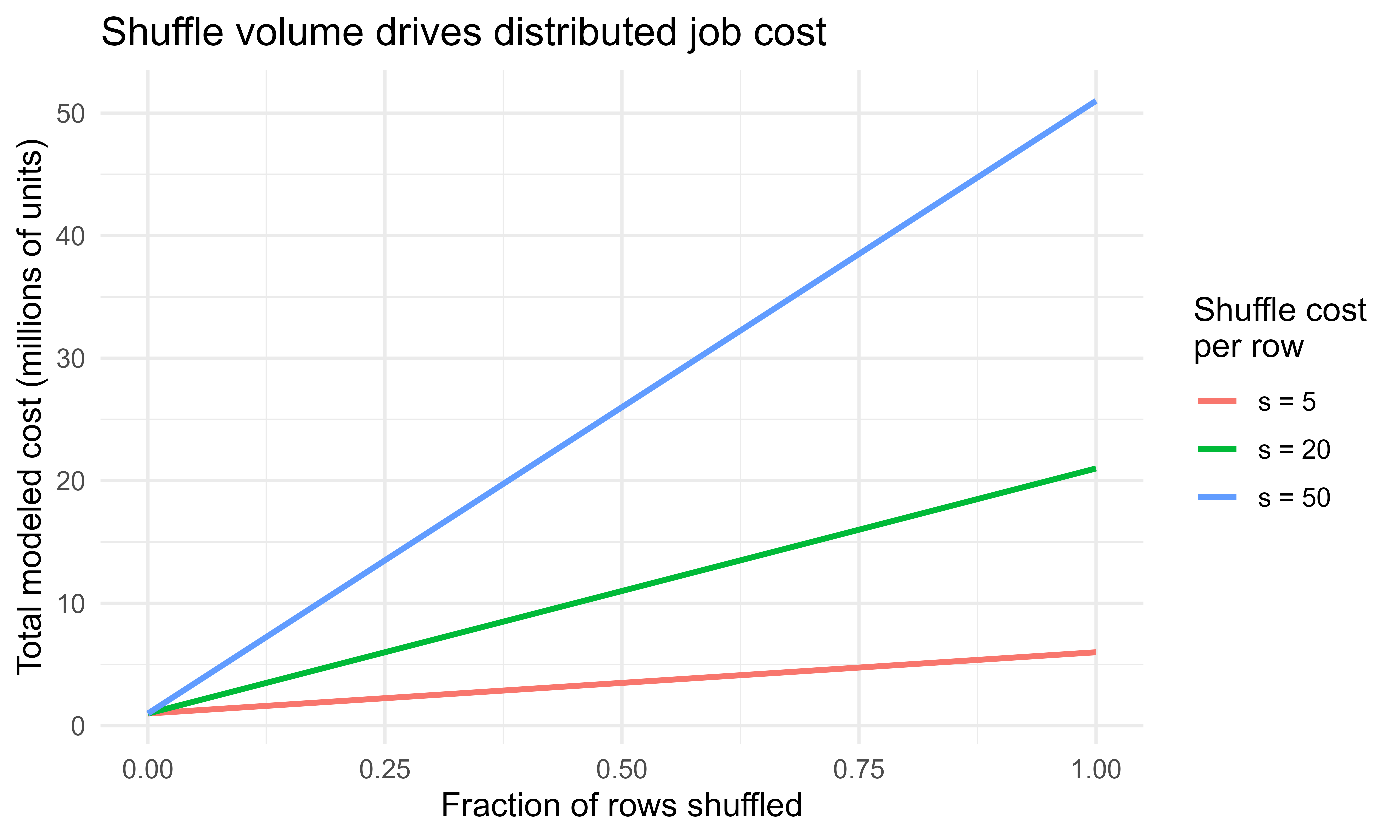
We can now make the cost model from earlier visual. That model said a plan costs roughly $cN + sm$, where $N$ is rows processed, $m$ is rows shuffled, $c$ is per row compute cost, and $s$ is per row shuffle cost with $s \gg c$. Figure 96.1 plots total cost against the fraction of rows shuffled for a fixed $N$, for three values of the shuffle penalty $s$. The steeper the line, the more a small reduction in shuffled rows saves, which is why reducing shuffle (through filtering early, pre-aggregating, and avoiding unnecessary joins and sorts) is where tuning effort pays off.

Show code

library(ggplot2)

N <- 1e6
c_compute <- 1
frac <- seq(0, 1, length.out = 101)

grid <- do.call(rbind, lapply(c(5, 20, 50), function(s) {
  data.frame(
    frac_shuffled = frac,
    total_cost    = c_compute * N + s * (frac * N),
    s_label       = factor(paste0("s = ", s))
  )
}))

ggplot(grid, aes(frac_shuffled, total_cost / 1e6, color = s_label)) +
  geom_line(linewidth = 1) +
  labs(
    x = "Fraction of rows shuffled",
    y = "Total modeled cost (millions of units)",
    color = "Shuffle cost\nper row",
    title = "Shuffle volume drives distributed job cost"
  ) +
  theme_minimal(base_size = 12)

Figure 96.1: Modeled job cost as a function of the fraction of rows shuffled, for compute-cost-per-row c = 1 and three shuffle-cost-per-row values s. When shuffle is much more expensive than compute, the shuffled fraction drives total cost.

96.9 When to use Spark, and when not to

The honest default is: do not use Spark until you need it. Spark adds a cluster, a JVM, network shuffles, and operational overhead, and for data that fits in memory a single machine tool is faster and simpler. Table 96.1 compares the common options for an R user by the data size and setting where each is the right fit.

Table 96.1: Comparison of common tools for an R user by where they run, the data size they suit, their parallelism, and when each is the right choice.

Tool	Where it runs	Good data size	Parallelism	Best when
base R / `dplyr` on a data frame	one R process, one core	fits in RAM	none	data fits in memory and one core is enough
`data.table`	one R process, multi-threaded	fits in RAM	multi-core, in memory	large in memory data, fast joins and aggregations
`multidplyr`	one machine, many R processes	fits across local cores’ memory	multi-core on one box	embarrassingly parallel `dplyr` on one machine
`arrow` / `duckdb`	one machine, out of core	larger than RAM, on local disk	multi-core, streaming	bigger than memory but single machine, columnar files
`sparklyr` / Spark	a cluster (or local Spark)	far larger than one machine	many machines, many cores	data spans machines or lives in a data lake / warehouse

A few rules of thumb summarize the table. If the data fits in RAM, prefer data.table or dplyr; you will not beat them with Spark on one machine. If the data is bigger than RAM but on one machine, try duckdb or arrow (Chapter 100) before reaching for a cluster. Move to Spark when the data is genuinely distributed (many large files in object storage, a warehouse table of billions of rows), when the feature engineering must scan the full table, or when you already operate in a Spark based platform and want to stay in R.

Key idea

Spark earns its overhead only past a size and locality threshold. The right question is not “is my data big?” but “does my data fit on one machine, and if not, where does it already live?” That answer, more than any accuracy concern, decides whether Spark belongs in your pipeline.

96.10 Practical guidance and pitfalls

The pitfalls that bite sparklyr users in practice nearly all trace back to the same root cause: forgetting that the data lives on the cluster and treating a tbl_spark like a local data frame. The following checklist collects the habits that keep that distinction front of mind. Each item is independent, so use it as a reference to return to rather than a sequence to memorize.

Stay lazy, collect late. Build the whole dplyr chain on Spark and call collect() only on a small final result. Calling collect() on a large tbl_spark pulls the entire table into the driver’s R memory and will crash it. When in doubt, sdf_nrow() before you collect.
Read from storage, do not copy_to big data. copy_to() ships data from R into Spark and is only for small reference tables. Large inputs should be read directly with spark_read_parquet, spark_read_csv, and the like, so the data never enters R.
Mind the shuffles. Filter and select before you join or group, so less data moves. Watch for skew, where one key dominates and overloads a single executor; the symptom is one task that runs far longer than the rest.
Set partition count sensibly. Too few partitions underuse the cluster; too many create scheduling overhead and tiny tasks. A common starting point is a small multiple of the total executor cores. Repartition with sdf_repartition() when needed.
Prefer Spark DataFrame ML to round trips. Use ml_* and pipelines so training runs on the cluster. Pulling features into R to fit a local model defeats the purpose and reintroduces the memory limit.
Reproducibility. Set seeds in sdf_random_split() and in MLlib estimators that accept them, and remember that floating point sums can differ slightly with partition count because addition order changes; this is expected, not a bug.
Disconnect. Call spark_disconnect(sc) when finished to release executors, especially on a shared cluster.
Versions matter. Match the sparklyr version, the Spark version, and the cluster’s Spark version; mismatches cause confusing connection and serialization errors. Pin versions in spark_connect(version = ...) and in your environment.

To pull the chapter together: Spark splits data into partitions, runs independent maps on each, and merges the results with associative reduces, moving only small partials across the network. sparklyr lets you drive that machinery from R, translating dplyr verbs into lazy Spark plans and exposing MLlib through the ml_* functions, all without the data ever entering your R session. The base R simulation showed the pattern is nothing mysterious, just partition, map, and combine. And the one rule worth carrying away is the simplest: use Spark when, and only when, the data will not fit on one machine.

96.11 Further reading

Zaharia, M., Chowdhury, M., Das, T., Dave, A., Ma, J., McCauley, M., Franklin, M., Shenker, S., and Stoica, I. (2012). Resilient Distributed Datasets: A Fault-Tolerant Abstraction for In-Memory Cluster Computing. Proceedings of NSDI.
Dean, J. and Ghemawat, S. (2004). MapReduce: Simplified Data Processing on Large Clusters. Proceedings of OSDI.
Armbrust, M., Xin, R., Lian, C., Huai, Y., Liu, D., Bradley, J., Meng, X., Kaftan, T., Franklin, M., Ghodsi, A., and Zaharia, M. (2015). Spark SQL: Relational Data Processing in Spark. Proceedings of SIGMOD.
Meng, X., Bradley, J., Yavuz, B., Sparks, E., Venkataraman, S., Liu, D., et al. (2016). MLlib: Machine Learning in Apache Spark. Journal of Machine Learning Research.
Luraschi, J., Kuo, K., and Ruiz, E. (2019). Mastering Spark with R. O’Reilly Media.
Chambers, B. and Zaharia, M. (2018). Spark: The Definitive Guide. O’Reilly Media.

Spark carries real fixed costs: a Java Virtual Machine, a cluster to manage, network shuffles, and serialization between R and the JVM. On data that fits in memory, a single-machine tool such as data.table will usually finish before Spark has even started its executors.↩︎
Immutability is what makes lineage-based recovery possible. Because a partition is never modified in place, the recipe that built it always reproduces the same result, so Spark can safely recompute a lost partition without worrying that its inputs have since changed.↩︎
Averaging two partition means and then averaging that with a third does not in general equal the overall mean, because the partitions can hold different numbers of rows. Carrying the count alongside the sum repairs this: counts and sums each add associatively, and one final division recovers the correct mean.↩︎
YARN (“Yet Another Resource Negotiator”) is the cluster resource manager that ships with Hadoop; it decides which machines run your executors. On managed platforms such as Databricks or EMR the connection is configured for you and you rarely set master by hand.↩︎

# Distributed Machine Learning with Spark and sparklyr {#sec-spark-sparklyr} ```{r} #| include: false source("_common.R") ``` Apache Spark is an engine for processing data that does not fit on one machine, or that fits but is faster to process across many cores and many machines at once. `sparklyr` is the R interface to Spark: it lets you write `dplyr` verbs and call Spark's machine learning library from an ordinary R session, while the heavy work runs on a cluster. This chapter explains how Spark organizes computation (driver and executors, partitioned data, lazy evaluation), how `sparklyr` connects R to it, how `dplyr` translates to Spark, and how to fit models with Spark MLlib through the `ml_*` functions. Spark is not installed in this environment, so all `sparklyr` and Spark code is marked `eval=FALSE`. The code is written to be correct and current, so you can paste it into a session that has `sparklyr` and a Spark installation. To teach the core computational model with code that actually runs, the chapter includes a base R simulation of the map and reduce pattern (a word count and a partitioned group aggregation) that mirrors what Spark does under the hood. ## Where this fits in a modern workflow Most of the modeling in this book assumes the data sits in memory as a single `data.frame` or `matrix`. That assumption holds for millions of rows but breaks for tens of billions, for data spread across many files in object storage, or for feature engineering that must scan a table far larger than any one machine's RAM. When that happens you have two options: sample the data down until it fits, or push the computation to where the data lives. Spark is the second option. In a typical data and ML pipeline Spark sits at the data preparation and large scale training stage. Raw event logs or transactional records land in a distributed store (a data lake on cloud object storage, or a warehouse table). Spark reads them in parallel, filters and joins and aggregates them into a modeling table, and either trains a model directly with MLlib or writes a manageable extract that a downstream tool consumes. The data engineer often owns the ingestion and transformation; the ML engineer owns the feature pipeline and the model. `sparklyr` lets the R user participate in both without leaving R for SQL or Scala. The decision to use Spark is mostly about data size and where the data already lives, not about model accuracy. A gradient boosting model (@sec-gradient-boosting) on a 10 GB sample will usually predict about as well as the same model on 1 TB; the value of Spark is processing the 1 TB at all when sampling would discard rare but important cases, or when the feature engineering itself requires the full table. ::: {.callout-tip title="When to use this"} Reach for Spark when the data is too large for one machine, is already spread across many files in a data lake or warehouse, or when the feature engineering must scan a table larger than any one machine's RAM. If your data fits comfortably in memory, you almost certainly do not need it.[^spark-overhead] We return to this decision in detail at the end of the chapter. ::: [^spark-overhead]: Spark carries real fixed costs: a Java Virtual Machine, a cluster to manage, network shuffles, and serialization between R and the JVM. On data that fits in memory, a single-machine tool such as `data.table` will usually finish before Spark has even started its executors. ## Spark's computational model ### Driver and executors A Spark application has one driver and many executors. The driver is the process that runs your program: it holds the `SparkContext`, builds the plan of what to compute, and coordinates the work. Executors are worker processes, usually one or more per machine in the cluster, that hold partitions of the data in memory and run the actual computation on them. The driver never touches all the data at once; it sends instructions to executors, and executors return small results (aggregates, counts, model parameters) or write large results to storage. When you run `sparklyr` from R, your R session is the driver side. R talks to the Spark driver (a Java Virtual Machine process) over a connection, the driver distributes tasks to executors, and only summarized results are pulled back into R. This is why you can analyze a table far larger than your laptop's memory: the table never enters R, only the answer does. ::: {.callout-important title="Key idea"} The driver coordinates and the executors compute. Your R session is a thin client that builds a plan and receives small results; the data lives and moves on the cluster. Keeping this picture in mind explains nearly every performance rule later in the chapter. ::: ### Partitions and the RDD The unit of distribution is the partition. A dataset of $N$ rows is split into $P$ partitions, each a contiguous chunk of roughly $N/P$ rows, and each partition is assigned to an executor. A computation over the whole dataset becomes $P$ independent tasks, one per partition, run in parallel across the available cores. The original Spark abstraction for a distributed collection is the Resilient Distributed Dataset (RDD): an immutable, partitioned collection of records together with a record of how it was derived from other datasets. "Resilient" means Spark records the chain of operations (the lineage) that produced each partition, so if an executor dies, Spark recomputes only the lost partitions from their inputs rather than restarting the job.[^rdd-immutable] You rarely use RDDs directly today; the DataFrame is the high level API built on top, a distributed table with named, typed columns. `sparklyr` works almost entirely with Spark DataFrames, which is what makes the `dplyr` translation possible. [^rdd-immutable]: Immutability is what makes lineage-based recovery possible. Because a partition is never modified in place, the recipe that built it always reproduces the same result, so Spark can safely recompute a lost partition without worrying that its inputs have since changed. ::: {.callout-tip title="Intuition"} Think of an RDD's lineage as a cooking recipe rather than a finished dish. If one plate is dropped, you do not redo the whole banquet; you just remake that one plate by following its steps again. ::: ### Transformations, actions, and lazy evaluation Spark operations come in two kinds. Transformations (filter, select, join, group and aggregate) describe a new dataset derived from an existing one. They are lazy: calling them only adds to a plan, the logical plan, and nothing computes yet. Actions (count, collect, write to disk) force the plan to run and produce a result or a side effect. Laziness lets Spark optimize the whole plan before executing. The optimizer (Catalyst) can reorder and combine transformations, push filters down so less data is read, and prune unused columns. The practical consequence in `sparklyr`: a chain of `dplyr` verbs builds a query but does no work until you call something that needs the data, such as `collect()` (pull into R), `sdf_nrow()` (count), or a model fit. If you `collect()` too early, you defeat the optimizer and may pull a huge table into R. ::: {.callout-warning} A common beginner mistake is calling `collect()` partway through a pipeline "to see what is happening." That forces the entire intermediate table into the driver's R memory and can crash the session. Inspect plans with `dplyr::show_query()` or counts with `sdf_nrow()` instead, and `collect()` only the small final result. ::: ### Narrow and wide dependencies Transformations differ in how partitions of the output depend on partitions of the input. A narrow transformation (like a row wise filter or a column computation) lets each output partition be computed from a single input partition, so no data moves between executors. A wide transformation (a group and aggregate, a join, a sort) requires records with the same key to end up on the same executor, which forces a shuffle: data is repartitioned and sent across the network. Shuffles are the expensive part of distributed computing because network and disk are far slower than in memory work. Performance tuning in Spark is largely about reducing the amount of data shuffled and avoiding skew, where one key has far more records than the others and overloads a single executor. The math is simple: if computation cost per row is $c$ and shuffle cost per row is $s$ with $s \gg c$, then a plan that shuffles $m$ rows costs roughly $cN + sm$, and minimizing $m$ dominates. ::: {.callout-tip title="Intuition"} Narrow transformations are like having each worker tidy their own desk: independent and quick. A wide transformation is like asking everyone in the building to sort their papers into shared bins by topic, which means carrying paper down the hall to whoever owns each bin. The hallway traffic, not the sorting, is what slows you down. ::: We make the $cN + sm$ cost model visual in @fig-spark-sparklyr-shuffle-cost near the end of the chapter, after we have seen the map and reduce pattern that produces those shuffles. ## The map and reduce pattern, made precise Spark generalizes the map and reduce model. Two ideas cover most of what executors do. A map applies a function to every record independently. Given a dataset $D = \{x_1, \dots, x_N\}$ partitioned into $D_1, \dots, D_P$, a map with function $g$ produces $\{g(x_1), \dots, g(x_N)\}$, and because $g$ acts on one record at a time, partition $D_j$ can be processed entirely on its own executor with no communication. A reduce combines records with an associative and commutative binary operator $\oplus$ to a single value: $r = x_1 \oplus x_2 \oplus \cdots \oplus x_N$. Associativity and commutativity are what make the reduce parallelizable. Each executor first reduces its own partition locally, $$ r_j = \bigoplus_{x \in D_j} x , $$ and the driver then combines the per partition results, $$ r = r_1 \oplus r_2 \oplus \cdots \oplus r_P . $$ Only the $P$ partial results $r_j$ cross the network, not the $N$ records. This is the structure behind every distributed aggregation. A group and reduce does the same per key: map each record to a key value pair, then reduce the values within each key. The keys force a shuffle so that all values for a key meet on one executor, after which each key is reduced locally. A concrete example: computing a mean. The mean is not associative on its own[^mean-assoc], but the pair (sum, count) is. Each partition emits $(\sum_{x \in D_j} x, |D_j|)$, the partials add componentwise, and the driver divides at the end. Designing an associative combiner like this, so that partition results merge cleanly, is the central skill in writing distributed aggregations, and it is exactly what MLlib does internally to fit models. [^mean-assoc]: Averaging two partition means and then averaging that with a third does not in general equal the overall mean, because the partitions can hold different numbers of rows. Carrying the count alongside the sum repairs this: counts and sums each add associatively, and one final division recovers the correct mean. ::: {.callout-important title="Key idea"} If you can phrase a quantity as the merge of per-partition partial results using an associative, commutative operator, Spark can compute it at scale while moving only the small partials across the network. Most of distributed analytics is finding that associative combiner. ::: ## Connecting R to Spark with sparklyr Now that we understand what Spark is doing under the hood, we can connect R to it. You connect with `spark_connect()`. The `master` argument says where Spark runs: `"local"` starts a single machine Spark on your laptop (useful for development), while a cluster URL or `"yarn"` connects to a real cluster.[^yarn] The returned connection object `sc` is passed to every later call. [^yarn]: YARN ("Yet Another Resource Negotiator") is the cluster resource manager that ships with Hadoop; it decides which machines run your executors. On managed platforms such as Databricks or EMR the connection is configured for you and you rarely set `master` by hand. ::: {.callout-tip} Develop against `master = "local"` on a small sample so your code is fast to iterate, then change a single argument to point at the cluster for the full run. The `sparklyr` code itself does not change between the two. ::: ```{r spark-connect, eval=FALSE} library(sparklyr) library(dplyr) # One time, to install a local Spark for development: # spark_install(version = "3.5") # Local connection for development; use master = "yarn" or a URL on a cluster sc <- spark_connect(master = "local", version = "3.5") # Copy a local data frame into Spark (fine for small data; for big data read # directly from storage instead, see below). The result is a Spark DataFrame # referenced from R by a tbl, not data held in R. cars_tbl <- copy_to(sc, mtcars, name = "cars", overwrite = TRUE) class(cars_tbl) # "tbl_spark": a remote reference, not a local data frame ``` For data of any real size you do not `copy_to` from R; you read it directly into Spark from distributed storage, so the data never passes through R. ```{r spark-read, eval=FALSE} # Read partitioned files straight into Spark. Each file (or block) becomes # one or more partitions, read in parallel by the executors. events <- spark_read_parquet(sc, name = "events", path = "s3a://bucket/events/") trips <- spark_read_csv(sc, name = "trips", path = "/data/trips/*.csv", infer_schema = TRUE, header = TRUE) ``` ## dplyr on Spark The reason `sparklyr` feels natural to an R user is that `dplyr` verbs on a `tbl_spark` are translated to Spark SQL and run on the cluster. You write the same `filter`, `mutate`, `group_by`, and `summarise` you would on a local tibble, and `sparklyr` generates the query. Nothing computes until an action pulls the result. ```{r spark-dplyr, eval=FALSE} summary_tbl <- cars_tbl %>% filter(hp > 100) %>% # narrow: row wise, no shuffle mutate(power_to_weight = hp / wt) %>%# narrow: column computation group_by(cyl) %>% # sets up a wide aggregation summarise( n = n(), mean_mpg = mean(mpg, na.rm = TRUE), mean_ptw = mean(power_to_weight, na.rm = TRUE) ) # still lazy: only a plan so far # See the SQL Spark will run, without running it: dbplyr::sql_render(summary_tbl) # An action. Now Spark executes the plan on the cluster and returns a small # result into R as a local tibble: collected <- summary_tbl %>% collect() ``` The `group_by` then `summarise` is a wide transformation: it shuffles rows so all records for each `cyl` land together, reduces within each group, and returns one row per group. Because the result is small (one row per cylinder count), `collect()` brings back almost nothing. The discipline is: do the shrinking on Spark, `collect()` only what is small. ::: {.callout-note} The `summarise` here is precisely the group-and-reduce from the previous section. `mean(mpg)` is computed as a (sum, count) combiner per `cyl`, merged across partitions, then divided. The `dplyr` verb is a friendly name for the distributed aggregation we worked out by hand. ::: You can also write the result back to storage instead of collecting it, which is what you do when the output is itself large. ```{r spark-write, eval=FALSE} summary_tbl %>% spark_write_parquet(path = "/data/cars_summary/", mode = "overwrite") ``` ## Spark MLlib through the ml_* functions Spark MLlib is Spark's machine learning library. `sparklyr` exposes it through functions prefixed `ml_`, for example `ml_linear_regression`, `ml_logistic_regression`, `ml_random_forest`, `ml_gradient_boosted_trees`, and `ml_kmeans`. These fit models on Spark DataFrames, so training scales across the cluster and the data never enters R. The fitting algorithms are designed for the distributed setting. Linear and logistic regression are trained by iterative optimization where each iteration computes a gradient that is a sum over rows, and that sum is exactly the associative reduce described earlier: each partition computes its partial gradient, the driver adds them, updates the parameters, and broadcasts the new parameters back. For a linear model with parameters $\beta$ and squared error loss, the gradient on the full data is $$ \nabla_\beta \, \mathcal{L}(\beta) = \sum_{i=1}^{N} \nabla_\beta \, \ell\big(y_i, x_i^\top \beta\big) = \sum_{j=1}^{P} \underbrace{\sum_{i \in D_j} \nabla_\beta \, \ell\big(y_i, x_i^\top \beta\big)}_{\text{partial gradient on partition } j} , $$ so each partition produces a partial gradient, and only the $P$ partial gradient vectors (small, of length $p$) are shuffled per iteration, not the $N$ rows. Tree based models distribute differently: they compute split statistics (histograms of features within candidate nodes) per partition and merge those histograms, again an associative combine. ::: {.callout-tip title="Intuition"} Notice that the same trick keeps reappearing. A gradient is a sum over rows, a histogram is a count over rows, a mean is a sum and a count; in every case the per-partition partials are tiny compared to the data, so training a model on a billion rows moves only kilobytes per step. That is why MLlib scales. ::: ```{r spark-mllib, eval=FALSE} # Train / test split done on Spark, never pulling data into R splits <- cars_tbl %>% sdf_random_split(training = 0.7, test = 0.3, seed = 42) fit <- splits$training %>% ml_linear_regression(mpg ~ hp + wt + cyl) summary(fit) # coefficients, R squared, standard errors # Predict on the held out Spark DataFrame; the result is also a Spark DataFrame pred <- ml_predict(fit, splits$test) # Evaluate on Spark, then collect the single number rmse <- ml_regression_evaluator(pred, label_col = "mpg", prediction_col = "prediction", metric_name = "rmse") rmse ``` For multi step feature engineering plus a model, MLlib uses a pipeline: a sequence of stages (transformers that reshape features, and an estimator that learns) fit as one object so the same steps apply identically at training and scoring time. `sparklyr` builds these with `ml_pipeline()`. The functions prefixed `ft_` (for "feature transform") are the reshaping stages: `ft_string_indexer` turns text categories into integer codes, `ft_one_hot_encoder` expands those codes into indicator columns, and `ft_vector_assembler` packs several columns into the single `features` vector that MLlib estimators expect. ::: {.callout-tip} Bundling the preprocessing into the pipeline, rather than doing it ad hoc before the fit, is what guarantees that test data is transformed with the exact rules learned on the training data (the same category-to-index mapping, for instance). This is the distributed analogue of a `recipes` workflow from the tidymodels framework (@sec-tidymodels-framework). ::: ```{r spark-pipeline, eval=FALSE} pipeline <- ml_pipeline(sc) %>% ft_string_indexer(input_col = "category", output_col = "category_idx") %>% ft_one_hot_encoder(input_cols = "category_idx", output_cols = "category_oh") %>% ft_vector_assembler(input_cols = c("hp", "wt", "category_oh"), output_col = "features") %>% ml_logistic_regression(features_col = "features", label_col = "label") model <- ml_fit(pipeline, splits$training) preds <- ml_transform(model, splits$test) # Disconnect when finished to release executors # spark_disconnect(sc) ``` ## A runnable base R simulation of map and reduce All of the `sparklyr` code above needs a Spark installation to run, so it is shown but not executed here. To make the computational model concrete with code that does run, the following chunks use plain base R. They simulate, on a single machine, the partition then map then reduce pattern that Spark distributes across executors. The point is not speed (base R on one core is not fast) but to see the moving parts: data is split into partitions, a map runs independently on each partition, and an associative reduce merges the per partition results. This is exactly the structure MLlib and `dplyr` on Spark rely on; here we play all the roles (driver and executors) ourselves so nothing is hidden. ::: {.callout-note} In a real Spark job the `lapply` calls below would run on different machines in parallel and the merge step would happen after a network shuffle. We use ordinary `lapply` and `rbind` so you can read every step, but the logical structure is identical. ::: First, a distributed word count, the canonical map and reduce example. ```{r mapreduce-wordcount} set.seed(1) # A small "corpus": one string per document docs <- c( "spark splits data into partitions", "each partition is processed by an executor", "map runs on each partition then reduce combines results", "a shuffle moves data so keys meet on one executor", "reduce needs an associative operator to run in parallel" ) # 1. PARTITION: assign documents to P partitions (as Spark splits a dataset) P <- 3 partition_of <- ((seq_along(docs) - 1) %% P) + 1 partitions <- split(docs, partition_of) # 2. MAP (per partition, independent): emit (word, 1) and reduce locally to # per-partition counts. Local pre-aggregation is Spark's "combiner": it # shrinks what must later be shuffled. map_partition <- function(part_docs) { words <- unlist(strsplit(paste(part_docs, collapse = " "), "\\s+")) table(words) # local word counts for this partition } local_counts <- lapply(partitions, map_partition) # 3. SHUFFLE + REDUCE: combine the per-partition tables by key (word). # Addition is associative and commutative, so partial counts merge cleanly. reduce_counts <- function(list_of_tables) { all_words <- sort(unique(unlist(lapply(list_of_tables, names)))) totals <- setNames(numeric(length(all_words)), all_words) for (tab in list_of_tables) { totals[names(tab)] <- totals[names(tab)] + as.numeric(tab) } totals } word_counts <- reduce_counts(local_counts) head(sort(word_counts, decreasing = TRUE), 6) ``` Next, a partitioned group aggregation that computes a group mean the distributed way, using the (sum, count) combiner so the merge across partitions is associative. We also check the result against a single machine computation to confirm the distributed pattern gives the identical answer. ```{r mapreduce-groupmean} set.seed(42) N <- 100000 dat <- data.frame( key = sample(letters[1:5], N, replace = TRUE), value = rnorm(N, mean = 10, sd = 3) ) # PARTITION the rows across P executors P <- 8 dat$part <- sample(seq_len(P), N, replace = TRUE) parts <- split(dat[c("key", "value")], dat$part) # MAP + local REDUCE: per partition, compute partial (sum, count) per key. # (sum, count) is the associative combiner that makes the mean parallelizable. map_local_agg <- function(df) { s <- tapply(df$value, df$key, sum) n <- tapply(df$value, df$key, length) data.frame(key = names(s), sum = as.numeric(s), n = as.numeric(n)) } partials <- lapply(parts, map_local_agg) # SHUFFLE + REDUCE: stack the partials and add sums and counts within each key, # then divide once at the end. Only P small tables are merged, not N rows. all_partials <- do.call(rbind, partials) merged <- aggregate(cbind(sum, n) ~ key, data = all_partials, FUN = sum) merged$mean <- merged$sum / merged$n # Verify against the single-machine answer single <- aggregate(value ~ key, data = dat, FUN = mean) compare <- merge(merged[c("key", "mean")], single, by = "key") names(compare) <- c("key", "distributed_mean", "single_machine_mean") compare$max_abs_diff <- abs(compare$distributed_mean - compare$single_machine_mean) compare ``` The `max_abs_diff` column is essentially zero (differences at the level of floating point rounding), which is the whole point: a correctly designed associative combiner makes the distributed computation produce the same result as the single machine computation, while only small partial results cross between partitions. ::: {.callout-warning} "Essentially zero" is not always "exactly zero." Because floating point addition is not perfectly associative, summing the same numbers in a different order (as happens when the partition count changes) can shift the last digits. This is expected behavior, not a bug, and is why distributed sums are reproducible only when the partitioning is fixed. ::: ## A figure: why shuffle volume dominates cost We can now make the cost model from earlier visual. That model said a plan costs roughly $cN + sm$, where $N$ is rows processed, $m$ is rows shuffled, $c$ is per row compute cost, and $s$ is per row shuffle cost with $s \gg c$. @fig-spark-sparklyr-shuffle-cost plots total cost against the fraction of rows shuffled for a fixed $N$, for three values of the shuffle penalty $s$. The steeper the line, the more a small reduction in shuffled rows saves, which is why reducing shuffle (through filtering early, pre-aggregating, and avoiding unnecessary joins and sorts) is where tuning effort pays off. ```{r fig-spark-sparklyr-shuffle-cost, fig.width=7, fig.height=4.2, fig.cap="Modeled job cost as a function of the fraction of rows shuffled, for compute-cost-per-row c = 1 and three shuffle-cost-per-row values s. When shuffle is much more expensive than compute, the shuffled fraction drives total cost."} library(ggplot2) N <- 1e6 c_compute <- 1 frac <- seq(0, 1, length.out = 101) grid <- do.call(rbind, lapply(c(5, 20, 50), function(s) { data.frame( frac_shuffled = frac, total_cost = c_compute * N + s * (frac * N), s_label = factor(paste0("s = ", s)) ) })) ggplot(grid, aes(frac_shuffled, total_cost / 1e6, color = s_label)) + geom_line(linewidth = 1) + labs( x = "Fraction of rows shuffled", y = "Total modeled cost (millions of units)", color = "Shuffle cost\nper row", title = "Shuffle volume drives distributed job cost" ) + theme_minimal(base_size = 12) ``` ## When to use Spark, and when not to The honest default is: do not use Spark until you need it. Spark adds a cluster, a JVM, network shuffles, and operational overhead, and for data that fits in memory a single machine tool is faster and simpler. @tbl-spark-sparklyr-tool-comparison compares the common options for an R user by the data size and setting where each is the right fit. | Tool | Where it runs | Good data size | Parallelism | Best when | |---|---|---|---|---| | base R / `dplyr` on a data frame | one R process, one core | fits in RAM | none | data fits in memory and one core is enough | | `data.table` | one R process, multi-threaded | fits in RAM | multi-core, in memory | large in memory data, fast joins and aggregations | | `multidplyr` | one machine, many R processes | fits across local cores' memory | multi-core on one box | embarrassingly parallel `dplyr` on one machine | | `arrow` / `duckdb` | one machine, out of core | larger than RAM, on local disk | multi-core, streaming | bigger than memory but single machine, columnar files | | `sparklyr` / Spark | a cluster (or local Spark) | far larger than one machine | many machines, many cores | data spans machines or lives in a data lake / warehouse | : Comparison of common tools for an R user by where they run, the data size they suit, their parallelism, and when each is the right choice. {#tbl-spark-sparklyr-tool-comparison} A few rules of thumb summarize the table. If the data fits in RAM, prefer `data.table` or `dplyr`; you will not beat them with Spark on one machine. If the data is bigger than RAM but on one machine, try `duckdb` or `arrow` (@sec-duckdb-arrow) before reaching for a cluster. Move to Spark when the data is genuinely distributed (many large files in object storage, a warehouse table of billions of rows), when the feature engineering must scan the full table, or when you already operate in a Spark based platform and want to stay in R. ::: {.callout-important title="Key idea"} Spark earns its overhead only past a size and locality threshold. The right question is not "is my data big?" but "does my data fit on one machine, and if not, where does it already live?" That answer, more than any accuracy concern, decides whether Spark belongs in your pipeline. ::: ## Practical guidance and pitfalls The pitfalls that bite `sparklyr` users in practice nearly all trace back to the same root cause: forgetting that the data lives on the cluster and treating a `tbl_spark` like a local data frame. The following checklist collects the habits that keep that distinction front of mind. Each item is independent, so use it as a reference to return to rather than a sequence to memorize. - Stay lazy, collect late. Build the whole `dplyr` chain on Spark and call `collect()` only on a small final result. Calling `collect()` on a large `tbl_spark` pulls the entire table into the driver's R memory and will crash it. When in doubt, `sdf_nrow()` before you collect. - Read from storage, do not `copy_to` big data. `copy_to()` ships data from R into Spark and is only for small reference tables. Large inputs should be read directly with `spark_read_parquet`, `spark_read_csv`, and the like, so the data never enters R. - Mind the shuffles. Filter and select before you join or group, so less data moves. Watch for skew, where one key dominates and overloads a single executor; the symptom is one task that runs far longer than the rest. - Set partition count sensibly. Too few partitions underuse the cluster; too many create scheduling overhead and tiny tasks. A common starting point is a small multiple of the total executor cores. Repartition with `sdf_repartition()` when needed. - Prefer Spark DataFrame ML to round trips. Use `ml_*` and pipelines so training runs on the cluster. Pulling features into R to fit a local model defeats the purpose and reintroduces the memory limit. - Reproducibility. Set seeds in `sdf_random_split()` and in MLlib estimators that accept them, and remember that floating point sums can differ slightly with partition count because addition order changes; this is expected, not a bug. - Disconnect. Call `spark_disconnect(sc)` when finished to release executors, especially on a shared cluster. - Versions matter. Match the `sparklyr` version, the Spark version, and the cluster's Spark version; mismatches cause confusing connection and serialization errors. Pin versions in `spark_connect(version = ...)` and in your environment. To pull the chapter together: Spark splits data into partitions, runs independent maps on each, and merges the results with associative reduces, moving only small partials across the network. `sparklyr` lets you drive that machinery from R, translating `dplyr` verbs into lazy Spark plans and exposing MLlib through the `ml_*` functions, all without the data ever entering your R session. The base R simulation showed the pattern is nothing mysterious, just partition, map, and combine. And the one rule worth carrying away is the simplest: use Spark when, and only when, the data will not fit on one machine. ## Further reading - Zaharia, M., Chowdhury, M., Das, T., Dave, A., Ma, J., McCauley, M., Franklin, M., Shenker, S., and Stoica, I. (2012). Resilient Distributed Datasets: A Fault-Tolerant Abstraction for In-Memory Cluster Computing. Proceedings of NSDI. - Dean, J. and Ghemawat, S. (2004). MapReduce: Simplified Data Processing on Large Clusters. Proceedings of OSDI. - Armbrust, M., Xin, R., Lian, C., Huai, Y., Liu, D., Bradley, J., Meng, X., Kaftan, T., Franklin, M., Ghodsi, A., and Zaharia, M. (2015). Spark SQL: Relational Data Processing in Spark. Proceedings of SIGMOD. - Meng, X., Bradley, J., Yavuz, B., Sparks, E., Venkataraman, S., Liu, D., et al. (2016). MLlib: Machine Learning in Apache Spark. Journal of Machine Learning Research. - Luraschi, J., Kuo, K., and Ruiz, E. (2019). Mastering Spark with R. O'Reilly Media. - Chambers, B. and Zaharia, M. (2018). Spark: The Definitive Guide. O'Reilly Media.