Advanced Data Analysis

Nguyen, Mike

4 Kernel Smoothing

Suppose you want to draw a smooth curve through a scatterplot, but you are not willing to commit to a global shape like a straight line or a polynomial. A natural instinct is to look at each point on the x-axis and ask: what is the average response among the observations that sit nearby? Slide that local average across the range of $x$ and you trace out a flexible curve. Kernel smoothing (also called kernel regression) turns this instinct into a precise method.

The central idea is to fit a separate but very simple model at each query point $x_0$, using only the observations that are “close” to $x_0$. Closeness is measured by a weighting function, also called a kernel, written $K_\lambda(x_0, x_i)$. The kernel assigns a large weight to observations near $x_0$ and a small (or zero) weight to those far away. Because the weights change smoothly as $x_0$ moves, the resulting estimate $\hat{f}(x)$ is itself smooth across the input space $R^p$.

Intuition

A kernel is just a recipe for “how much should this neighbor count?” Points right next to $x_0$ get a full vote, points a little further away get a fractional vote, and points beyond the kernel’s reach get no vote at all.

The kernel carries a parameter $\lambda$ that sets the “width” of the neighborhood, that is, how far away an observation can be and still influence the fit. Choosing $\lambda$ is the main modeling decision in kernel smoothing, which is one of its appeals: there is very little to train. The cost shows up at prediction time instead. Kernel smoothers are memory-based methods, meaning the entire training set must be kept around and consulted every time we want a prediction at a new location $x_0$.¹

In this chapter you will learn how a kernel turns nearby observations into a local estimate, the common choices of kernel and how they differ, how the width $\lambda$ trades bias against variance, and how the same kernel machinery can estimate a probability density rather than a regression function. Kernel smoothing sits between the rigidity of global parametric models and the full flexibility of methods like local regression (Chapter 5), which builds directly on the ideas here.

4.1 One-Dimensional Kernel Smoothers

To see what a kernel buys us, start from a method you may already know: $k$-nearest neighbors (Chapter 17). The $k$-NN estimate at a point $x$ is simply the average response over the $k$ observations closest to $x$,

\[ \hat{f}(x) = Ave (y_i |x_i \in N_k(x)) \]

where $N_k(x)$ refers to the set of $k$ neighbors nearest the point $x$ in squared distance. This works, but it has an awkward feature: as $x$ slides along, observations pop in and out of the neighborhood one at a time, so the fitted curve jumps at each switch. The estimate is a step function, not a smooth one.

The fix is to stop treating neighbors as “in or out” and instead weight them continuously by distance. This gives the Nadaraya-Watson kernel-weighted average,

\[ \hat{f}(x_0)= \frac{\sum_{i=1}^n K_\lambda(x_0,x_i) y_i}{\sum_{i=1}^n K_\lambda(x_0, x_i)} \]

where the kernel is defined through a function $D$ applied to the scaled distance,

\[ K_\lambda(x_0,x) = D(\frac{|x-x_0|}{\lambda}) \]

Read the formula as a weighted average: each $y_i$ is multiplied by its weight $K_\lambda(x_0, x_i)$, and the denominator normalizes the weights so they sum to one. The key difference from nearest neighbors is that the weights now change continuously as $x_0$ moves, rather than in discrete jumps. The result is a smooth curve, which is both more pleasant to look at and, in some settings, more useful to work with.

Key idea

Nearest neighbors gives every neighbor an equal vote and everyone else zero. A kernel replaces that hard cutoff with a smooth falloff in influence, and smoothness in the weights produces smoothness in the fit.

4.1.1 The Nadaraya-Watson estimator as a local average

The Nadaraya-Watson estimator is not an arbitrary recipe: it is the solution of a weighted least squares problem, and it is the natural plug-in estimator for the conditional mean. Both views are worth making precise.

Assume the data $(x_i, y_i)_{i=1}^n$ are an i.i.d. sample from a joint distribution with density $f_{X,Y}$, and write the regression function as the conditional mean \[ f(x_0) = \mathbb{E}[Y \mid X = x_0] = \int y \, \frac{f_{X,Y}(x_0, y)}{f_X(x_0)} \, dy = \frac{\int y \, f_{X,Y}(x_0, y)\, dy}{f_X(x_0)}. \]

Replace the unknown joint and marginal densities by kernel density estimates. With a kernel $K_\lambda(x_0, x) = \lambda^{-1} D(|x - x_0|/\lambda)$ and a product kernel in $(x, y)$, the estimates are \[ \hat f_X(x_0) = \frac{1}{n}\sum_{i=1}^n K_\lambda(x_0, x_i), \qquad \widehat{f_{X,Y}}(x_0, y) = \frac{1}{n}\sum_{i=1}^n K_\lambda(x_0, x_i)\, K_h(y, y_i). \] Substituting and using $\int y\, K_h(y, y_i)\, dy = y_i$ (any kernel that is a symmetric density centered at $y_i$ has mean $y_i$, so the bandwidth $h$ cancels) gives \[ \hat f(x_0) = \frac{\frac{1}{n}\sum_i K_\lambda(x_0, x_i)\, y_i}{\frac{1}{n}\sum_i K_\lambda(x_0, x_i)} = \frac{\sum_{i=1}^n K_\lambda(x_0, x_i)\, y_i}{\sum_{i=1}^n K_\lambda(x_0, x_i)}. \tag{4.1}\] This is exactly the Nadaraya-Watson average. The derivation shows the estimator is the conditional mean computed under the kernel density estimate of the data, which is why it inherits both the strengths (consistency) and the weaknesses (boundary bias) of kernel density estimation.

Equivalently, $\hat f(x_0)$ is the constant $\beta_0$ that minimizes the locally weighted sum of squares \[ \hat f(x_0) = \arg\min_{\beta_0} \sum_{i=1}^n K_\lambda(x_0, x_i)\,(y_i - \beta_0)^2 . \tag{4.2}\] Setting the derivative with respect to $\beta_0$ to zero gives $\sum_i K_\lambda(x_0,x_i)(y_i - \beta_0) = 0$, whose solution is the weighted average in Equation 4.1. Reading the estimator this way, as fitting a local constant, makes it clear what local regression (Chapter 5) changes: it replaces the local constant $\beta_0$ by a local line or polynomial, which is what removes the boundary bias discussed below.

4.1.2 The estimator is linear in the responses

A fact that drives all of the theory is that the fit is linear in $y$. Define the equivalent kernel weights \[ \ell_i(x_0) = \frac{K_\lambda(x_0, x_i)}{\sum_{j=1}^n K_\lambda(x_0, x_j)}, \qquad \hat f(x_0) = \sum_{i=1}^n \ell_i(x_0)\, y_i , \tag{4.3}\] where the weights satisfy $\sum_i \ell_i(x_0) = 1$ for every $x_0$ but in general $\sum_i x_i \,\ell_i(x_0) \neq x_0$. Stacking the fitted values at the training points gives $\hat{\mathbf{y}} = \mathbf{S}\,\mathbf{y}$ with smoother matrix $S_{ij} = \ell_j(x_i)$. Because $\mathbf S$ does not depend on $\mathbf y$, the kernel smoother is a linear smoother, exactly like ridge or spline smoothers, and the effective degrees of freedom of the fit can be defined as $\mathrm{df}_\lambda = \operatorname{tr}(\mathbf S)$. This single number summarizes complexity across kernels and bandwidths and is what makes different smoothers comparable: a kernel fit with $\operatorname{tr}(\mathbf S) = 8$ is roughly as flexible as a degree-$7$ polynomial regression.

4.1.3 Choosing the kernel function

The shape of $D$ determines how influence falls off with distance. Three choices are standard, and they differ mainly in how abruptly the weight drops to zero and how smooth they are at their edges.

The Epanechnikov quadratic kernel is compact, meaning it gives exactly zero weight beyond a finite radius:

\[ D(t) = \begin{cases} \frac{3}{4}(1-t^2) & \text{if } |t| \le 1 \\ 0 & \text{otherwise} \end{cases} \]

It is computationally cheap because most observations contribute nothing, but it has no continuous derivative at the boundary of its support, so the fitted curve can show small kinks.

The tri-cube kernel is also compact but smoother, with two continuous derivatives at the boundary of its support:

\[ D(t) = \begin{cases} (1- |t|^3)^3 & \text{if } |t| \le 1 \\ 0 & \text{otherwise} \end{cases} \]

where $t = |x - x_0|/\lambda$ (the same scaled argument used for every kernel). The extra smoothness at the edges makes it a popular default for local regression.

The Gaussian density uses the familiar bell curve as the weighting function:

\[ D(t) = \frac{\exp(-\frac{t^2}{2\sigma^2})}{\sqrt{2 \pi}\sigma} \]

where $\sigma$ plays the role of the “width.” It is continuously differentiable everywhere, which is attractive, but it has infinite support: every observation gets a nonzero weight, however tiny. That can make it more taxing to compute on large data sets, since no point can be skipped.

Tip

When you need a smooth fit and computation is not a bottleneck, a Gaussian or tri-cube kernel is a safe choice. When the data set is large and you want speed, prefer a compact kernel like the Epanechnikov or tri-cube so that distant points can be ignored entirely.

So far $\lambda$ has been a single fixed number, but the neighborhood width need not be constant. With adaptive neighborhoods, the width depends on the location $x_0$,

\[ K_\lambda (x_0, x) = D(\frac{|x-x_0|}{h_\lambda(x_0)}) \]

so the kernel can widen in sparse regions and tighten where data are plentiful.

A few consequences of these choices are worth keeping in mind:

A large $\lambda$ lowers variance, because we average over more observations (effectively a larger $n$), but it raises bias, because we approximate $f(x_0)$ using observations that lie further from $x_0$.
An adaptive width $h_\lambda(x)$ can hold the bias roughly constant across the input space, but then the variance becomes inversely proportional to the local density of observations: where data are sparse, the estimate is noisier.
The biggest weakness of kernel smoothers is estimation near the boundaries of the data. Near an edge the kernel becomes lopsided, with neighbors on only one side, so the fit is badly biased there. Local regression (Chapter 5) was designed partly to correct this boundary bias.

Warning

Trust a kernel smoother least at the left and right ends of the data. The asymmetry of the neighborhood near a boundary systematically pulls the fit toward the interior, and no amount of width tuning fully removes it.

4.2 Selecting the Kernel Width

Everything above turns on one number, $\lambda$, the width of the kernel $K_\lambda$. Its precise meaning depends on which kernel you chose:

For the Epanechnikov and tri-cube kernels, $\lambda$ is the radius of the support region, that is, the distance beyond which weights are zero.
For the Gaussian kernel, $\lambda$ is the standard deviation $\sigma$.
For the nearest-neighbor smoother, the role of $\lambda$ is played by $k$, the number of neighbors.

In every case the qualitative tradeoff is the same. A smaller width does less averaging, giving higher variance but smaller bias (the fit tracks local wiggles, including noise). A larger width does more averaging, giving lower variance but higher bias (the fit is smoother but can miss real structure). This is the bias-variance tradeoff in its most visible form: $\lambda$ is the dial between an overly jagged fit and an overly flat one.

When to use this

Reach for kernel smoothing when you want a flexible one-dimensional (or low-dimensional) curve, you have enough data to average locally, and you care more about following the data’s shape than about an interpretable equation.

Because there is no formula that hands you the right width, $\lambda$ is chosen by data-driven tuning, most commonly [Cross-validation]: try a grid of widths, estimate out-of-sample error for each, and keep the width that minimizes it.

4.2.1 The bias-variance tradeoff, made precise

The qualitative statements above can be turned into formulas, and the formulas tell you the optimal bandwidth and the best achievable error rate. Work in one dimension with equally weighted data of size $n$, a kernel that is a symmetric density with \[ \int D(u)\, du = 1, \quad \int u\, D(u)\, du = 0, \quad \mu_2 = \int u^2 D(u)\, du, \quad R(D) = \int D(u)^2\, du, \] and suppose $f$ is twice continuously differentiable and the design density $g(x)$ is smooth and bounded away from zero near $x_0$. As $n \to \infty$ and $\lambda \to 0$ with $n\lambda \to \infty$, a Taylor expansion of the Nadaraya-Watson estimator gives the standard asymptotic moments at an interior point: \[ \operatorname{Bias}\!\big(\hat f(x_0)\big) \approx \tfrac{1}{2}\lambda^2 \mu_2 \left[ f''(x_0) + \frac{2 f'(x_0) g'(x_0)}{g(x_0)} \right], \tag{4.4}\] \[ \operatorname{Var}\!\big(\hat f(x_0)\big) \approx \frac{\sigma^2 R(D)}{n \lambda\, g(x_0)}, \tag{4.5}\] where $\sigma^2 = \operatorname{Var}(Y \mid X = x_0)$. Two structural facts are visible immediately. First, the bias grows like $\lambda^2$ (wider kernel, more averaging over curvature) while the variance shrinks like $1/(n\lambda)$ (wider kernel averages more points), so the two genuinely pull in opposite directions. Second, the variance is inversely proportional to the local design density $g(x_0)$: where data are sparse the estimate is noisier, which is the formal version of the adaptive-width remark in Chapter 4.

The design-density term $2 f' g'/g$ in Equation 4.4 is the design bias of the local-constant fit. It does not vanish even where $f$ is linear, and it is exactly the term that local linear regression (Chapter 5) annihilates, which is the precise reason local regression is preferred at boundaries and in regions of changing density.

Minimizing the asymptotic mean squared error $\operatorname{MSE} = \operatorname{Bias}^2 + \operatorname{Var}$ over $\lambda$ gives the optimal local bandwidth. Writing $b(x_0)$ for the bracketed curvature term in Equation 4.4, $\operatorname{MSE}(\lambda) \approx \tfrac14 \lambda^4 \mu_2^2 b(x_0)^2 + \sigma^2 R(D)/(n\lambda g(x_0))$; differentiating and setting to zero, \[ \lambda_{\text{opt}}(x_0) = \left[ \frac{\sigma^2 R(D)}{\mu_2^2\, b(x_0)^2\, g(x_0)} \right]^{1/5} n^{-1/5}, \qquad \operatorname{MSE}\big(\lambda_{\text{opt}}\big) = O\!\left(n^{-4/5}\right). \tag{4.6}\] This is the canonical rate for one-dimensional nonparametric smoothing: the best bandwidth shrinks like $n^{-1/5}$ and the pointwise error converges at $n^{-4/5}$, strictly slower than the $n^{-1}$ MSE of a correctly specified parametric model. That gap is the price of not committing to a global form, and it cannot be beaten without extra smoothness assumptions on $f$.

Curse of dimensionality

In $p$ dimensions with a product kernel the same expansion gives bias $O(\lambda^2)$ and variance $O\!\big(1/(n\lambda^p)\big)$, so the optimal bandwidth is $\lambda_{\text{opt}} \propto n^{-1/(p+4)}$ and the optimal MSE is $O\!\big(n^{-4/(p+4)}\big)$. The rate degrades sharply with $p$: matching the accuracy a one-dimensional smoother reaches with $n$ points requires roughly $n^{(p+4)/5}$ points in $p$ dimensions. This is why raw kernel smoothing is a low-dimensional tool, and why high-dimensional problems call for structure such as additivity (Chapter 6) or projection.

4.2.2 Practical bandwidth selection

In practice three routes to a bandwidth are common, in increasing order of robustness.

Leave-one-out cross-validation, computed cheaply. Because the smoother is linear (Equation 4.3), the leave-one-out residual has a closed form that avoids refitting $n$ times. If $S_{ii}$ is the $i$th diagonal of the smoother matrix, then \[ y_i - \hat f^{(-i)}(x_i) = \frac{y_i - \hat f(x_i)}{1 - S_{ii}}, \qquad \operatorname{CV}(\lambda) = \frac{1}{n}\sum_{i=1}^n \left( \frac{y_i - \hat f(x_i)}{1 - S_{ii}} \right)^2 , \tag{4.7}\] so a full LOOCV curve costs one fit per candidate $\lambda$, not $n$. The same identity underlies generalized cross-validation, which replaces $S_{ii}$ by the average $\operatorname{tr}(\mathbf S)/n$.

Plug-in rules. Equation 4.6 depends only on $\sigma^2$, the design density, and the curvature functional $\int b(x)^2 g(x)\, dx$. Plug-in methods estimate these from a pilot fit and substitute them, giving a bandwidth without a search. They converge faster than cross-validation but require the smoothness assumptions to hold.

Rules of thumb (density estimation). For Gaussian KDE of a roughly Gaussian sample, Silverman’s rule sets $\lambda = 0.9\, \min(\hat\sigma, \widehat{\mathrm{IQR}}/1.34)\, n^{-1/5}$, which minimizes asymptotic integrated squared error under normality and is the default in density(). It oversmooths multimodal densities, so treat it as a starting point and reduce $\lambda$ if structure is suspected.

The leave-one-out shortcut in Equation 4.7 is worth checking directly: the closed-form residual should equal an honest refit that deletes each point. The following base R simulation confirms it for a Gaussian Nadaraya-Watson smoother.

Show code

set.seed(1)
n <- 40
x <- sort(runif(n)); y <- sin(2 * pi * x) + rnorm(n, sd = 0.2)
lambda <- 0.1

# Smoother matrix S with row-normalized Gaussian weights
W <- outer(x, x, function(a, b) dnorm((a - b) / lambda))
S <- W / rowSums(W)
fit <- as.vector(S %*% y)

# Closed-form LOO residuals via the diagonal of S
loo_closed <- (y - fit) / (1 - diag(S))

# Brute-force LOO: delete each point and refit
loo_brute <- sapply(seq_len(n), function(i) {
  w <- dnorm((x[i] - x[-i]) / lambda)
  y[i] - sum(w * y[-i]) / sum(w)
})

max(abs(loo_closed - loo_brute))  # ~ 0 up to floating point
#> [1] 3.851086e-16

A useful diagnostic across all routes: plot the fit at several bandwidths spanning the cross-validation minimum. A good $\lambda$ sits in a region where the fit is visually stable; if the curve changes character drastically for small changes in $\lambda$, the data do not pin the bandwidth down and the smoothest defensible choice should be preferred.

Failure modes

Kernel smoothers break in predictable ways: (i) at boundaries, where the one-sided neighborhood induces $O(\lambda)$ bias rather than $O(\lambda^2)$, fixed only by local polynomials; (ii) under heteroscedastic or heavy-tailed noise, where the local average is not robust and a single outlier drags the fit; (iii) in regions of sharply varying density, where a global bandwidth is simultaneously too wide where data are dense and too narrow where data are sparse; and (iv) in moderate to high dimension, where the curse of dimensionality empties every neighborhood.

4.3 Kernel Density Estimation

Kernels did not begin as a regression tool. Their original job was to estimate a probability density, and that use is still common today. The shift in goal is small: instead of averaging response values $y_i$ near $x_0$, we count how many observations pile up near $x_0$, which tells us how probable that region is.

Suppose we have a random sample $x_1, \dots, x_n$ drawn from an unknown probability density $f_X(x)$, and we want to estimate $f_X$ at a point $x_0$, working in one dimension so $X \in R$. The Parzen estimate places a small kernel bump at every observation and adds them up:

\[ \hat{f}_X(x_0) = \frac{1}{n \lambda}\sum_{i=1}^n K_\lambda (x_0, x_i) \]

A common choice is the Gaussian kernel with standard deviation $\lambda$. The leading factor $\frac{1}{n\lambda}$ normalizes the result so that it integrates to one, as a density must. The same construction extends to higher dimensions by replacing the one-dimensional kernel with a multivariate (Gaussian) kernel.

Intuition

Picture dropping a tiny mound of sand on the number line at each data point. Where points cluster, the mounds overlap and pile high; where points are scarce, the sand is thin. The resulting profile, rescaled to integrate to one, is the estimated density.

4.3.1 Bias, variance, and the optimal density bandwidth

The same expansion that governed regression applies to the density estimate, and here it is cleaner because there is no design density to contend with. Write the estimator with a kernel $D$ that is a symmetric density as $\hat f_X(x_0) = \tfrac{1}{n\lambda}\sum_i D\!\big((x_0 - x_i)/\lambda\big)$. Taking the expectation over one observation, \[ \mathbb{E}\,\hat f_X(x_0) = \frac{1}{\lambda}\int D\!\Big(\frac{x_0 - u}{\lambda}\Big) f_X(u)\, du = \int D(t)\, f_X(x_0 - \lambda t)\, dt , \] and a second-order Taylor expansion $f_X(x_0 - \lambda t) = f_X(x_0) - \lambda t f_X'(x_0) + \tfrac12 \lambda^2 t^2 f_X''(x_0) + o(\lambda^2)$, together with $\int D = 1$ and $\int t D(t)\, dt = 0$, yields \[ \operatorname{Bias}\!\big(\hat f_X(x_0)\big) \approx \tfrac{1}{2}\lambda^2 \mu_2\, f_X''(x_0), \qquad \operatorname{Var}\!\big(\hat f_X(x_0)\big) \approx \frac{f_X(x_0)\, R(D)}{n\lambda} . \tag{4.8}\] The bias is proportional to the curvature $f_X''$: a Gaussian KDE flattens peaks and fills valleys, the same oversmoothing that Silverman’s rule risks. Integrating the mean squared error over $x_0$ gives the asymptotic mean integrated squared error, \[ \operatorname{AMISE}(\lambda) = \frac{R(D)}{n\lambda} + \frac{1}{4}\lambda^4 \mu_2^2 \int f_X''(x)^2\, dx , \] and minimizing over $\lambda$ gives the optimal density bandwidth and rate, \[ \lambda_{\text{opt}} = \left[ \frac{R(D)}{\mu_2^2 \int (f_X'')^2}\right]^{1/5} n^{-1/5}, \qquad \operatorname{AMISE}\big(\lambda_{\text{opt}}\big) = O\!\left(n^{-4/5}\right). \tag{4.9}\] The $n^{-1/5}$ bandwidth and $n^{-4/5}$ error mirror the regression case, and substituting the standard normal for $f_X$ and the Gaussian for $D$ in Equation 4.9 reproduces Silverman’s rule exactly.

Density estimates are not only descriptive: they plug directly into classification through Bayes’ theorem. Suppose there are $J$ classes, and we fit a separate nonparametric density $\hat{f}_j (X)$ for $j = 1, \dots, J$, one per class. Given a prior probability $\hat{\pi}_j$ for each class (these might come from the observed class proportions or from outside knowledge), the posterior probability that a new point $x_0$ belongs to class $j$ is

\[ \hat{P}(G=j | X=x_0) = \frac{\hat{\pi}_j \hat{f}_j (x_0)}{\sum_{k=1}^J \hat{\pi}_k \hat{f}_k (x_0)} \]

In words, we weight each class density by its prior and renormalize across classes, then assign $x_0$ to whichever class comes out largest. This is the kernel-based cousin of methods like the naive Bayes (Chapter 18) and discriminant (Chapter 20) classifiers.

4.4 Kernel Smoothing in R: A Worked Example

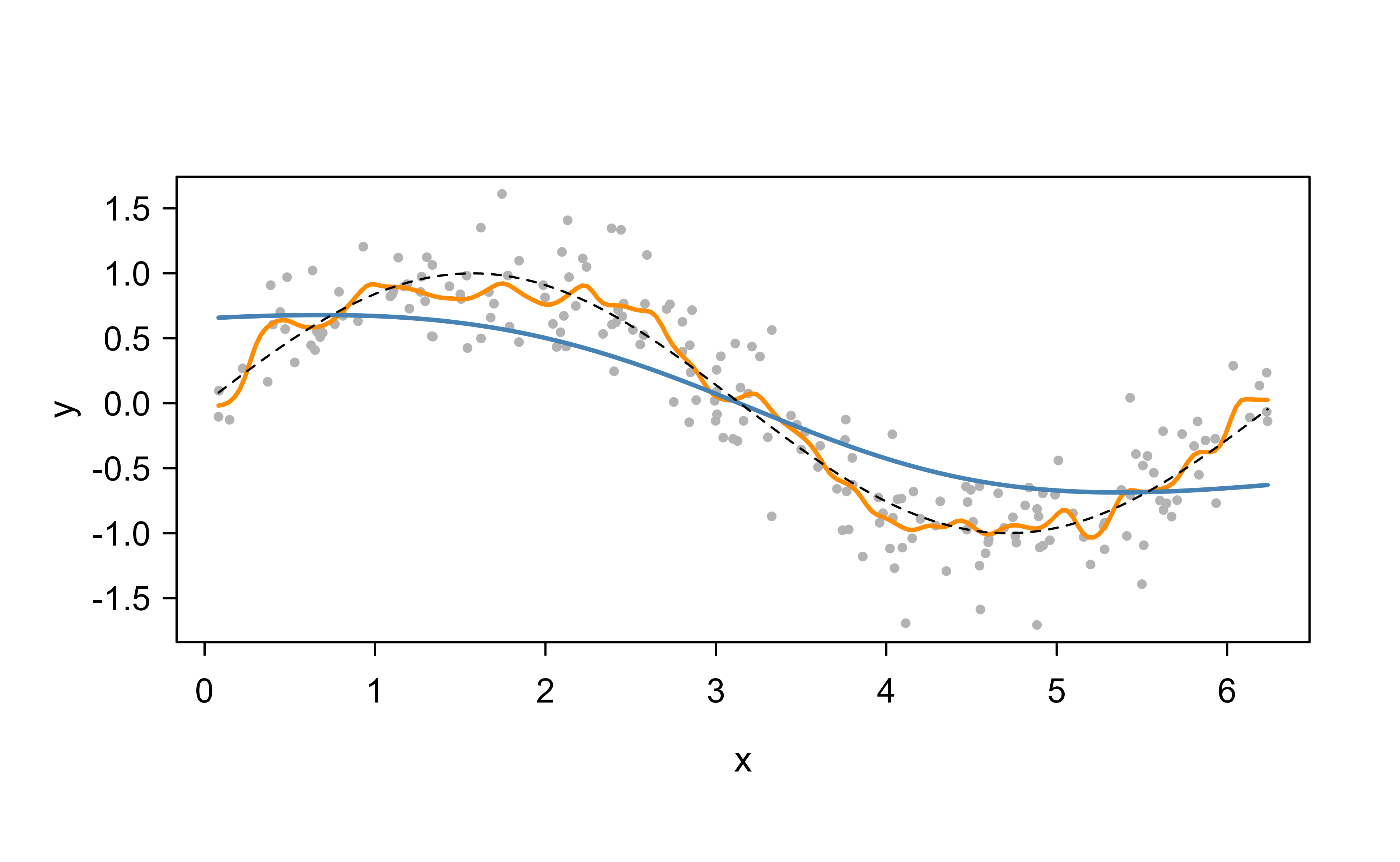
The chapter’s central claim is that the bandwidth $\lambda$ — not the kernel shape — is what controls the bias-variance tradeoff (Section 4.2). That is a claim you can measure. Take a noisy sine wave, where we know the truth, and smooth it with ksmooth (base R’s Nadaraya-Watson estimator) at a tiny and a large bandwidth:

Show code

set.seed(1)
x <- sort(runif(200, 0, 2*pi)); y <- sin(x) + rnorm(200, 0, 0.3)
plot(x, y, col = "grey70", pch = 16, cex = 0.6)
lines(ksmooth(x, y, "normal", bandwidth = 0.2), col = "darkorange", lwd = 2)
lines(ksmooth(x, y, "normal", bandwidth = 3.0), col = "steelblue",  lwd = 2)
curve(sin(x), add = TRUE, lty = 2)   # the truth

Nadaraya-Watson smooths of a noisy sine: a small bandwidth (orange) chases noise; a large one (blue) flattens the signal.

The small-bandwidth fit is jagged (low bias, high variance — it interpolates the noise); the large-bandwidth fit is nearly a flat line (low variance, high bias — it has smoothed the signal away). Neither is right, and the optimum is in between. Because we know the true function here, we can trace the whole tradeoff and find the sweet spot rather than guess it:

Show code

bws <- seq(0.1, 3, by = 0.1)
mse <- sapply(bws, function(b) {
  f <- ksmooth(x, y, "normal", bandwidth = b, x.points = x)
  mean((f$y - sin(f$x))^2, na.rm = TRUE)        # error against the known truth
})
bws[which.min(mse)]                              # the bandwidth that minimizes error
#> [1] 0.6

That single number is the classic U-shaped risk curve in action: error falls as we stop chasing noise, bottoms out, then rises as we start erasing signal. In real problems the truth is unknown, so this minimization is done by cross-validation instead — but the shape of the curve, and the lesson that bandwidth is the dial that matters, are identical.

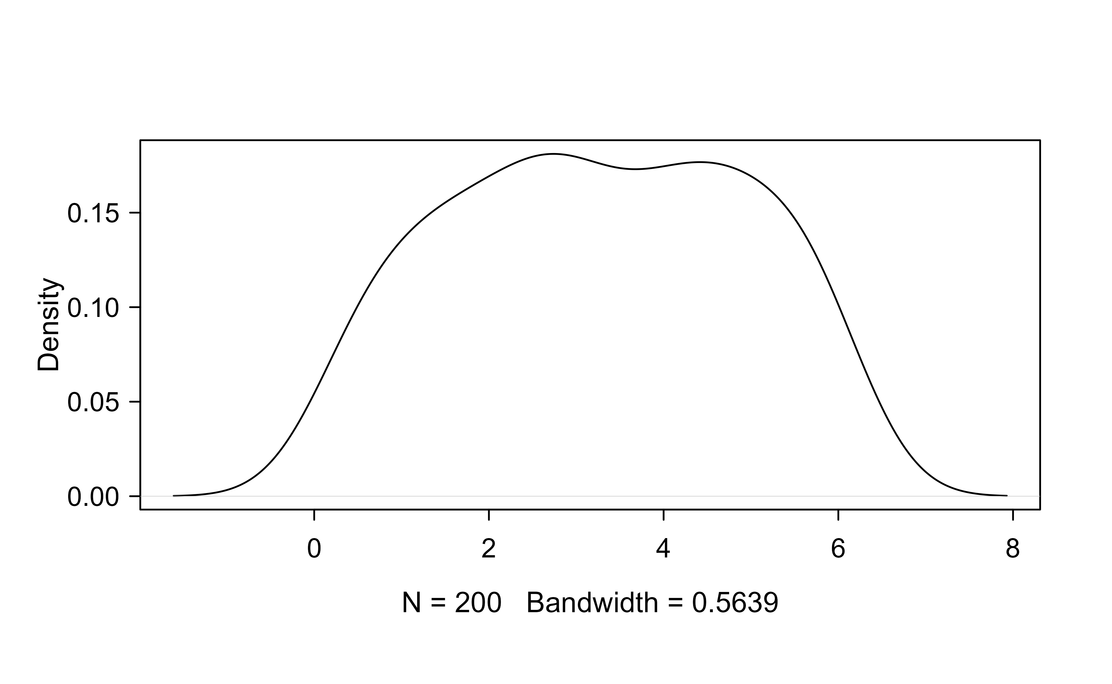
The same kernels estimate densities. Here the bandwidth question becomes “how smooth should the density be,” and R ships principled automatic choices — Silverman’s rule of thumb and the more accurate Sheather-Jones plug-in:

Show code

c(silverman = bw.nrd0(x), sheather_jones = bw.SJ(x))
#>      silverman sheather_jones 
#>      0.5272515      0.5638787
plot(density(x, bw = "SJ"), main = "")

Kernel density estimate of x with a Sheather-Jones bandwidth.

The practical takeaways mirror the theory: pick the kernel for convenience (the Gaussian is the usual default), spend your attention on the bandwidth, prefer a data-driven selector (cross-validation for regression, a plug-in rule for densities) over eyeballing, and remember that estimates near the boundaries are the least trustworthy because the smoothing window there is one-sided.

To recap, this chapter introduced kernels as smooth weighting functions, showed how the Nadaraya-Watson average turns them into a continuous regression estimate, explained how the width $\lambda$ governs the bias-variance tradeoff (and why boundaries are the weak spot), and closed by reusing the same kernels to estimate densities and, through Bayes’ theorem, to classify. For a fuller treatment, see Hastie, Friedman, and Tibshirani (2001) (section 6.6).

Contrast this with ordinary linear regression, which compresses all the training data into a handful of coefficients and then throws the data away. Kernel methods keep everything, which makes prediction more expensive but the model far more flexible.↩︎

# Kernel Smoothing {#sec-kernel} ```{r} #| include: false source("_common.R") ``` Suppose you want to draw a smooth curve through a scatterplot, but you are not willing to commit to a global shape like a straight line or a polynomial. A natural instinct is to look at each point on the x-axis and ask: what is the average response among the observations that sit nearby? Slide that local average across the range of $x$ and you trace out a flexible curve. Kernel smoothing (also called kernel regression) turns this instinct into a precise method. The central idea is to fit a separate but very simple model at each query point $x_0$, using only the observations that are "close" to $x_0$. Closeness is measured by a weighting function, also called a kernel, written $K_\lambda(x_0, x_i)$. The kernel assigns a large weight to observations near $x_0$ and a small (or zero) weight to those far away. Because the weights change smoothly as $x_0$ moves, the resulting estimate $\hat{f}(x)$ is itself smooth across the input space $R^p$. ::: {.callout-tip title="Intuition"} A kernel is just a recipe for "how much should this neighbor count?" Points right next to $x_0$ get a full vote, points a little further away get a fractional vote, and points beyond the kernel's reach get no vote at all. ::: The kernel carries a parameter $\lambda$ that sets the "width" of the neighborhood, that is, how far away an observation can be and still influence the fit. Choosing $\lambda$ is the main modeling decision in kernel smoothing, which is one of its appeals: there is very little to train. The cost shows up at prediction time instead. Kernel smoothers are memory-based methods, meaning the entire training set must be kept around and consulted every time we want a prediction at a new location $x_0$.^[Contrast this with ordinary linear regression, which compresses all the training data into a handful of coefficients and then throws the data away. Kernel methods keep everything, which makes prediction more expensive but the model far more flexible.] In this chapter you will learn how a kernel turns nearby observations into a local estimate, the common choices of kernel and how they differ, how the width $\lambda$ trades bias against variance, and how the same kernel machinery can estimate a probability density rather than a regression function. Kernel smoothing sits between the rigidity of global parametric models and the full flexibility of methods like local regression (@sec-local), which builds directly on the ideas here. ## One-Dimensional Kernel Smoothers To see what a kernel buys us, start from a method you may already know: $k$-nearest neighbors (@sec-knn). The $k$-NN estimate at a point $x$ is simply the average response over the $k$ observations closest to $x$, $$ \hat{f}(x) = Ave (y_i |x_i \in N_k(x)) $$ where $N_k(x)$ refers to the set of $k$ neighbors nearest the point $x$ in squared distance. This works, but it has an awkward feature: as $x$ slides along, observations pop in and out of the neighborhood one at a time, so the fitted curve jumps at each switch. The estimate is a step function, not a smooth one. The fix is to stop treating neighbors as "in or out" and instead weight them continuously by distance. This gives the Nadaraya-Watson kernel-weighted average, $$ \hat{f}(x_0)= \frac{\sum_{i=1}^n K_\lambda(x_0,x_i) y_i}{\sum_{i=1}^n K_\lambda(x_0, x_i)} $$ where the kernel is defined through a function $D$ applied to the scaled distance, $$ K_\lambda(x_0,x) = D(\frac{|x-x_0|}{\lambda}) $$ Read the formula as a weighted average: each $y_i$ is multiplied by its weight $K_\lambda(x_0, x_i)$, and the denominator normalizes the weights so they sum to one. The key difference from nearest neighbors is that the weights now change continuously as $x_0$ moves, rather than in discrete jumps. The result is a smooth curve, which is both more pleasant to look at and, in some settings, more useful to work with. ::: {.callout-important title="Key idea"} Nearest neighbors gives every neighbor an equal vote and everyone else zero. A kernel replaces that hard cutoff with a smooth falloff in influence, and smoothness in the weights produces smoothness in the fit. ::: ### The Nadaraya-Watson estimator as a local average The Nadaraya-Watson estimator is not an arbitrary recipe: it is the solution of a weighted least squares problem, and it is the natural plug-in estimator for the conditional mean. Both views are worth making precise. Assume the data $(x_i, y_i)_{i=1}^n$ are an i.i.d. sample from a joint distribution with density $f_{X,Y}$, and write the regression function as the conditional mean $$ f(x_0) = \mathbb{E}[Y \mid X = x_0] = \int y \, \frac{f_{X,Y}(x_0, y)}{f_X(x_0)} \, dy = \frac{\int y \, f_{X,Y}(x_0, y)\, dy}{f_X(x_0)}. $$ Replace the unknown joint and marginal densities by kernel density estimates. With a kernel $K_\lambda(x_0, x) = \lambda^{-1} D(|x - x_0|/\lambda)$ and a product kernel in $(x, y)$, the estimates are $$ \hat f_X(x_0) = \frac{1}{n}\sum_{i=1}^n K_\lambda(x_0, x_i), \qquad \widehat{f_{X,Y}}(x_0, y) = \frac{1}{n}\sum_{i=1}^n K_\lambda(x_0, x_i)\, K_h(y, y_i). $$ Substituting and using $\int y\, K_h(y, y_i)\, dy = y_i$ (any kernel that is a symmetric density centered at $y_i$ has mean $y_i$, so the bandwidth $h$ cancels) gives $$ \hat f(x_0) = \frac{\frac{1}{n}\sum_i K_\lambda(x_0, x_i)\, y_i}{\frac{1}{n}\sum_i K_\lambda(x_0, x_i)} = \frac{\sum_{i=1}^n K_\lambda(x_0, x_i)\, y_i}{\sum_{i=1}^n K_\lambda(x_0, x_i)}. $$ {#eq-kernel-nw-derivation} This is exactly the Nadaraya-Watson average. The derivation shows the estimator is the conditional mean computed under the kernel density estimate of the data, which is why it inherits both the strengths (consistency) and the weaknesses (boundary bias) of kernel density estimation. Equivalently, $\hat f(x_0)$ is the constant $\beta_0$ that minimizes the locally weighted sum of squares $$ \hat f(x_0) = \arg\min_{\beta_0} \sum_{i=1}^n K_\lambda(x_0, x_i)\,(y_i - \beta_0)^2 . $$ {#eq-kernel-nw-wls} Setting the derivative with respect to $\beta_0$ to zero gives $\sum_i K_\lambda(x_0,x_i)(y_i - \beta_0) = 0$, whose solution is the weighted average in @eq-kernel-nw-derivation. Reading the estimator this way, as fitting a local constant, makes it clear what local regression (@sec-local) changes: it replaces the local constant $\beta_0$ by a local line or polynomial, which is what removes the boundary bias discussed below. ### The estimator is linear in the responses A fact that drives all of the theory is that the fit is linear in $y$. Define the equivalent kernel weights $$ \ell_i(x_0) = \frac{K_\lambda(x_0, x_i)}{\sum_{j=1}^n K_\lambda(x_0, x_j)}, \qquad \hat f(x_0) = \sum_{i=1}^n \ell_i(x_0)\, y_i , $$ {#eq-kernel-linear-smoother} where the weights satisfy $\sum_i \ell_i(x_0) = 1$ for every $x_0$ but in general $\sum_i x_i \,\ell_i(x_0) \neq x_0$. Stacking the fitted values at the training points gives $\hat{\mathbf{y}} = \mathbf{S}\,\mathbf{y}$ with smoother matrix $S_{ij} = \ell_j(x_i)$. Because $\mathbf S$ does not depend on $\mathbf y$, the kernel smoother is a *linear smoother*, exactly like ridge or spline smoothers, and the *effective degrees of freedom* of the fit can be defined as $\mathrm{df}_\lambda = \operatorname{tr}(\mathbf S)$. This single number summarizes complexity across kernels and bandwidths and is what makes different smoothers comparable: a kernel fit with $\operatorname{tr}(\mathbf S) = 8$ is roughly as flexible as a degree-$7$ polynomial regression. ### Choosing the kernel function The shape of $D$ determines how influence falls off with distance. Three choices are standard, and they differ mainly in how abruptly the weight drops to zero and how smooth they are at their edges. The Epanechnikov quadratic kernel is compact, meaning it gives exactly zero weight beyond a finite radius: $$ D(t) = \begin{cases} \frac{3}{4}(1-t^2) & \text{if } |t| \le 1 \\ 0 & \text{otherwise} \end{cases} $$ It is computationally cheap because most observations contribute nothing, but it has no continuous derivative at the boundary of its support, so the fitted curve can show small kinks. The tri-cube kernel is also compact but smoother, with two continuous derivatives at the boundary of its support: $$ D(t) = \begin{cases} (1- |t|^3)^3 & \text{if } |t| \le 1 \\ 0 & \text{otherwise} \end{cases} $$ where $t = |x - x_0|/\lambda$ (the same scaled argument used for every kernel). The extra smoothness at the edges makes it a popular default for local regression. The Gaussian density uses the familiar bell curve as the weighting function: $$ D(t) = \frac{\exp(-\frac{t^2}{2\sigma^2})}{\sqrt{2 \pi}\sigma} $$ where $\sigma$ plays the role of the "width." It is continuously differentiable everywhere, which is attractive, but it has infinite support: every observation gets a nonzero weight, however tiny. That can make it more taxing to compute on large data sets, since no point can be skipped. ::: {.callout-tip} When you need a smooth fit and computation is not a bottleneck, a Gaussian or tri-cube kernel is a safe choice. When the data set is large and you want speed, prefer a compact kernel like the Epanechnikov or tri-cube so that distant points can be ignored entirely. ::: So far $\lambda$ has been a single fixed number, but the neighborhood width need not be constant. With adaptive neighborhoods, the width depends on the location $x_0$, $$ K_\lambda (x_0, x) = D(\frac{|x-x_0|}{h_\lambda(x_0)}) $$ so the kernel can widen in sparse regions and tighten where data are plentiful. A few consequences of these choices are worth keeping in mind: - A large $\lambda$ lowers variance, because we average over more observations (effectively a larger $n$), but it raises bias, because we approximate $f(x_0)$ using observations that lie further from $x_0$. - An adaptive width $h_\lambda(x)$ can hold the bias roughly constant across the input space, but then the variance becomes inversely proportional to the local density of observations: where data are sparse, the estimate is noisier. - The biggest weakness of kernel smoothers is estimation near the boundaries of the data. Near an edge the kernel becomes lopsided, with neighbors on only one side, so the fit is badly biased there. Local regression (@sec-local) was designed partly to correct this boundary bias. ::: {.callout-warning} Trust a kernel smoother least at the left and right ends of the data. The asymmetry of the neighborhood near a boundary systematically pulls the fit toward the interior, and no amount of width tuning fully removes it. ::: ## Selecting the Kernel Width {#sec-kernel-bandwidth} Everything above turns on one number, $\lambda$, the width of the kernel $K_\lambda$. Its precise meaning depends on which kernel you chose: - For the Epanechnikov and tri-cube kernels, $\lambda$ is the radius of the support region, that is, the distance beyond which weights are zero. - For the Gaussian kernel, $\lambda$ is the standard deviation $\sigma$. - For the nearest-neighbor smoother, the role of $\lambda$ is played by $k$, the number of neighbors. In every case the qualitative tradeoff is the same. A smaller width does less averaging, giving higher variance but smaller bias (the fit tracks local wiggles, including noise). A larger width does more averaging, giving lower variance but higher bias (the fit is smoother but can miss real structure). This is the bias-variance tradeoff in its most visible form: $\lambda$ is the dial between an overly jagged fit and an overly flat one. ::: {.callout-tip title="When to use this"} Reach for kernel smoothing when you want a flexible one-dimensional (or low-dimensional) curve, you have enough data to average locally, and you care more about following the data's shape than about an interpretable equation. ::: Because there is no formula that hands you the right width, $\lambda$ is chosen by data-driven tuning, most commonly [Cross-validation]: try a grid of widths, estimate out-of-sample error for each, and keep the width that minimizes it. ### The bias-variance tradeoff, made precise The qualitative statements above can be turned into formulas, and the formulas tell you the optimal bandwidth and the best achievable error rate. Work in one dimension with equally weighted data of size $n$, a kernel that is a symmetric density with $$ \int D(u)\, du = 1, \quad \int u\, D(u)\, du = 0, \quad \mu_2 = \int u^2 D(u)\, du, \quad R(D) = \int D(u)^2\, du, $$ and suppose $f$ is twice continuously differentiable and the design density $g(x)$ is smooth and bounded away from zero near $x_0$. As $n \to \infty$ and $\lambda \to 0$ with $n\lambda \to \infty$, a Taylor expansion of the Nadaraya-Watson estimator gives the standard asymptotic moments at an interior point: $$ \operatorname{Bias}\!\big(\hat f(x_0)\big) \approx \tfrac{1}{2}\lambda^2 \mu_2 \left[ f''(x_0) + \frac{2 f'(x_0) g'(x_0)}{g(x_0)} \right], $$ {#eq-kernel-nw-bias} $$ \operatorname{Var}\!\big(\hat f(x_0)\big) \approx \frac{\sigma^2 R(D)}{n \lambda\, g(x_0)}, $$ {#eq-kernel-nw-var} where $\sigma^2 = \operatorname{Var}(Y \mid X = x_0)$. Two structural facts are visible immediately. First, the bias grows like $\lambda^2$ (wider kernel, more averaging over curvature) while the variance shrinks like $1/(n\lambda)$ (wider kernel averages more points), so the two genuinely pull in opposite directions. Second, the variance is inversely proportional to the local design density $g(x_0)$: where data are sparse the estimate is noisier, which is the formal version of the adaptive-width remark in @sec-kernel. The design-density term $2 f' g'/g$ in @eq-kernel-nw-bias is the *design bias* of the local-constant fit. It does not vanish even where $f$ is linear, and it is exactly the term that local linear regression (@sec-local) annihilates, which is the precise reason local regression is preferred at boundaries and in regions of changing density. Minimizing the asymptotic mean squared error $\operatorname{MSE} = \operatorname{Bias}^2 + \operatorname{Var}$ over $\lambda$ gives the optimal local bandwidth. Writing $b(x_0)$ for the bracketed curvature term in @eq-kernel-nw-bias, $\operatorname{MSE}(\lambda) \approx \tfrac14 \lambda^4 \mu_2^2 b(x_0)^2 + \sigma^2 R(D)/(n\lambda g(x_0))$; differentiating and setting to zero, $$ \lambda_{\text{opt}}(x_0) = \left[ \frac{\sigma^2 R(D)}{\mu_2^2\, b(x_0)^2\, g(x_0)} \right]^{1/5} n^{-1/5}, \qquad \operatorname{MSE}\big(\lambda_{\text{opt}}\big) = O\!\left(n^{-4/5}\right). $$ {#eq-kernel-opt-bandwidth} This is the canonical rate for one-dimensional nonparametric smoothing: the best bandwidth shrinks like $n^{-1/5}$ and the pointwise error converges at $n^{-4/5}$, strictly slower than the $n^{-1}$ MSE of a correctly specified parametric model. That gap is the price of not committing to a global form, and it cannot be beaten without extra smoothness assumptions on $f$. ::: {.callout-note title="Curse of dimensionality"} In $p$ dimensions with a product kernel the same expansion gives bias $O(\lambda^2)$ and variance $O\!\big(1/(n\lambda^p)\big)$, so the optimal bandwidth is $\lambda_{\text{opt}} \propto n^{-1/(p+4)}$ and the optimal MSE is $O\!\big(n^{-4/(p+4)}\big)$. The rate degrades sharply with $p$: matching the accuracy a one-dimensional smoother reaches with $n$ points requires roughly $n^{(p+4)/5}$ points in $p$ dimensions. This is why raw kernel smoothing is a low-dimensional tool, and why high-dimensional problems call for structure such as additivity (@sec-gam) or projection. ::: ### Practical bandwidth selection In practice three routes to a bandwidth are common, in increasing order of robustness. *Leave-one-out cross-validation, computed cheaply.* Because the smoother is linear (@eq-kernel-linear-smoother), the leave-one-out residual has a closed form that avoids refitting $n$ times. If $S_{ii}$ is the $i$th diagonal of the smoother matrix, then $$ y_i - \hat f^{(-i)}(x_i) = \frac{y_i - \hat f(x_i)}{1 - S_{ii}}, \qquad \operatorname{CV}(\lambda) = \frac{1}{n}\sum_{i=1}^n \left( \frac{y_i - \hat f(x_i)}{1 - S_{ii}} \right)^2 , $$ {#eq-kernel-loocv} so a full LOOCV curve costs one fit per candidate $\lambda$, not $n$. The same identity underlies generalized cross-validation, which replaces $S_{ii}$ by the average $\operatorname{tr}(\mathbf S)/n$. *Plug-in rules.* @eq-kernel-opt-bandwidth depends only on $\sigma^2$, the design density, and the curvature functional $\int b(x)^2 g(x)\, dx$. Plug-in methods estimate these from a pilot fit and substitute them, giving a bandwidth without a search. They converge faster than cross-validation but require the smoothness assumptions to hold. *Rules of thumb (density estimation).* For Gaussian KDE of a roughly Gaussian sample, Silverman's rule sets $\lambda = 0.9\, \min(\hat\sigma, \widehat{\mathrm{IQR}}/1.34)\, n^{-1/5}$, which minimizes asymptotic integrated squared error under normality and is the default in `density()`. It oversmooths multimodal densities, so treat it as a starting point and reduce $\lambda$ if structure is suspected. The leave-one-out shortcut in @eq-kernel-loocv is worth checking directly: the closed-form residual should equal an honest refit that deletes each point. The following base R simulation confirms it for a Gaussian Nadaraya-Watson smoother. ```{r} #| label: loocv-identity-check set.seed(1) n <- 40 x <- sort(runif(n)); y <- sin(2 * pi * x) + rnorm(n, sd = 0.2) lambda <- 0.1 # Smoother matrix S with row-normalized Gaussian weights W <- outer(x, x, function(a, b) dnorm((a - b) / lambda)) S <- W / rowSums(W) fit <- as.vector(S %*% y) # Closed-form LOO residuals via the diagonal of S loo_closed <- (y - fit) / (1 - diag(S)) # Brute-force LOO: delete each point and refit loo_brute <- sapply(seq_len(n), function(i) { w <- dnorm((x[i] - x[-i]) / lambda) y[i] - sum(w * y[-i]) / sum(w) }) max(abs(loo_closed - loo_brute)) # ~ 0 up to floating point ``` A useful diagnostic across all routes: plot the fit at several bandwidths spanning the cross-validation minimum. A good $\lambda$ sits in a region where the fit is visually stable; if the curve changes character drastically for small changes in $\lambda$, the data do not pin the bandwidth down and the smoothest defensible choice should be preferred. ::: {.callout-warning title="Failure modes"} Kernel smoothers break in predictable ways: (i) at boundaries, where the one-sided neighborhood induces $O(\lambda)$ bias rather than $O(\lambda^2)$, fixed only by local polynomials; (ii) under heteroscedastic or heavy-tailed noise, where the local average is not robust and a single outlier drags the fit; (iii) in regions of sharply varying density, where a global bandwidth is simultaneously too wide where data are dense and too narrow where data are sparse; and (iv) in moderate to high dimension, where the curse of dimensionality empties every neighborhood. ::: ## Kernel Density Estimation Kernels did not begin as a regression tool. Their original job was to estimate a probability density, and that use is still common today. The shift in goal is small: instead of averaging response values $y_i$ near $x_0$, we count how many observations pile up near $x_0$, which tells us how probable that region is. Suppose we have a random sample $x_1, \dots, x_n$ drawn from an unknown probability density $f_X(x)$, and we want to estimate $f_X$ at a point $x_0$, working in one dimension so $X \in R$. The Parzen estimate places a small kernel bump at every observation and adds them up: $$ \hat{f}_X(x_0) = \frac{1}{n \lambda}\sum_{i=1}^n K_\lambda (x_0, x_i) $$ A common choice is the Gaussian kernel with standard deviation $\lambda$. The leading factor $\frac{1}{n\lambda}$ normalizes the result so that it integrates to one, as a density must. The same construction extends to higher dimensions by replacing the one-dimensional kernel with a multivariate (Gaussian) kernel. ::: {.callout-tip title="Intuition"} Picture dropping a tiny mound of sand on the number line at each data point. Where points cluster, the mounds overlap and pile high; where points are scarce, the sand is thin. The resulting profile, rescaled to integrate to one, is the estimated density. ::: ### Bias, variance, and the optimal density bandwidth The same expansion that governed regression applies to the density estimate, and here it is cleaner because there is no design density to contend with. Write the estimator with a kernel $D$ that is a symmetric density as $\hat f_X(x_0) = \tfrac{1}{n\lambda}\sum_i D\!\big((x_0 - x_i)/\lambda\big)$. Taking the expectation over one observation, $$ \mathbb{E}\,\hat f_X(x_0) = \frac{1}{\lambda}\int D\!\Big(\frac{x_0 - u}{\lambda}\Big) f_X(u)\, du = \int D(t)\, f_X(x_0 - \lambda t)\, dt , $$ and a second-order Taylor expansion $f_X(x_0 - \lambda t) = f_X(x_0) - \lambda t f_X'(x_0) + \tfrac12 \lambda^2 t^2 f_X''(x_0) + o(\lambda^2)$, together with $\int D = 1$ and $\int t D(t)\, dt = 0$, yields $$ \operatorname{Bias}\!\big(\hat f_X(x_0)\big) \approx \tfrac{1}{2}\lambda^2 \mu_2\, f_X''(x_0), \qquad \operatorname{Var}\!\big(\hat f_X(x_0)\big) \approx \frac{f_X(x_0)\, R(D)}{n\lambda} . $$ {#eq-kernel-kde-bias-var} The bias is proportional to the curvature $f_X''$: a Gaussian KDE flattens peaks and fills valleys, the same oversmoothing that Silverman's rule risks. Integrating the mean squared error over $x_0$ gives the asymptotic mean integrated squared error, $$ \operatorname{AMISE}(\lambda) = \frac{R(D)}{n\lambda} + \frac{1}{4}\lambda^4 \mu_2^2 \int f_X''(x)^2\, dx , $$ and minimizing over $\lambda$ gives the optimal density bandwidth and rate, $$ \lambda_{\text{opt}} = \left[ \frac{R(D)}{\mu_2^2 \int (f_X'')^2}\right]^{1/5} n^{-1/5}, \qquad \operatorname{AMISE}\big(\lambda_{\text{opt}}\big) = O\!\left(n^{-4/5}\right). $$ {#eq-kernel-kde-amise} The $n^{-1/5}$ bandwidth and $n^{-4/5}$ error mirror the regression case, and substituting the standard normal for $f_X$ and the Gaussian for $D$ in @eq-kernel-kde-amise reproduces Silverman's rule exactly. Density estimates are not only descriptive: they plug directly into classification through Bayes' theorem. Suppose there are $J$ classes, and we fit a separate nonparametric density $\hat{f}_j (X)$ for $j = 1, \dots, J$, one per class. Given a prior probability $\hat{\pi}_j$ for each class (these might come from the observed class proportions or from outside knowledge), the posterior probability that a new point $x_0$ belongs to class $j$ is $$ \hat{P}(G=j | X=x_0) = \frac{\hat{\pi}_j \hat{f}_j (x_0)}{\sum_{k=1}^J \hat{\pi}_k \hat{f}_k (x_0)} $$ In words, we weight each class density by its prior and renormalize across classes, then assign $x_0$ to whichever class comes out largest. This is the kernel-based cousin of methods like the naive Bayes (@sec-naive-bayes) and discriminant (@sec-discriminant-analysis) classifiers. ## Kernel Smoothing in R: A Worked Example {#sec-kernel-worked} The chapter's central claim is that the bandwidth $\lambda$ --- not the kernel shape --- is what controls the bias-variance tradeoff (@sec-kernel-bandwidth). That is a claim you can measure. Take a noisy sine wave, where we know the truth, and smooth it with `ksmooth` (base R's Nadaraya-Watson estimator) at a tiny and a large bandwidth: ```{r} #| label: kernel-data #| fig-cap: "Nadaraya-Watson smooths of a noisy sine: a small bandwidth (orange) chases noise; a large one (blue) flattens the signal." set.seed(1) x <- sort(runif(200, 0, 2*pi)); y <- sin(x) + rnorm(200, 0, 0.3) plot(x, y, col = "grey70", pch = 16, cex = 0.6) lines(ksmooth(x, y, "normal", bandwidth = 0.2), col = "darkorange", lwd = 2) lines(ksmooth(x, y, "normal", bandwidth = 3.0), col = "steelblue", lwd = 2) curve(sin(x), add = TRUE, lty = 2) # the truth ``` The small-bandwidth fit is jagged (low bias, high variance --- it interpolates the noise); the large-bandwidth fit is nearly a flat line (low variance, high bias --- it has smoothed the signal away). Neither is right, and the optimum is in between. Because we know the true function here, we can trace the whole tradeoff and find the sweet spot rather than guess it: ```{r} #| label: kernel-ucurve bws <- seq(0.1, 3, by = 0.1) mse <- sapply(bws, function(b) { f <- ksmooth(x, y, "normal", bandwidth = b, x.points = x) mean((f$y - sin(f$x))^2, na.rm = TRUE) # error against the known truth }) bws[which.min(mse)] # the bandwidth that minimizes error ``` That single number is the classic U-shaped risk curve in action: error falls as we stop chasing noise, bottoms out, then rises as we start erasing signal. In real problems the truth is unknown, so this minimization is done by cross-validation instead --- but the shape of the curve, and the lesson that bandwidth is the dial that matters, are identical. The same kernels estimate densities. Here the bandwidth question becomes "how smooth should the density be," and R ships principled automatic choices --- Silverman's rule of thumb and the more accurate Sheather-Jones plug-in: ```{r} #| label: kernel-kde #| fig-cap: "Kernel density estimate of x with a Sheather-Jones bandwidth." c(silverman = bw.nrd0(x), sheather_jones = bw.SJ(x)) plot(density(x, bw = "SJ"), main = "") ``` The practical takeaways mirror the theory: pick the kernel for convenience (the Gaussian is the usual default), spend your attention on the bandwidth, prefer a data-driven selector (cross-validation for regression, a plug-in rule for densities) over eyeballing, and remember that estimates near the boundaries are the least trustworthy because the smoothing window there is one-sided. To recap, this chapter introduced kernels as smooth weighting functions, showed how the Nadaraya-Watson average turns them into a continuous regression estimate, explained how the width $\lambda$ governs the bias-variance tradeoff (and why boundaries are the weak spot), and closed by reusing the same kernels to estimate densities and, through Bayes' theorem, to classify. For a fuller treatment, see @hastie2001a (section 6.6).