65  Multi-Armed Bandits

Picture a row of slot machines in a casino. Each machine pays out at its own unknown rate, and you have a fixed number of coins to spend. Every pull of a lever (an “arm”) gives you a payout drawn from that machine’s hidden distribution, and nothing else. You do not get to see what the other machines would have paid on that same turn. Your goal is to walk away with as much money as possible. The catch is that the only way to learn which machine is best is to spend coins finding out, and every coin spent learning is a coin you did not spend on the machine you already suspect is best.

This is the multi-armed bandit problem, and it is the cleanest setting in which to study a tension that runs through all of sequential decision making: the pull between exploration (gathering information about arms you are unsure of) and exploitation (cashing in on the arm that currently looks best). The name comes from the slang “one-armed bandit” for a slot machine; a bank of them is a multi-armed bandit.¹

The reason this toy problem matters is that the same structure appears everywhere a system makes repeated choices and learns only from the choice it made. Which of five ad creatives to show. Which headline to put on an article. Which dosage to try next in an adaptive experiment. In each case you commit to one option, observe a noisy reward, and never see the counterfactual. By the end of this chapter you will understand how to measure how well an algorithm handles this, and you will have three concrete strategies, epsilon-greedy, Upper Confidence Bound, and Thompson sampling, with a runnable simulation that pits them against each other.

Intuition

If you always exploit, you may lock onto an arm that looked good early by luck and never discover the truly best one. If you always explore, you waste pulls on arms you already know are bad. Good bandit algorithms explore aggressively when they are uncertain and taper off as evidence accumulates.

This chapter treats the stochastic, context-free bandit: the arms’ reward distributions are fixed and do not depend on any side information. When each round comes with features that should shape the choice, you have a contextual bandit, covered in the contextual bandits chapter (Chapter 72). The methods here are the building blocks that the contextual version generalizes.

65.1 The stochastic k-armed bandit

We have \(k\) arms, indexed \(a \in \{1, 2, \dots, k\}\). Each arm \(a\) has a fixed but unknown reward distribution with mean \[ q_*(a) = \mathbb{E}[R \mid A = a], \] where \(A\) is the arm we choose and \(R\) is the reward we receive. The quantity \(q_*(a)\) is called the action value of arm \(a\): it is the average reward you would get if you pulled that arm forever.

At each time step \(t = 1, 2, \dots, T\) we select an arm \(A_t\) and observe a reward \(R_t\) drawn independently from the distribution of arm \(A_t\). The number \(T\) is the horizon. Because we only ever see the reward of the arm we pulled, we must estimate the action values from data. The natural estimate is the sample mean of rewards observed from arm \(a\) up to time \(t\): \[ Q_t(a) = \frac{\sum_{s=1}^{t-1} R_s \,\mathbb{1}[A_s = a]}{\sum_{s=1}^{t-1} \mathbb{1}[A_s = a]}, \] where \(\mathbb{1}[\cdot]\) is the indicator function. Write \(N_t(a) = \sum_{s=1}^{t-1} \mathbb{1}[A_s = a]\) for the number of times arm \(a\) has been pulled before time \(t\). As \(N_t(a)\) grows, \(Q_t(a)\) converges to \(q_*(a)\) by the law of large numbers.

A convenient fact: the sample mean can be updated online without storing every reward. If \(Q_n\) is the average of the first \(n\) rewards from an arm and a new reward \(R_{n+1}\) arrives, \[ Q_{n+1} = Q_n + \frac{1}{n+1}\bigl(R_{n+1} - Q_n\bigr). \] This “old estimate plus a step toward the new observation” form is the same shape as the update rules used throughout reinforcement learning.

To see that this is exact and not an approximation, start from the definition \(Q_{n+1} = \frac{1}{n+1}\sum_{i=1}^{n+1} R_i\) and peel off the last term: \[ Q_{n+1} = \frac{1}{n+1}\left( R_{n+1} + \sum_{i=1}^{n} R_i \right) = \frac{1}{n+1}\bigl( R_{n+1} + n Q_n \bigr) = Q_n + \frac{1}{n+1}\bigl( R_{n+1} - Q_n \bigr). \tag{65.1}\] The general template \(Q \leftarrow Q + \alpha_n (R - Q)\) with step size \(\alpha_n = 1/(n+1)\) recovers the sample mean. Two facts about the step-size schedule are worth stating, because they govern whether the estimate converges. The Robbins-Monro conditions \(\sum_n \alpha_n = \infty\) and \(\sum_n \alpha_n^2 < \infty\) guarantee almost-sure convergence of the stochastic average to \(q_*(a)\); the harmonic schedule \(\alpha_n = 1/n\) satisfies both (\(\sum 1/n = \infty\), \(\sum 1/n^2 < \infty\)). A constant step size \(\alpha_n = \beta\) violates the second condition, so it does not converge to a point; instead it produces an exponentially weighted moving average that keeps tracking a changing target, which is exactly why it is preferred in the nonstationary case discussed later. Unrolling the constant-\(\beta\) recursion makes the weighting explicit: \[ Q_{n} = (1-\beta)^{n} Q_0 + \sum_{i=1}^{n} \beta (1-\beta)^{\,n-i} R_i, \tag{65.2}\] so the weight on a reward decays geometrically with its age and the influence of the initial guess \(Q_0\) vanishes geometrically.

Note

We will run our demos with Bernoulli arms, where each reward is \(0\) or \(1\) and \(q_*(a)\) is simply the probability that arm \(a\) returns a \(1\). This is the model for click-through rates, conversion rates, and any success/failure outcome. The estimate \(Q_t(a)\) is then just the observed success rate of arm \(a\).

65.2 Regret: how we keep score

We need a yardstick. The obvious one, total reward collected, is hard to read because it depends on the unknown arm values. Instead we measure how much worse we did than an oracle that knew the best arm from the start. Let \[ q_* = \max_a q_*(a) \] be the value of the best arm. The expected cumulative regret after \(T\) rounds is \[ \mathcal{R}(T) = \sum_{t=1}^{T} \bigl(q_* - \mathbb{E}[q_*(A_t)]\bigr) = T q_* - \sum_{t=1}^{T} \mathbb{E}[q_*(A_t)]. \] Regret is the total reward we gave up by not always playing the best arm. It can never be negative, and an algorithm that found and stuck to the best arm immediately would have regret zero. Lower is better.

It is often cleaner to write regret in terms of the gaps \(\Delta_a = q_* - q_*(a)\), the shortfall of arm \(a\) relative to the best. If \(N_T(a)\) is the number of times arm \(a\) was pulled over the whole run, then \[ \mathcal{R}(T) = \sum_{a} \Delta_a \, \mathbb{E}[N_T(a)]. \] This decomposition says something important: regret comes entirely from pulling suboptimal arms, weighted by how bad each one is. To keep regret low you must pull a poor arm only a small number of times, and the worse it is (large \(\Delta_a\)), the fewer pulls you can afford.

Key idea

A good algorithm has regret that grows sublinearly in \(T\), meaning \(\mathcal{R}(T)/T \to 0\). Linear regret means a fixed fraction of every round is wasted forever, which is what happens if you keep exploring at a constant rate. Sublinear regret means the per-round penalty shrinks as you learn.

Lai and Robbins (1985) proved that no algorithm can beat regret of order \(\log T\) for this problem: any reasonable strategy must pull each suboptimal arm at least about \(\log T\) times to be statistically sure it is suboptimal. The good algorithms below achieve this logarithmic rate; the naive one does not.

65.2.1 The Lai-Robbins lower bound, precisely

The informal statement above can be made exact, and the exact form tells you what quantity actually controls the difficulty of the problem. Restrict attention to policies that are consistent, meaning the regret is sub-polynomial, \(\mathcal{R}(T) = o(T^{\gamma})\) for every \(\gamma > 0\), on every problem instance in a given parametric family. (Consistency rules out cheating policies that hard-code one arm and do brilliantly on instances where that arm happens to be best while doing terribly elsewhere.) For any such policy, Lai and Robbins showed that for each suboptimal arm \(a\), \[ \liminf_{T \to \infty} \frac{\mathbb{E}[N_T(a)]}{\log T} \ge \frac{1}{D_{\mathrm{KL}}\!\bigl(P_a \,\|\, P_{a^*}\bigr)}, \tag{65.3}\] where \(P_a\) is the reward distribution of arm \(a\), \(P_{a^*}\) is that of the optimal arm, and \(D_{\mathrm{KL}}(P\|Q) = \int \log \tfrac{dP}{dQ}\, dP\) is the Kullback-Leibler divergence. Substituting into the gap decomposition \(\mathcal{R}(T) = \sum_a \Delta_a\, \mathbb{E}[N_T(a)]\) gives the regret lower bound \[ \liminf_{T\to\infty} \frac{\mathcal{R}(T)}{\log T} \ge \sum_{a : \Delta_a > 0} \frac{\Delta_a}{D_{\mathrm{KL}}\!\bigl(P_a \,\|\, P_{a^*}\bigr)}. \tag{65.4}\]

The intuition behind the proof is a change-of-measure (or hypothesis-testing) argument. To be consistent the policy must, on the true instance, almost never pull arm \(a\). But consider an alternative instance, identical except that arm \(a\)’s mean is nudged just above \(q_*\) so that \(a\) becomes optimal. A consistent policy must pull \(a\) often on that alternative. The only way to behave so differently on two instances that differ only in arm \(a\)’s reward distribution is to have collected enough samples from \(a\) to statistically distinguish \(P_a\) from the nudged distribution. The number of samples needed to tell two distributions apart with high confidence scales like \(\log T\) divided by their KL divergence, by the same information-theoretic accounting that underlies the Neyman-Pearson lemma and Stein’s lemma. That is the source of both the \(\log T\) and the \(1/D_{\mathrm{KL}}\).

Note

For Bernoulli arms with means \(p\) and \(q\) the relevant divergence is \(D_{\mathrm{KL}}(p\|q) = p\log\frac{p}{q} + (1-p)\log\frac{1-p}{1-q}\), and Pinsker’s inequality gives \(D_{\mathrm{KL}}(p\|q) \ge 2(p-q)^2 = 2\Delta_a^2\). Plugging this into Equation 65.4 turns the sharp KL bound into the looser but more readable gap-based form \(\mathcal{R}(T) \gtrsim \sum_a \frac{1}{2\Delta_a}\log T\). The KL form is tight; the gap form is what most upper bounds are stated against, which is why UCB and Thompson sampling match the lower bound up to constants rather than exactly.

65.3 Epsilon-greedy

The simplest workable strategy is epsilon-greedy. Fix a small probability \(\varepsilon \in (0, 1)\). At each step, with probability \(1 - \varepsilon\) pull the arm with the highest current estimate (exploit), and with probability \(\varepsilon\) pull an arm chosen uniformly at random (explore): \[ A_t = \begin{cases} \arg\max_a Q_t(a) & \text{with probability } 1 - \varepsilon, \\ \text{uniform random arm} & \text{with probability } \varepsilon. \end{cases} \]

The appeal is that it is trivial to implement and it never stops exploring, so it cannot get permanently stuck on a wrong arm. The drawback follows from the same fact: with a fixed \(\varepsilon\), the algorithm wastes a fraction \(\varepsilon\) of its pulls on random arms forever, even long after it has identified the best one. That gives regret of order \(\varepsilon T\), which is linear. You pay a constant tax per round.

The linear rate is not just a hand-wave; it follows from the per-round regret. On any round, with probability \(\varepsilon\) the algorithm explores uniformly, so even granting that it always exploits the truly best arm (the most favorable possible assumption once estimates have converged), its expected instantaneous regret is at least the regret of a uniform random pull scaled by \(\varepsilon\): \[ q_* - \mathbb{E}[q_*(A_t)] \;\ge\; \varepsilon \cdot \frac{1}{k}\sum_{a} \Delta_a \;=\; \varepsilon\, \bar\Delta, \qquad \bar\Delta = \frac{1}{k}\sum_a \Delta_a . \] Summing over \(t = 1, \dots, T\) gives \(\mathcal{R}(T) \ge \varepsilon\, \bar\Delta\, T\), a regret that grows linearly with the horizon no matter how good the exploitation becomes. The constant tax is exactly \(\varepsilon \bar\Delta\) per round.

65.3.1 Recovering the logarithmic rate with a decaying schedule

The cure is to let \(\varepsilon\) shrink at the right speed. The schedule must explore each suboptimal arm enough to identify it (which needs order \(\log t\) exploratory pulls per arm) while spending an ever-smaller share of rounds doing so. Auer, Cesa-Bianchi, and Fischer (2002) showed that the schedule \[ \varepsilon_t = \min\!\left\{ 1, \; \frac{c\,k}{d^2\, t} \right\}, \qquad 0 < d \le \min_{a:\Delta_a>0}\Delta_a, \tag{65.5}\] with a suitable constant \(c > 0\), achieves instantaneous regret of order \(1/t\) and therefore cumulative regret of order \(\sum_{t} 1/t = O(\log T)\), matching the Lai-Robbins rate up to constants. The mechanism is a balance of two competing error sources. The expected number of exploratory pulls of any arm up to time \(T\) is \(\sum_{t \le T} \varepsilon_t / k \approx (c/d^2)\log T\), which contributes \(O(\log T)\) regret directly. Against this, the probability that the greedy step picks a wrong arm because its sample mean is inflated decays fast enough (by a Hoeffding bound, since after \(\Theta(\log t)\) pulls the estimate concentrates within \(d/2\) of the truth with probability \(1 - O(1/t)\)) that the exploitation error also sums to \(O(\log T)\). The two pieces are balanced precisely when \(\varepsilon_t \propto 1/t\), which is the schedule above.

Warning

The decaying schedule in Equation 65.5 needs a lower bound \(d\) on the smallest gap to set its constant. Choosing \(d\) too large under-explores and risks locking onto a wrong arm; too small over-explores and inflates the constant. This gap-dependence is the price epsilon-greedy pays for its simplicity, and it is exactly the kind of problem-specific tuning that UCB and Thompson sampling avoid by adapting their exploration to the observed data.

Warning

A fixed \(\varepsilon\) guarantees linear regret. To recover the logarithmic rate you must let \(\varepsilon\) decay over time, for example \(\varepsilon_t \propto 1/t\). In practice a small constant such as \(\varepsilon = 0.1\) is a common, reasonable default when the horizon is short or when you expect arm values to drift, because it keeps a steady trickle of exploration.

A second weakness of epsilon-greedy is that its exploration is undirected: when it explores, it picks uniformly among all arms, including ones it already knows are terrible. It does not focus its exploration on the arms it is most uncertain about. The next two methods fix exactly this.

65.4 Optimistic initialization

Before adding more machinery, there is a cheap trick worth knowing. Optimistic initialization seeds every arm’s estimate with a value higher than any plausible true value, for Bernoulli arms you might set \(Q_1(a) = 1\) for all \(a\). Then run a purely greedy policy (no random exploration). Because every untried arm looks fantastic, the greedy rule is forced to try each arm at least once, and each disappointing reward pulls that arm’s estimate down toward reality. Exploration happens automatically as a side effect of optimism, then fades as the estimates settle.

Intuition

Optimism in the face of uncertainty: assume an arm is great until it proves otherwise. This single idea, “act as if the unknown is good,” is the seed of the UCB algorithm below, which makes the optimism precise and time-aware rather than a one-time initialization.

The limitation is that optimistic initialization only drives early exploration. Once the inflated initial values wash out, the policy is greedy and will not revisit a discarded arm, so it is fragile if rewards are nonstationary. It is best seen as a complement to other ideas rather than a standalone solution.

65.5 Upper Confidence Bound (UCB1)

The trouble with greedy methods is that they trust their point estimate \(Q_t(a)\) and ignore how uncertain it is. An arm pulled twice with estimate \(0.5\) and an arm pulled two hundred times with estimate \(0.5\) are very different situations: the first might really be excellent and we just have not seen it yet. Upper Confidence Bound methods act on the optimistic edge of what is plausible, not the center.

The reasoning rests on a concentration inequality. Hoeffding’s inequality says that for independent rewards bounded in \([0,1]\) with sample mean \(Q_t(a)\) over \(N_t(a)\) pulls, \[ \Pr\bigl(q_*(a) > Q_t(a) + u\bigr) \le e^{-2 N_t(a) u^2}. \] This bounds the chance that the true value exceeds our estimate by more than \(u\). If we want this failure probability to shrink like \(t^{-4}\) (a schedule that turns out to give the right exploration rate), we set \(e^{-2 N_t(a) u^2} = t^{-4}\) and solve for the confidence width \(u\): \[ -2 N_t(a) u^2 = -4 \log t \quad\Longrightarrow\quad u = \sqrt{\frac{2 \log t}{N_t(a)}}. \] The UCB1 algorithm of Auer, Cesa-Bianchi, and Fischer (2002) then pulls the arm with the largest optimistic value, the estimate plus this width: \[ A_t = \arg\max_a \left[ Q_t(a) + c \sqrt{\frac{\log t}{N_t(a)}} \right], \] with the constant \(c = \sqrt{2}\) recovering the derivation above (any \(c > 0\) is a valid tuning knob).

Read the formula as two competing terms. The first, \(Q_t(a)\), is the exploitation term: it favors arms that have paid well. The second, the square-root exploration bonus, is large when \(N_t(a)\) is small (we have barely tried this arm) and shrinks as we pull it more; the \(\log t\) in the numerator slowly revives the bonus over time so that a long-neglected arm eventually gets reconsidered. An arm is selected either because it looks good or because we are unsure about it, and the bonus quantifies exactly how unsure.

Key idea

UCB needs no random coin flips. Its exploration is directed: the bonus channels pulls toward arms whose value is genuinely uncertain, not uniformly across all arms. This is why UCB achieves regret of order \(\log T\), matching the Lai-Robbins lower bound, while fixed epsilon-greedy does not.

A practical detail: the bonus is infinite when \(N_t(a) = 0\), so UCB1 begins by pulling each arm once to initialize. After that the formula takes over.

65.5.1 Why the \(t^{-4}\) schedule, and the role of the union bound

The choice to drive the per-arm failure probability to \(t^{-4}\) rather than, say, \(t^{-2}\) deserves justification, because it is not arbitrary. Two confidence events must hold simultaneously for UCB to make a sound decision on round \(t\): the optimal arm’s index must not underestimate its value (so the optimal arm is not unfairly passed over), and a suboptimal arm’s index must not overestimate its value by too much. Each is a one-sided Hoeffding event. But \(N_t(a)\) is itself random, so to apply the fixed-sample Hoeffding bound we union over all possible values of the count, \(N_t(a) \in \{1, \dots, t\}\), and over both arms involved. A bound of \(t^{-4}\) on each event, summed over the at most \(2t\) relevant (count, arm) pairs, yields a total failure probability of order \(2t \cdot t^{-4} = 2 t^{-3}\) on round \(t\), and \(\sum_t 2 t^{-3} < \infty\). A weaker per-event bound such as \(t^{-2}\) would leave \(\sum_t 2t \cdot t^{-2} = \sum_t 2/t\), which diverges, and the accumulated failure mass would itself contribute linear regret. The exponent \(4\) is the smallest clean integer that makes the doubly-summed bad-event probability finite, which is why it appears in the width derivation above.

65.5.2 Regret upper bound for UCB1

We can now show that UCB1 attains the logarithmic rate, and the proof reveals exactly how many times each bad arm gets pulled. Fix a suboptimal arm \(a\) with gap \(\Delta_a > 0\). The claim is that once \(a\) has been pulled \[ N_t(a) \ge \ell_a := \left\lceil \frac{8 \log T}{\Delta_a^2} \right\rceil \] times, its exploration bonus has shrunk enough that, on the high-probability event where all confidence intervals hold, its upper confidence index falls below that of the optimal arm and it is no longer selected. To see this, suppose UCB picks \(a\) over the optimal arm \(a^*\) at round \(t\). By the selection rule its index is the largest, so in particular \[ Q_t(a) + \sqrt{\frac{2\log t}{N_t(a)}} \;\ge\; Q_t(a^*) + \sqrt{\frac{2\log t}{N_t(a^*)}}. \] On the good event the right side is at least \(q_*\) (the optimal index does not underestimate), and the left side is at most \(q_*(a) + 2\sqrt{2\log t / N_t(a)}\) (the empirical mean of \(a\) does not exceed its true mean by more than one confidence width). Chaining these, \[ q_* \;\le\; q_*(a) + 2\sqrt{\frac{2\log t}{N_t(a)}} \quad\Longrightarrow\quad \Delta_a \le 2\sqrt{\frac{2\log t}{N_t(a)}} \quad\Longrightarrow\quad N_t(a) \le \frac{8\log t}{\Delta_a^2} \le \frac{8\log T}{\Delta_a^2}. \tag{65.6}\] So on the good event a suboptimal arm cannot be chosen once its count exceeds \(8\log T / \Delta_a^2\). Adding the bounded contribution from the rare bad events (the union-bound tail above, which sums to a constant of order \(\sum_t t^{-3}\), contributing a \(1 + \pi^2/3\) additive term per arm), the expected number of pulls satisfies \[ \mathbb{E}[N_T(a)] \;\le\; \frac{8\log T}{\Delta_a^2} + 1 + \frac{\pi^2}{3}. \tag{65.7}\] Substituting into the gap decomposition \(\mathcal{R}(T) = \sum_a \Delta_a \mathbb{E}[N_T(a)]\) gives the instance-dependent bound \[ \mathcal{R}(T) \;\le\; \sum_{a : \Delta_a > 0} \left( \frac{8\log T}{\Delta_a} + \Bigl(1 + \tfrac{\pi^2}{3}\Bigr)\Delta_a \right) \;=\; O\!\left(\sum_{a:\Delta_a>0}\frac{\log T}{\Delta_a}\right). \tag{65.8}\] This matches the Lai-Robbins lower bound in its dependence on \(T\) and on the gaps, up to the constant \(8\) (the gap-based lower bound carried \(1/2\)). Two consequences are worth noting. First, the \(1/\Delta_a\) scaling means an arm that is only slightly worse than the best is the most expensive to rule out, because it both is cheap to mistake for the best (small \(\Delta_a\) in the per-pull cost) and requires many pulls to distinguish (large \(1/\Delta_a^2\) in the count). Second, maximizing \(\Delta_a / \Delta_a^2 = 1/\Delta_a\) over the worst-case gap and balancing against the count gives the gap-free (minimax) bound \(\mathcal{R}(T) = O(\sqrt{kT\log T})\), obtained by splitting arms into those with \(\Delta_a\) above and below \(\sqrt{k\log T / T}\). The two faces of the same algorithm, \(O(\log T)\) when gaps are fixed and \(O(\sqrt{kT\log T})\) in the worst case, are reconciled by noting that the hardest instances are precisely those with vanishing gaps.

65.6 Thompson sampling

A different and older idea, due to Thompson (1933), is fully Bayesian (see also the probabilistic programming chapter, Chapter 75). Instead of a single point estimate per arm, keep a probability distribution over each arm’s unknown value, and at each step pick an arm by drawing a sample from each distribution and playing the arm with the highest draw. Arms we are unsure about have wide distributions, so they sometimes draw a high sample and get explored; arms we have pinned down have narrow distributions and get played only when they really are best. Exploration emerges from the randomness of the posterior, scaled automatically by uncertainty.

For Bernoulli arms the math is especially clean because the Beta distribution is the conjugate prior for the Bernoulli likelihood. Start each arm with a prior \(\text{Beta}(\alpha_a, \beta_a)\), the uniform prior \(\text{Beta}(1, 1)\) being a standard uninformative choice. The Beta-Bernoulli update is simply bookkeeping of successes and failures: after observing reward \(R_t\) from arm \(a\), \[ \alpha_a \leftarrow \alpha_a + R_t, \qquad \beta_a \leftarrow \beta_a + (1 - R_t). \] So \(\alpha_a - 1\) counts the successes seen on arm \(a\) and \(\beta_a - 1\) counts the failures. The posterior mean is \(\alpha_a / (\alpha_a + \beta_a)\), and the posterior tightens as the counts grow. At each round the action rule is: \[ \theta_a \sim \text{Beta}(\alpha_a, \beta_a) \;\text{ for each } a, \qquad A_t = \arg\max_a \theta_a. \]

Intuition

Thompson sampling plays each arm in proportion to the posterior probability that it is the best arm. This is sometimes called probability matching. It is a remarkably natural rule: act in proportion to how likely you think each option is to be optimal.

65.6.1 Deriving the Beta-Bernoulli posterior

The update rule above is stated as bookkeeping, but it is the exact Bayesian posterior, and deriving it shows why the Beta family is the natural choice. Let arm \(a\) have unknown success probability \(\theta\), with prior density \(p(\theta) = \text{Beta}(\theta; \alpha, \beta) = \frac{\theta^{\alpha-1}(1-\theta)^{\beta-1}}{B(\alpha,\beta)}\) on \([0,1]\), where \(B(\alpha,\beta) = \Gamma(\alpha)\Gamma(\beta)/\Gamma(\alpha+\beta)\) is the Beta function. After observing \(s\) successes and \(f\) failures from this arm, the Bernoulli likelihood is \(p(\text{data}\mid\theta) = \theta^{s}(1-\theta)^{f}\). By Bayes’ rule the posterior is proportional to prior times likelihood: \[ p(\theta \mid \text{data}) \;\propto\; \theta^{\alpha-1}(1-\theta)^{\beta-1} \cdot \theta^{s}(1-\theta)^{f} \;=\; \theta^{(\alpha+s)-1}(1-\theta)^{(\beta+f)-1}. \tag{65.9}\] The right side is the kernel of a \(\text{Beta}(\alpha + s, \beta + f)\) density, and since the posterior must integrate to one the normalizing constant is forced to be \(1/B(\alpha+s, \beta+f)\). So the posterior is exactly \(\text{Beta}(\alpha+s, \beta+f)\): each success increments the first parameter, each failure the second, which is precisely the one-at-a-time update \(\alpha_a \leftarrow \alpha_a + R_t\), \(\beta_a \leftarrow \beta_a + (1-R_t)\). This self-replication of the functional form is what “conjugate prior” means, and it is what makes the update \(O(1)\) in time and memory. The posterior mean \(\frac{\alpha+s}{\alpha+\beta+s+f}\) is a shrinkage estimator: it is the empirical success rate \(\frac{s}{s+f}\) pulled toward the prior mean \(\frac{\alpha}{\alpha+\beta}\), with the prior acting as \(\alpha+\beta\) pseudo-observations, and the posterior variance \(\frac{(\alpha+s)(\beta+f)}{(\alpha+\beta+s+f)^2(\alpha+\beta+s+f+1)}\) shrinks like \(1/N\) as evidence accumulates, which is what tightens the sampling distribution and tapers exploration.

65.6.2 Probability matching, made precise

The “probability matching” slogan can be written as an identity. Let \(\pi_t(a)\) be the probability that Thompson sampling selects arm \(a\) on round \(t\), given the history \(\mathcal{H}_t\) and hence the current posteriors. Because the arm chosen is \(\arg\max_a \theta_a\) with each \(\theta_a\) drawn independently from its posterior, the selection probability equals the posterior probability that \(a\) is the best arm: \[ \pi_t(a) \;=\; \Pr\!\left( \theta_a = \max_{a'} \theta_{a'} \;\Big|\; \mathcal{H}_t \right) \;=\; \Pr\!\left( a = a^* \mid \mathcal{H}_t \right). \tag{65.10}\] This is the formal content of “act in proportion to how likely each arm is to be optimal.” It also clarifies the connection to the information-theoretic view of exploration: the more uncertain the posterior over which arm is best, the more spread out \(\pi_t\) is, and the more the algorithm explores. UCB instead commits deterministically to the arm with the highest optimistic index; both are forms of “optimism,” but Thompson sampling’s optimism is sampled rather than computed as a fixed quantile, which is why it requires no exploration constant.

We can confirm Equation 65.10 directly: the empirical frequency with which Thompson sampling’s draw-and-argmax rule selects each arm should equal the posterior probability that the arm is best, estimated by an independent Monte Carlo integration.

set.seed(11)
# Three arms with arbitrary Beta posteriors.
alpha <- c(8, 5, 3)
beta_ <- c(4, 6, 9)

# (1) Selection frequency under the Thompson rule: draw one theta per arm, take argmax.
M     <- 200000
draws <- mapply(function(a, b) rbeta(M, a, b), alpha, beta_)   # M x 3
pi_hat <- tabulate(max.col(draws, ties.method = "first"), nbins = 3) / M

# (2) Posterior P(arm a is best) by deterministic numerical integration of the
#     closed form  P(a best) = integral f_a(x) * prod_{j != a} F_j(x) dx.
prob_best <- function(a) {
  integrand <- function(x) {
    dens <- dbeta(x, alpha[a], beta_[a])
    for (j in setdiff(seq_along(alpha), a)) dens <- dens * pbeta(x, alpha[j], beta_[j])
    dens
  }
  integrate(integrand, 0, 1)$value
}
post_exact <- vapply(seq_along(alpha), prob_best, numeric(1))

round(rbind(`selection freq pi(a)` = pi_hat,
            `posterior P(a best)`  = post_exact), 4)
#>                        [,1]   [,2]   [,3]
#> selection freq pi(a) 0.8504 0.1405 0.0091
#> posterior P(a best)  0.8515 0.1397 0.0088

The simulated selection frequencies match the deterministically integrated posterior probabilities of optimality to Monte Carlo error, confirming Equation 65.10.

65.6.3 Other reward models: the Gaussian conjugate case

Thompson sampling also achieves logarithmic regret (Agrawal and Goyal 2012), is trivial to implement for Bernoulli arms, and tends to perform very well empirically, often beating UCB in practice. It extends cleanly to other reward models by swapping in the appropriate conjugate pair. For Gaussian rewards \(R \sim \mathcal{N}(\mu, \sigma^2)\) with known variance \(\sigma^2\) and a Gaussian prior \(\mu \sim \mathcal{N}(\mu_0, \sigma_0^2)\), the same conjugacy calculation gives a Gaussian posterior. With \(n\) observations of sample mean \(\bar R\), completing the square in the exponent of prior times likelihood yields \[ \mu \mid \text{data} \;\sim\; \mathcal{N}\!\left( \frac{\tfrac{1}{\sigma_0^2}\mu_0 + \tfrac{n}{\sigma^2}\bar R}{\tfrac{1}{\sigma_0^2} + \tfrac{n}{\sigma^2}}, \;\; \frac{1}{\tfrac{1}{\sigma_0^2} + \tfrac{n}{\sigma^2}} \right), \tag{65.11}\] the familiar precision-weighted average of prior mean and data mean, with posterior precision equal to the sum of prior and data precisions. The action rule is unchanged: draw one \(\mu_a\) from each arm’s posterior and play the largest. With an uninformative prior (\(\sigma_0^2 \to \infty\)) the posterior mean is the sample mean \(\bar R\) and the posterior standard deviation is \(\sigma/\sqrt{n}\), so a posterior draw is the sample mean plus a \(\mathcal{N}(0, \sigma^2/n)\) perturbation. This makes the kinship with UCB transparent: UCB adds a deterministic bonus of order \(\sigma\sqrt{\log t / n}\), while Thompson sampling adds a random one of typical size \(\sigma/\sqrt{n}\). Both inflate uncertain arms; one does it by a fixed high quantile, the other by sampling.

65.7 A runnable comparison in base R

Let us put the three methods on the same footing. We simulate a \(k = 5\) armed Bernoulli bandit, run each algorithm for the same horizon on the same arm values, average over many independent replications to smooth out noise, and compare cumulative regret. Everything below is base R.

set.seed(2025)

# True success probabilities for k = 5 Bernoulli arms.
# Arm 4 (index 4) is the best at 0.75.
true_p <- c(0.20, 0.45, 0.55, 0.75, 0.30)
k      <- length(true_p)
q_star <- max(true_p)          # value of the best arm
horizon <- 1000                # rounds per run
n_runs  <- 200                 # independent replications to average over

# Pull arm a: return a Bernoulli(true_p[a]) reward.
pull <- function(a) rbinom(1, size = 1, prob = true_p[a])

Each policy is a function that plays one full run of length horizon and returns the per-step regret it incurred. We then average these regret curves across n_runs runs.

# --- Epsilon-greedy ---------------------------------------------------------
run_epsilon_greedy <- function(epsilon = 0.1) {
  Q <- rep(0, k)            # value estimates
  N <- rep(0, k)            # pull counts
  regret_step <- numeric(horizon)
  for (t in seq_len(horizon)) {
    if (runif(1) < epsilon) {
      a <- sample.int(k, 1)                 # explore
    } else {
      a <- which.max(Q)                     # exploit (ties: first max)
    }
    r <- pull(a)
    N[a] <- N[a] + 1
    Q[a] <- Q[a] + (r - Q[a]) / N[a]        # incremental sample mean
    regret_step[t] <- q_star - true_p[a]
  }
  regret_step
}

# --- UCB1 -------------------------------------------------------------------
run_ucb1 <- function(c = sqrt(2)) {
  Q <- rep(0, k)
  N <- rep(0, k)
  regret_step <- numeric(horizon)
  for (t in seq_len(horizon)) {
    if (any(N == 0)) {
      a <- which(N == 0)[1]                 # pull each arm once first
    } else {
      ucb <- Q + c * sqrt(log(t) / N)
      a <- which.max(ucb)
    }
    r <- pull(a)
    N[a] <- N[a] + 1
    Q[a] <- Q[a] + (r - Q[a]) / N[a]
    regret_step[t] <- q_star - true_p[a]
  }
  regret_step
}

# --- Thompson sampling (Beta-Bernoulli) -------------------------------------
run_thompson <- function() {
  alpha <- rep(1, k)        # Beta(1,1) uniform prior per arm
  beta_ <- rep(1, k)
  regret_step <- numeric(horizon)
  for (t in seq_len(horizon)) {
    theta <- rbeta(k, alpha, beta_)         # one posterior draw per arm
    a <- which.max(theta)
    r <- pull(a)
    alpha[a] <- alpha[a] + r
    beta_[a] <- beta_[a] + (1 - r)
    regret_step[t] <- q_star - true_p[a]
  }
  regret_step
}

Now average each policy’s cumulative regret over the replications.

# Average the cumulative regret curve of a policy over n_runs runs.
average_cumulative_regret <- function(policy) {
  acc <- numeric(horizon)
  for (i in seq_len(n_runs)) {
    acc <- acc + cumsum(policy())
  }
  acc / n_runs
}

set.seed(2025)
reg_eps  <- average_cumulative_regret(function() run_epsilon_greedy(0.1))
reg_ucb  <- average_cumulative_regret(function() run_ucb1(sqrt(2)))
reg_ts   <- average_cumulative_regret(run_thompson)

65.7.1 The regret curves

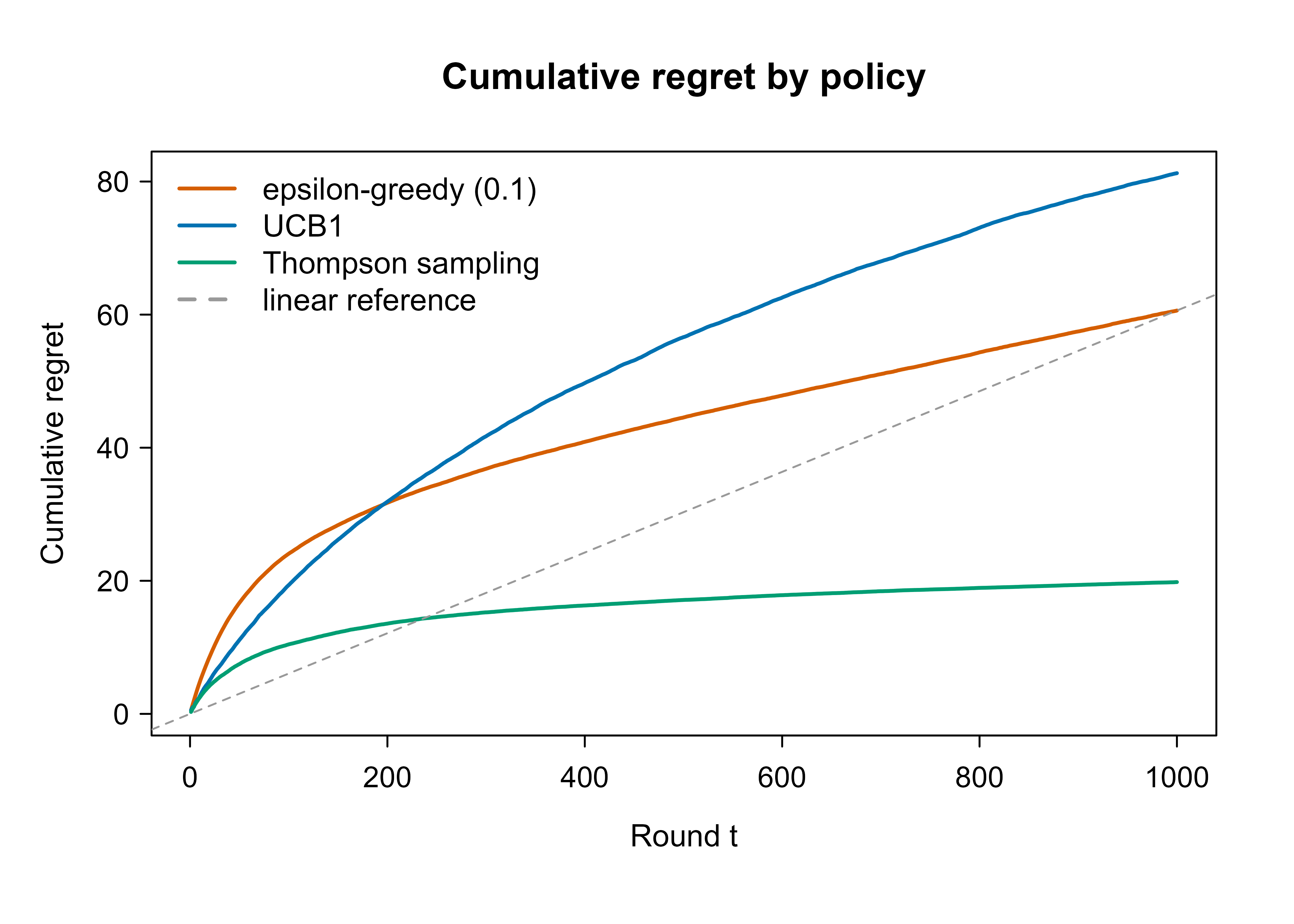
Figure 65.1 shows the average cumulative regret of the three policies as a function of the round \(t\). A flatter curve is better: it means the policy stopped paying for mistakes. The dashed grey line is the linear-regret reference that epsilon-greedy with a fixed \(\varepsilon\) trends toward, since it never stops exploring at a constant rate.

tt <- seq_len(horizon)
ymax <- max(reg_eps, reg_ucb, reg_ts)

plot(tt, reg_eps, type = "l", lwd = 2, col = "#D55E00",
     xlab = "Round t", ylab = "Cumulative regret",
     main = "Cumulative regret by policy",
     ylim = c(0, ymax))
lines(tt, reg_ucb, lwd = 2, col = "#0072B2")
lines(tt, reg_ts,  lwd = 2, col = "#009E73")

# Linear-regret reference line through the epsilon-greedy endpoint.
abline(a = 0, b = reg_eps[horizon] / horizon, lty = 2, col = "grey60")

legend("topleft", bty = "n", lwd = 2,
       col = c("#D55E00", "#0072B2", "#009E73", "grey60"),
       lty = c(1, 1, 1, 2),
       legend = c("epsilon-greedy (0.1)", "UCB1", "Thompson sampling",
                  "linear reference"))

Figure 65.1: Average cumulative regret over 200 runs for a 5-armed Bernoulli bandit (best arm value 0.75, horizon 1000). UCB and Thompson sampling bend toward sublinear (logarithmic) growth, while fixed epsilon-greedy keeps accruing regret at a roughly constant rate.

The two directed-exploration methods (UCB and Thompson sampling) flatten out as they zero in on the best arm, while epsilon-greedy keeps climbing in a near-straight line because its \(10\%\) random exploration never switches off.

65.7.2 Summary table

Table 65.1 reports, for each policy, the total cumulative regret at the horizon, the average reward per round, and the percentage of rounds in which the best arm was actually played. The optimal-play percentage is the clearest single diagnostic: a good policy converges to pulling the best arm almost every round.

# Re-run once per policy tracking which arm was best to compute "% optimal".
optimal_arm <- which.max(true_p)

summarize_policy <- function(policy_step_and_arm) {
  opt_hits <- numeric(n_runs)
  total_reward <- numeric(n_runs)
  final_regret <- numeric(n_runs)
  for (i in seq_len(n_runs)) {
    out <- policy_step_and_arm()
    opt_hits[i]     <- mean(out$arms == optimal_arm)
    total_reward[i] <- sum(out$reward)
    final_regret[i] <- sum(out$regret)
  }
  c(final_regret = mean(final_regret),
    reward_per_round = mean(total_reward) / horizon,
    pct_optimal = 100 * mean(opt_hits))
}

# Variants that also record the chosen arm and reward each step.
eg_track <- function(epsilon = 0.1) {
  Q <- rep(0, k); N <- rep(0, k)
  arms <- integer(horizon); reward <- numeric(horizon); regret <- numeric(horizon)
  for (t in seq_len(horizon)) {
    a <- if (runif(1) < epsilon) sample.int(k, 1) else which.max(Q)
    r <- pull(a); N[a] <- N[a] + 1; Q[a] <- Q[a] + (r - Q[a]) / N[a]
    arms[t] <- a; reward[t] <- r; regret[t] <- q_star - true_p[a]
  }
  list(arms = arms, reward = reward, regret = regret)
}
ucb_track <- function(c = sqrt(2)) {
  Q <- rep(0, k); N <- rep(0, k)
  arms <- integer(horizon); reward <- numeric(horizon); regret <- numeric(horizon)
  for (t in seq_len(horizon)) {
    a <- if (any(N == 0)) which(N == 0)[1] else which.max(Q + c * sqrt(log(t) / N))
    r <- pull(a); N[a] <- N[a] + 1; Q[a] <- Q[a] + (r - Q[a]) / N[a]
    arms[t] <- a; reward[t] <- r; regret[t] <- q_star - true_p[a]
  }
  list(arms = arms, reward = reward, regret = regret)
}
ts_track <- function() {
  alpha <- rep(1, k); beta_ <- rep(1, k)
  arms <- integer(horizon); reward <- numeric(horizon); regret <- numeric(horizon)
  for (t in seq_len(horizon)) {
    a <- which.max(rbeta(k, alpha, beta_))
    r <- pull(a); alpha[a] <- alpha[a] + r; beta_[a] <- beta_[a] + (1 - r)
    arms[t] <- a; reward[t] <- r; regret[t] <- q_star - true_p[a]
  }
  list(arms = arms, reward = reward, regret = regret)
}

set.seed(7)
summary_tab <- rbind(
  `epsilon-greedy (0.1)` = summarize_policy(function() eg_track(0.1)),
  `UCB1`                 = summarize_policy(function() ucb_track(sqrt(2))),
  `Thompson sampling`    = summarize_policy(ts_track)
)
summary_df <- data.frame(
  Policy             = rownames(summary_tab),
  `Final regret`     = round(summary_tab[, "final_regret"], 1),
  `Reward / round`   = round(summary_tab[, "reward_per_round"], 3),
  `% optimal pulls`  = round(summary_tab[, "pct_optimal"], 1),
  check.names = FALSE, row.names = NULL
)

knitr::kable(
  summary_df,
  caption = "Performance over 200 runs (horizon 1000). Lower final regret is better; reward per round and the share of rounds that played the best arm (true best value 0.75) are higher-is-better. Thompson sampling leads on all three measures. UCB still pays a visible exploration cost at this short horizon, the price of the log t bonus that buys it the lower asymptotic regret rate."
)

Table 65.1: Performance over 200 runs (horizon 1000). Lower final regret is better; reward per round and the share of rounds that played the best arm (true best value 0.75) are higher-is-better. Thompson sampling leads on all three measures. UCB still pays a visible exploration cost at this short horizon, the price of the log t bonus that buys it the lower asymptotic regret rate.

Policy	Final regret	Reward / round	% optimal pulls
epsilon-greedy (0.1)	59.9	0.691	82.3
UCB1	82.2	0.669	73.0
Thompson sampling	21.2	0.729	92.8

Thompson sampling reaches the best arm on the largest share of rounds and leaves the least regret on the table. UCB’s final regret is higher than epsilon-greedy’s at this horizon of \(1000\): its exploration bonus is still actively probing uncertain arms early on, which is exactly the investment that gives it logarithmic (rather than linear) regret as the horizon grows. Extend the run and the UCB curve flattens while a fixed-\(\varepsilon\) curve keeps rising, so the ranking eventually reverses. This is a useful reminder that asymptotic guarantees and short-horizon behavior can disagree.

65.8 Practical guidance and pitfalls

The choice among these methods is rarely about asymptotic regret bounds, since UCB and Thompson sampling share the same logarithmic rate. It is about engineering fit. Thompson sampling is usually the first thing to reach for: it is a few lines of code for Bernoulli arms, it has no tuning constant to set, it tends to win empirically, and its randomized choices spread load naturally across a fleet of servers. UCB is attractive when you want a deterministic, auditable rule (useful when a decision must be explained or reproduced) and when you can tolerate tuning the exploration constant \(c\). Epsilon-greedy earns its place as a baseline and in short-horizon or rapidly-drifting problems where its constant exploration is a feature rather than a bug.

Several traps catch people moving from the textbook to a real system.

Warning

A fixed \(\varepsilon\) gives linear regret. If you use epsilon-greedy for a long-running system, decay \(\varepsilon\) over time (for example \(\varepsilon_t = \min(1, c/t)\)) or accept that you are paying a permanent exploration tax.

The first trap is nonstationarity. All the regret guarantees here assume arm values are fixed. Real click-through rates drift with the season, the news cycle, and the user population. A sample mean \(Q_t(a)\) that averages over all of history responds ever more sluggishly to change, since each new reward moves it by only \(1/N_t(a)\). The fix is to forget the distant past: use a constant step size, \(Q_{n+1} = Q_n + \beta(R_{n+1} - Q_n)\) with fixed \(\beta \in (0,1)\), or a sliding window. For Thompson sampling, apply a small decay to the Beta counts each round so old evidence fades.

The second trap is delayed feedback. The clean model assumes the reward for round \(t\) arrives before round \(t+1\). In practice a conversion may take hours to register, so the algorithm chooses many arms before learning their outcomes. Batched and delayed-feedback variants exist; the practical rule of thumb is that more delay means you should explore a little more, because your estimates lag reality.

The third trap is non-binary or unbounded rewards. UCB1 as derived assumes rewards in \([0,1]\) (that bound is what makes Hoeffding’s inequality apply). If your reward is revenue in dollars, either scale it into \([0,1]\) using a known maximum or switch to a variant designed for sub-Gaussian rewards. For Thompson sampling, replace the Beta-Bernoulli pair with the conjugate model that matches your reward distribution.

A final, easy mistake is evaluating a bandit like an A/B test. A bandit deliberately stops sampling the losing arms, so by the end of a run you have very little data on the arms it abandoned, and a naive significance test on that imbalanced data is misleading. If you need both to optimize and to draw rigorous statistical conclusions about every arm, look at off-policy evaluation and explore/exploit designs built for inference, not at the raw bandit logs.

65.9 Connection to contextual bandits and reinforcement learning

The bandits in this chapter are context-free: the best arm is the same on every round. Add a feature vector \(x_t\) that arrives before each choice and lets the best arm vary by situation (this user, this time of day) and you have a contextual bandit, the subject of the contextual bandits chapter (Chapter 72). The three strategies here carry over directly: epsilon-greedy still flips a coin, UCB becomes LinUCB by putting a confidence ellipsoid around a linear reward model, and Thompson sampling places a posterior over the model parameters instead of over a single value per arm.

Go one step further and let your action change the state of the world, so that today’s choice affects tomorrow’s options, and you have left bandits entirely for full reinforcement learning (Chapter 64), where the action-value update gains a term for future reward. The incremental update \(Q \leftarrow Q + \alpha(\text{target} - Q)\) you met in this chapter is precisely the seed that grows into temporal-difference learning and Q-learning (Chapter 66).

65.10 Further reading

The standard textbook treatment, and the source of the action-value and incremental-update framing used here, is Sutton and Barto, Reinforcement Learning: An Introduction, 2nd edition (2018), especially Chapter 2. A thorough, modern, theory-focused reference is Lattimore and Szepesvari, Bandit Algorithms (2020). The classics worth knowing by name are Robbins (1952) for the original formulation, Lai and Robbins (1985) for the logarithmic regret lower bound, Auer, Cesa-Bianchi, and Fischer (2002) for UCB1, Thompson (1933) for the sampling method that now bears his name, and Agrawal and Goyal (2012) for its modern regret analysis. Russo, Van Roy, Kazerouni, Osband, and Wen, “A Tutorial on Thompson Sampling” (2018), is an accessible deep dive on the Bayesian approach.

---

1. The earliest formal treatment is usually credited to Robbins (1952), though the problem was discussed during the Second World War as a model for allocating effort across competing research projects.