A single decision tree is easy to read but hard to trust: change a few training points and the tree can split on a completely different variable, sending its predictions in a new direction. Trees are, in the language of the bias-variance tradeoff, low bias but high variance learners. Bagging (Chapter 10) already addresses this by growing many trees on bootstrap resamples and averaging them, which knocks down variance without raising bias much. Random forests push that idea one step further. They start from bagging and add a single, almost embarrassingly simple twist that turns out to matter a great deal: at every split, each tree is only allowed to look at a random handful of the predictors.
In this chapter you will learn why that twist works (it is a story about correlation, not about individual trees getting better), how the algorithm is put together step by step, how to read its built-in error estimate and variable-importance scores, and how to fit and tune one in R. Random forests are a strong default for general nonlinear, nonparametric prediction, so this is a method worth understanding well before reaching for anything fancier.
Intuition
Bagging averages many trees, but if those trees all key on the same one or two dominant predictors, they make correlated mistakes, and averaging correlated things barely helps. Random forests force the trees to disagree by hiding most of the predictors at each split. The trees become more diverse, their errors cancel more effectively, and the average is more stable.
13.1 From bagging to decorrelated trees
Random forests are a bootstrap-based procedure built on a committee of trees, exactly like bagging (Chapter 10). The difference is that random forests deliberately decorrelate the trees. At each split in the tree-building process, and separately for each bootstrap sample, the splitting rule is chosen from a randomly selected, relatively small subset of the input variables. Because different variables are available at different splits and in different trees, the trees stop leaning on the same dominant covariates and become much less dependent on one another. That reduced dependence is what reduces the variance of the final prediction.
This variance reduction is the whole point. Trees are inherently noisy, but when grown fairly deep they have relatively low bias. Averaging many low-bias, nearly independent trees therefore gives predictions (or classifications) that keep the low bias while shedding most of the variance.
To see why correlation is the villain, recall a basic fact about averaging: the variance of an average of correlated variables is larger than the variance of an average of the same number of independent variables.1 Concretely, the average of \(B\) identically distributed random variables, each with variance \(\sigma^2\) and pairwise correlation \(\rho\), has variance
Look at what happens as the forest grows. The second term, \(\sigma^2 (1 - \rho)/B\), shrinks to zero as \(B \to \infty\), but the first term, \(\rho \sigma^2\), does not depend on \(B\) at all. No matter how many trees you add, the variance cannot fall below this floor of \(\rho \sigma^2\).
13.1.1 Deriving the variance of the average
It is worth deriving Equation 13.1 carefully, because the entire rationale for random forests rests on it. Let \(T_1, \dots, T_B\) be the predictions of the individual trees at a fixed input \(x\), treated as random variables over the draw of the bootstrap samples and the split randomness \(\Theta_b\). Assume they are identically distributed (not independent) with common variance \(\operatorname{Var}(T_b) = \sigma^2\) and common pairwise correlation \(\operatorname{Corr}(T_b, T_{b'}) = \rho\) for \(b \ne b'\), so that \(\operatorname{Cov}(T_b, T_{b'}) = \rho \sigma^2\). The forest prediction is \(\bar T = \frac{1}{B}\sum_{b=1}^B T_b\). Expanding the variance of a sum into its \(B\) diagonal (variance) terms and \(B(B-1)\) off-diagonal (covariance) terms,
which is exactly Equation 13.1. The derivation makes the mechanism transparent: smaller \(m\) removes shared dominant predictors from many splits, lowering the off-diagonal covariance \(\rho\sigma^2\) and hence the irreducible floor, but pushing \(m\) too small also raises each tree’s own variance \(\sigma^2\) and its bias, since each split now chooses from a weaker pool of candidate variables. The optimal \(m\) trades these two effects off, which is why it is tuned rather than fixed.
A subtlety about the correlation
The relevant \(\rho\) is the correlation between the predictions of two forest trees at the same test point \(x\), induced by their shared training data, not the sampling correlation of an estimator across independent data sets. As \(B\) grows, \(\bar T(x)\) converges almost surely to its expectation \(\mathbb{E}_\Theta[T(x;\Theta)]\) over the randomization, so \(B\) is not a tuning parameter in the usual sense: more trees only ever help (up to Monte Carlo noise) and never overfit. The bound Equation 13.2 is what guarantees this.
We can confirm Equation 13.2 numerically with a small base-R simulation. We generate \(B\) correlated Gaussian variables with variance \(\sigma^2\) and pairwise correlation \(\rho\), average them, repeat many times, and compare the empirical variance of the average to the formula.
The two numbers agree to Monte Carlo error, and increasing B drives the average’s variance toward the floor rho * sigma2 = 1.2, never below it.
Key idea
Adding more trees only attacks the \(\sigma^2(1-\rho)/B\) part of the variance. The floor \(\rho \sigma^2\) can only be lowered by reducing the correlation \(\rho\) between trees. Random forests lower \(\rho\) by randomizing the variables available at each split, which is precisely the dependence that plain bagging (Chapter 10) leaves in place.
13.2 The algorithm
Before the formal statement, here is the idea in four plain steps:
Create bootstrapped datasets (sampling with replacement).
Grow a decision tree on each bootstrapped dataset, but at every split consider only a random subset of the variables.
Repeat steps 1 and 2 many times to build a whole forest.
To predict, run a new observation through every tree and combine the results: average them for regression, or take a majority vote for classification (the same aggregation idea as in bagging (Chapter 10), applied to many bootstrap samples).
The one new knob compared to bagging is \(m\), the number of input variables made available at each split, where \(m \le p\) and \(p\) is the total number of predictors. Smaller \(m\) means more aggressive decorrelation. There is no theory that pins down the best value, but two rules of thumb, supported by simulation studies rather than by any deeper result, work well as starting points:
\(m = \sqrt{p}\) for classification.
\(m = \frac{p}{3}\) for regression.
After \(B\) trees are grown, \(\{T(x, \Theta_b)\}^B_1\), the random forest regression predictor is the simple average of the trees,
Draw a bootstrap sample \(\mathbf{Z}^*\) of size N from the training data.
Grow a random-forest tree \(T_b\) on the bootstrapped data by recursively repeating the following steps at each terminal node, until the minimum node size \(n_{min}\) is reached:
Select \(m\) variables at random from the \(p\) variables.
Pick the best variable and split-point among those \(m\).
Split the node into two daughter nodes.
Output the ensemble of trees \(\{T_b\}^B_1\).
To predict at a new point \(x\), the two tasks differ only in how the trees are combined:
Classification: let \(\hat{C}_b (x)\) be the class predicted by the \(b\)-th tree. Then \(\hat{C}_{rf}^B (x) = \text{majority vote } \{\hat{C}_b (x) \}^B_{1}\).
Note
Random subset selection happens at every split, not once per tree. A fresh random set of \(m\) variables is drawn each time a node is split, which is what keeps even the same tree from being dominated by one strong predictor.
How does this compare to its neighbors? In general, gradient boosting (Chapter 12) is roughly comparable to random forests, and random forests usually beat plain bagging (Chapter 10), though in practice these orderings do not always hold. Which method wins depends on the structure of the problem: the degree of linearity or nonlinearity, the dependence among covariates, the relative importance of specific predictors, and so on.
When to use this
Reach for a random forest when you want strong nonlinear, nonparametric prediction with little tuning, mixed variable types, and a built-in honest error estimate. If you need to squeeze out the last bit of accuracy on highly structured data, compare against gradient boosting (Chapter 12).
13.3 Out-of-bag error: free cross-validation
A pleasant side effect of bootstrapping is that the forest comes with its own validation set. Each bootstrap sample leaves out roughly a third of the observations, and those left-out points are called the out-of-bag (OOB) samples for that tree.
For each observation pair \((x_i, y_i)\), we can form an OOB prediction by averaging only the trees built on bootstrap samples in which that observation did not appear. Comparing these OOB predictions to the actual responses gives the OOB error, which behaves like a cross-validation error estimate but costs nothing extra to compute. A useful practical signal falls out of this: once the OOB error stops improving as you add trees, the forest has effectively converged and more trees will not help.
13.3.1 Why roughly a third is left out
The “roughly a third” is not a heuristic; it follows from the bootstrap. A bootstrap sample draws \(N\) points with replacement from a training set of size \(N\), so each draw selects observation \(i\) with probability \(1/N\). The probability that observation \(i\) is missed on all \(N\) draws is
using \(\lim_{N\to\infty}(1 - 1/N)^N = e^{-1}\). Hence about \(36.8\%\) of observations are out-of-bag for any given tree, and a given observation is OOB for, in expectation, a fraction \(e^{-1}\) of the \(B\) trees, leaving on the order of \(0.368\,B\) trees to form its OOB prediction. Because the OOB prediction of \((x_i, y_i)\) uses only trees that never saw that point, the OOB error is a genuine held-out estimate of generalization error. As \(B \to \infty\) it is asymptotically equivalent to leave-one-out cross-validation over the bootstrap distribution, which is why it can replace a manually held-out test set.
When OOB error is optimistic or unstable
The OOB estimate degrades when the number of trees is small (each point then has very few OOB trees, so its prediction is noisy) and when observations are not independent, for example with spatial, temporal, or grouped data. In the latter case bootstrap resampling does not break the dependence between in-bag and out-of-bag points, and the OOB error can be badly optimistic, just as ordinary cross-validation is when folds share dependent records.
Tip
Watch the OOB error as a function of the number of trees. When the curve flattens, you have enough trees. This is the random forest equivalent of a learning curve, and you get it without holding out a separate set.
13.4 Variable importance
Because each split sees a random subset of predictors, random forests give variables that would otherwise be overshadowed a chance to be chosen. As a result, the forest tends to surface more “important” variables than a single greedy tree would. There are two common ways to score importance.
The first measures, for each variable, how much it improves the split criterion (such as node impurity) summed and averaged across all trees. Variables that produce big, frequent improvements score high. Formally, let a split \(s\) at an internal node \(t\) send a fraction \(p_L\) of the node’s samples left and \(p_R = 1 - p_L\) right, and let \(i(\cdot)\) be the node impurity (Gini index or entropy for classification, residual sum of squares for regression). The impurity decrease at that node is
weighted by the proportion of samples reaching \(t\). The mean decrease in impurity (MDI) importance of variable \(j\) is the sum of these weighted decreases over all nodes that split on \(j\), averaged over the \(B\) trees. MDI is essentially free, since the quantities are already computed during training, but it is biased: it inflates the apparent importance of high-cardinality categorical variables and continuous variables, which offer more candidate split points and thus more chances to reduce impurity even by chance.
The second is permutation importance, which is based on OOB prediction. When the \(b\)-th tree is grown, its OOB samples are passed down the tree and the prediction accuracy is recorded. The values of the \(j\)-th variable are then randomly permuted across those OOB samples, breaking any relationship between that variable and the response, and the accuracy is recomputed. The drop in accuracy, averaged over all trees, measures the importance of variable \(j\). Writing \(\mathrm{OOB}_b\) for the out-of-bag set of tree \(b\) and \(\pi_j\) for a random permutation of the \(j\)-th coordinate within that set, the permutation importance is
where \(\mathrm{err}_b\) is the tree’s OOB error (misclassification rate or mean squared error). Because the comparison is made on held-out data with the model fixed, Equation 13.5 measures how much the fitted forest actually relies on \(X_j\) for prediction, which is a different and usually more trustworthy question than MDI’s “how often did \(X_j\) get chosen during training.”
Correlated predictors distort both scores
When two predictors are strongly correlated, the forest can split on either one, so neither looks individually indispensable and both can receive deflated permutation scores even though the pair is jointly important. Permuting a variable marginally also generates feature combinations that never occur in the data (extrapolation), which can make the importance unstable. Conditional permutation importance and grouped or drop-and-relearn schemes address these failure modes at higher computational cost.
Warning
Permutation importance does not tell you how the model would do if that variable were simply unavailable. A refit model would likely lean on correlated surrogate variables to fill the gap, so dropping a “high importance” variable may hurt far less than its score suggests.
13.5 Other properties to keep in mind
A few additional points round out the picture of how random forests behave in practice:
Proximity plots show which observations the forest treats as effectively close together. They are useful mainly for seeing where points sit relative to the decision boundary; we use this idea in the application below to build an MDS plot.
Overfitting: random forests are fairly robust to overfitting when the number of genuinely relevant variables in \(X\) is large relative to \(p\).
Bias: the bias of a random forest is essentially the same as the bias of an individual tree. The gain in mean squared error comes entirely from variance reduction, not from lower bias.
Relationship to other methods: a random forest behaves somewhat like a nearest-neighbor classifier (such as \(k\)-nearest neighbor; see Chapter 17), since predictions are driven by training points that fall in the same regions.
Software: common implementations include randomForest, cforest, ParallelForest, ranger, and Rborist.
In short, random forests are a reliable, low-maintenance tool for general nonlinear, nonparametric prediction. With the mechanics in hand, the rest of the chapter walks through a complete worked example.
13.6 Statistical properties
This section collects the theoretical facts that justify the method, going beyond the variance argument of Chapter 13.
13.6.1 Bias-variance decomposition of the ensemble
Fix a test point \(x\) and write the forest estimate as \(\hat f_{rf}(x) = \mathbb{E}_\Theta[T(x;\Theta)]\) in the infinite-tree limit (averaging over the randomization \(\Theta\) for a fixed training set, then over training sets). For squared-error loss the usual decomposition holds,
Two facts make random forests work. First, averaging is a linear operation, so the bias of the ensemble equals the bias of a single randomized tree: \(\mathbb{E}[\hat f_{rf}(x)] = \mathbb{E}_\Theta\mathbb{E}[T(x;\Theta)]\), and randomizing the candidate variables does not change the expected fitted function by much when trees are grown deep. This is the precise sense of the chapter’s earlier remark that the forest’s bias is essentially that of one tree. Second, the variance term is exactly Equation 13.2 and is driven down toward its floor \(\rho\sigma^2\) by decorrelation. The entire MSE gain over a single tree comes from the variance term; the price of decorrelation is a slight increase in \(\sigma^2\) and bias as \(m\) shrinks, which is why very small \(m\) can underperform.
13.6.2 Consistency and rates
Random forests are nonparametric estimators, and consistency results require care because the bootstrap and the data-dependent splits make the trees hard to analyze. Two routes are standard. For centered or purely random forests, whose splits are chosen independently of \(Y\), one can show \(L^2\) consistency, \(\mathbb{E}[(\hat f_{rf}(X) - f(X))^2] \to 0\), under mild smoothness of \(f\), with rates governed by the effective number of cells. The convergence rate is the nonparametric rate \(n^{-2/(2 + d)}\) for a \(d\)-dimensional Lipschitz target in the worst case, slower as \(d\) grows (the curse of dimensionality), but the rate adapts to a smaller intrinsic dimension when only a few of the \(p\) inputs are relevant, which is the regime where forests shine. For Breiman’s original CART-split forests, whose splits depend on \(Y\) and are far harder to analyze, consistency has been established under an additive-model assumption (Scornet, Biau, and Vert, 2015). The practical message is that forests are consistent under reasonable conditions but converge at nonparametric rates, so they cannot escape the curse of dimensionality when the truth genuinely depends on many interacting variables.
13.6.3 Connection to adaptive nearest neighbors and kernels
A forest prediction can be written as a weighted average of the training responses,
where \(L_b(x)\) is the terminal node (“leaf”) of tree \(b\) containing \(x\) and \(|L_b(x)|\) is the number of training points in it. The weight \(w_i(x)\) is large when \(x_i\) falls in the same leaf as \(x\) in many trees, which is exactly the proximity used for the MDS plot in the application. Equation Equation 13.7 shows a random forest is an adaptive nearest-neighbor or kernel method: it defines a data-driven similarity \(w_i(x)\) that, unlike fixed-bandwidth \(k\)-nearest neighbors (Chapter 17), stretches and shrinks the neighborhood along directions the trees deem relevant. This view also yields quantile and survival forests (predict a weighted quantile or weighted Kaplan-Meier curve using the same \(w_i\)) and underlies the infinitesimal-jackknife and U-statistic variance estimators for forest predictions.
13.6.4 Computational and sample complexity
Building one tree costs \(O(\tilde m\, N \log N)\) in the typical balanced case, where \(\tilde m\) is the number of candidate variables evaluated per node (here \(m\)) and the \(N \log N\) comes from sorting or scanning \(N\) points down a tree of depth \(O(\log N)\); the full forest is \(O(B\, m\, N \log N)\). Memory is \(O(B \times \text{nodes per tree})\), which can be substantial for deep trees on large \(N\). Prediction costs \(O(B \log N)\) per query, since each query traverses \(B\) trees of depth \(O(\log N)\). The trees are independent, so both training and prediction are embarrassingly parallel across the \(B\) trees, which is why packages such as ranger scale well across cores. Reducing \(m\) reduces per-node work linearly, an underappreciated reason small \(m\) is fast as well as more decorrelated.
13.6.5 Failure modes
Random forests break or underperform in identifiable situations. They cannot extrapolate: because every prediction is a weighted average of observed \(y_i\) via Equation 13.7, predictions are bounded by the range of the training responses, so a forest will systematically under- or over-predict beyond the training support and is a poor choice for strongly trending time series. They are inefficient on sparse high-dimensional problems where most of \(p\) is noise, since with small \(m\) a relevant variable is rarely even offered at a split; some implementations counter this with informed sampling of candidate variables. Smooth or strongly linear signals are fit with axis-aligned step functions, so a forest needs many trees to approximate a simple linear surface that a linear model captures exactly. Finally, default settings can overfit noisy classification when classes are imbalanced; class weights, stratified bootstrap sampling, or balanced subsampling are the usual remedies.
13.7 Application
To make the ideas concrete, we walk through a complete classification example: predicting whether a patient has heart disease. Along the way we will impute missing values, fit a forest, read its OOB error, tune \(m\) (called mtry in the code), and visualize the patients with a proximity-based plot. The example follows a demo by Josh Starmer2.
We start by loading the packages we need: ggplot2 and cowplot for plotting, and randomForest for the model itself.
The raw file arrives with no column names and a few quirks, so before modeling we reformat it for two reasons: to make it easy to read by giving the columns meaningful names, and to make sure randomForest interprets each variable correctly (factors as factors, missing values as NA rather than the literal string "?"). The comments below document what each clinical variable means.
Show code
head(data)# you see data, but no column names#> V1 V2 V3 V4 V5 V6 V7 V8 V9 V10 V11 V12 V13 V14#> 1 63 1 1 145 233 1 2 150 0 2.3 3 0.0 6.0 0#> 2 67 1 4 160 286 0 2 108 1 1.5 2 3.0 3.0 2#> 3 67 1 4 120 229 0 2 129 1 2.6 2 2.0 7.0 1#> 4 37 1 3 130 250 0 0 187 0 3.5 3 0.0 3.0 0#> 5 41 0 2 130 204 0 2 172 0 1.4 1 0.0 3.0 0#> 6 56 1 2 120 236 0 0 178 0 0.8 1 0.0 3.0 0colnames(data)<-c("age","sex",# 0 = female, 1 = male"cp", # chest pain # 1 = typical angina, # 2 = atypical angina, # 3 = non-anginal pain, # 4 = asymptomatic"trestbps", # resting blood pressure (in mm Hg)"chol", # serum cholestoral in mg/dl"fbs", # fasting blood sugar if less than 120 mg/dl, 1 = TRUE, 0 = FALSE"restecg", # resting electrocardiographic results# 1 = normal# 2 = having ST-T wave abnormality# 3 = showing probable or definite left ventricular hypertrophy"thalach", # maximum heart rate achieved"exang", # exercise induced angina, 1 = yes, 0 = no"oldpeak", # ST depression induced by exercise relative to rest"slope", # the slope of the peak exercise ST segment # 1 = upsloping # 2 = flat # 3 = downsloping "ca", # number of major vessels (0-3) colored by fluoroscopy"thal", # this is short of thalium heart scan# 3 = normal (no cold spots)# 6 = fixed defect (cold spots during rest and exercise)# 7 = reversible defect (when cold spots only appear during exercise)"hd"# (the predicted attribute) - diagnosis of heart disease # 0 if less than or equal to 50% diameter narrowing# 1 if greater than 50% diameter narrowing)# head(data) # now we have data and column names# str(data) # this shows that we need to tell R which columns contain factors# it also shows us that there are some missing values. There are "?"s# in the dataset.## First, replace "?"s with NAs.data[data=="?"]<-NA## Now add factors for variables that are factors and clean up the factors## that had missing data...data[data$sex==0,]$sex<-"F"data[data$sex==1,]$sex<-"M"data$sex<-as.factor(data$sex)data$cp<-as.factor(data$cp)data$fbs<-as.factor(data$fbs)data$restecg<-as.factor(data$restecg)data$exang<-as.factor(data$exang)data$slope<-as.factor(data$slope)data$ca<-as.integer(data$ca)# since this column had "?"s in it (which# we have since converted to NAs) R thinks that# the levels for the factor are strings, but# we know they are integers, so we'll first# convert the strings to integers...data$ca<-as.factor(data$ca)# ...then convert the integers to factor levelsdata$thal<-as.integer(data$thal)# "thal" also had "?"s in it.data$thal<-as.factor(data$thal)## This next line replaces 0 and 1 with "Healthy" and "Unhealthy"data$hd<-ifelse(test=data$hd==0, yes="Healthy", no="Unhealthy")data$hd<-as.factor(data$hd)# Now convert to a factorstr(data)## this shows that the correct columns are factors and we've replaced#> 'data.frame': 303 obs. of 14 variables:#> $ age : num 63 67 67 37 41 56 62 57 63 53 ...#> $ sex : Factor w/ 2 levels "F","M": 2 2 2 2 1 2 1 1 2 2 ...#> $ cp : Factor w/ 4 levels "1","2","3","4": 1 4 4 3 2 2 4 4 4 4 ...#> $ trestbps: num 145 160 120 130 130 120 140 120 130 140 ...#> $ chol : num 233 286 229 250 204 236 268 354 254 203 ...#> $ fbs : Factor w/ 2 levels "0","1": 2 1 1 1 1 1 1 1 1 2 ...#> $ restecg : Factor w/ 3 levels "0","1","2": 3 3 3 1 3 1 3 1 3 3 ...#> $ thalach : num 150 108 129 187 172 178 160 163 147 155 ...#> $ exang : Factor w/ 2 levels "0","1": 1 2 2 1 1 1 1 2 1 2 ...#> $ oldpeak : num 2.3 1.5 2.6 3.5 1.4 0.8 3.6 0.6 1.4 3.1 ...#> $ slope : Factor w/ 3 levels "1","2","3": 3 2 2 3 1 1 3 1 2 3 ...#> $ ca : Factor w/ 4 levels "0","1","2","3": 1 4 3 1 1 1 3 1 2 1 ...#> $ thal : Factor w/ 3 levels "3","6","7": 2 1 3 1 1 1 1 1 3 3 ...#> $ hd : Factor w/ 2 levels "Healthy","Unhealthy": 1 2 2 1 1 1 2 1 2 2 ...## "?"s with NAs because "?" no longer appears in the list of factors## for "ca" and "thal"
With the data cleaned and typed correctly, we are ready to build a forest. This is a good moment to recall the OOB idea from earlier in the chapter, because it changes how we set up the example.
Note
Most machine learning methods require you to split the data manually into a training set and a test set, so you can train on one part and evaluate on data the model never saw. Random forests do this splitting for you. Because each tree is built on a bootstrap sample, not every observation is used in every tree: the bootstrap sample plays the role of the training data, and the left-out observations, the out-of-bag (OOB) data, play the role of the test set. That is why the example below never carves out a separate test set by hand.
We also have missing values to deal with. Rather than drop incomplete rows, we impute them using rfImpute, which fills in missing entries based on random forest proximities (how similar observations are according to a preliminary forest). Breiman suggests 4 to 6 iterations is usually enough, so we use iter = 6.
Show code
set.seed(42)## impute any missing values in the training set using proximitiesdata.imputed<-rfImpute(hd~., data =data, iter=6)#> ntree OOB 1 2#> 300: 17.49% 12.80% 23.02%#> ntree OOB 1 2#> 300: 16.83% 14.02% 20.14%#> ntree OOB 1 2#> 300: 17.82% 13.41% 23.02%#> ntree OOB 1 2#> 300: 17.49% 14.02% 21.58%#> ntree OOB 1 2#> 300: 17.16% 12.80% 22.30%#> ntree OOB 1 2#> 300: 18.15% 14.63% 22.30%## NOTE: iter = the number of iterations to run. Breiman says 4 to 6 iterations## is usually good enough. With this dataset, when we set iter=6, OOB-error## bounces around between 17% and 18%. When we set iter=20,# set.seed(42)# data.imputed <- rfImpute(hd ~ ., data = data, iter=20)## we get values a little better and a little worse, so doing more## iterations doesn't improve the situation.#### NOTE: If you really want to micromanage how rfImpute(),## you can change the number of trees it makes (the default is 300) and the## number of variables that it will consider at each step.## Now we are ready to build a random forest.## NOTE: If the thing we're trying to predict (in this case it is## whether or not someone has heart disease) is a continuous number## (i.e. "weight" or "height"), then by default, randomForest() will set## "mtry", the number of variables to consider at each step,## to the total number of variables divided by 3 (rounded down), or to 1## (if the division results in a value less than 1).## If the thing we're trying to predict is a "factor" (i.e. either "yes/no"## or "ranked"), then randomForest() will set mtry to## the square root of the number of variables (rounded down to the next## integer value).## In this example, "hd", the thing we are trying to predict, is a factor and## there are 13 variables. So by default, randomForest() will set## mtry = sqrt(13) = 3.6 rounded down = 3## Also, by default random forest generates 500 trees (NOTE: rfImpute() only## generates 300 tress by default)model<-randomForest(hd~., data=data.imputed, proximity=TRUE)## RandomForest returns all kinds of thingsmodel# gives us an overview of the call, along with...#> #> Call:#> randomForest(formula = hd ~ ., data = data.imputed, proximity = TRUE) #> Type of random forest: classification#> Number of trees: 500#> No. of variables tried at each split: 3#> #> OOB estimate of error rate: 16.83%#> Confusion matrix:#> Healthy Unhealthy class.error#> Healthy 142 22 0.1341463#> Unhealthy 29 110 0.2086331# 1) The OOB error rate for the forest with ntree trees. # In this case ntree=500 by default# 2) The confusion matrix for the forest with ntree trees.# The confusion matrix is laid out like this:
Printing the model object gives a compact summary of the fit. Two pieces matter most: the OOB estimate of the error rate (here for the default ntree = 500 trees), which is our honest, cross-validation-like accuracy check, and the confusion matrix, which breaks the errors down by class. The confusion matrix is laid out like this, with true classes in the rows and predicted classes in the columns:
Healthy | Number of healthy people | Number of healthy people | | correctly called “healthy” | incorrectly called “unhealthy” | | by the forest. | by the forest | ————————————————————– Unhealthy| Number of unhealthy people | Number of unhealthy people | | incorrectly called | correctly called “unhealthy” | | “healthy” by the forest | by the forest | ————————————————————–
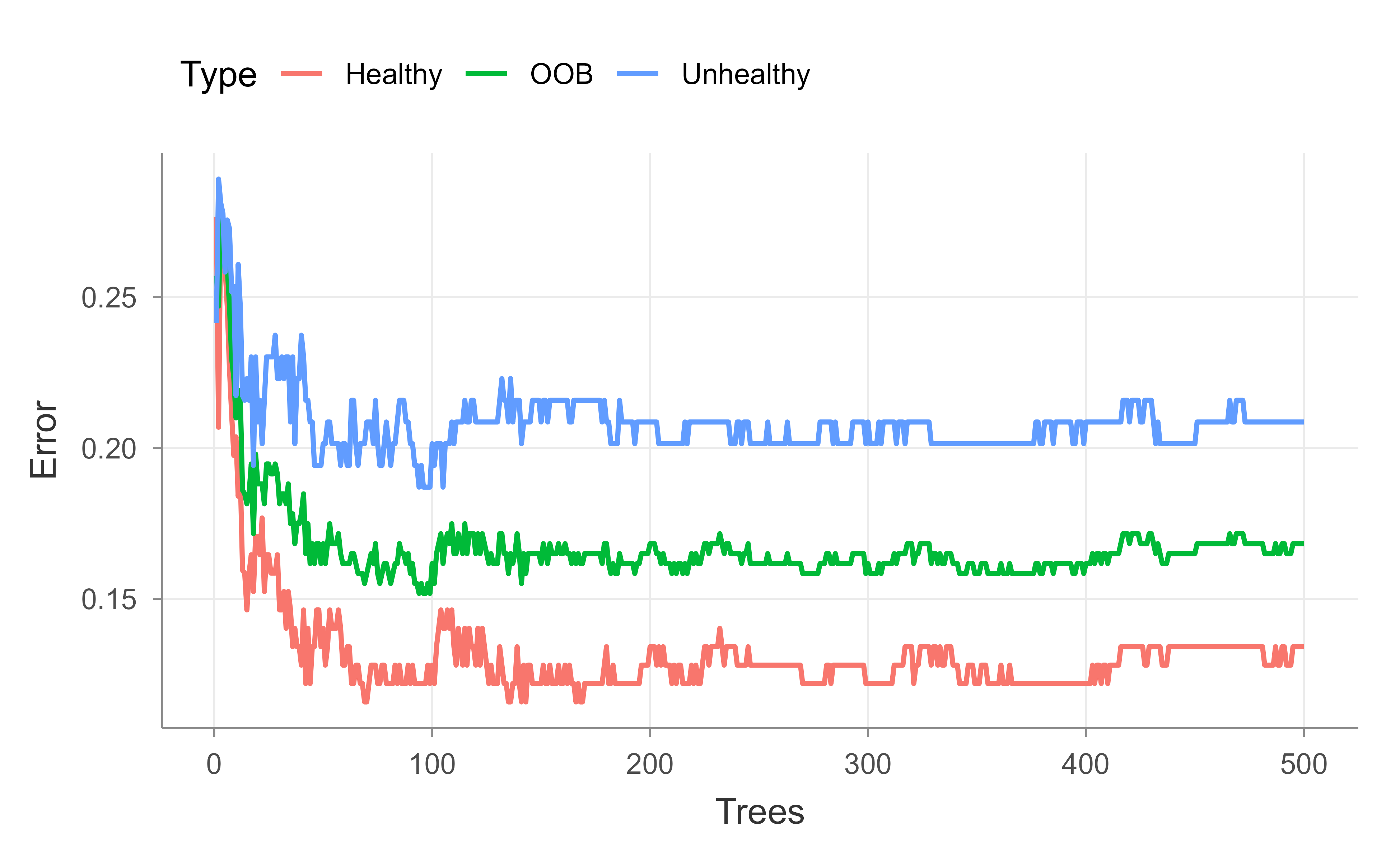
Next we check whether the forest has enough trees. The principle from earlier applies directly: up to a point, more trees help, and you know you have enough once the OOB error stops improving. We plot the OOB error against the number of trees, tracking the overall rate as well as the per-class rates, so we can watch for convergence. Figure 13.1 shows the result for the default 500-tree forest.
Show code
## Now check to see if the random forest is actually big enough...## Up to a point, the more trees in the forest, the better. You can tell when## you've made enough when the OOB no longer improves.oob.error.data<-data.frame( Trees=rep(1:nrow(model$err.rate), times=3), Type=rep(c("OOB", "Healthy", "Unhealthy"), each=nrow(model$err.rate)), Error=c(model$err.rate[,"OOB"],model$err.rate[,"Healthy"],model$err.rate[,"Unhealthy"]))ggplot(data=oob.error.data, aes(x=Trees, y=Error))+geom_line(aes(color=Type))# ggsave("oob_error_rate_500_trees.pdf")## Blue line = The error rate specifically for calling "Unheathly" patients that## are OOB.#### Green line = The overall OOB error rate.#### Red line = The error rate specifically for calling "Healthy" patients## that are OOB.
Figure 13.1: Out-of-bag error rate as a function of the number of trees for the 500-tree heart disease forest. The overall OOB rate is shown alongside the per-class rates for healthy and unhealthy patients.
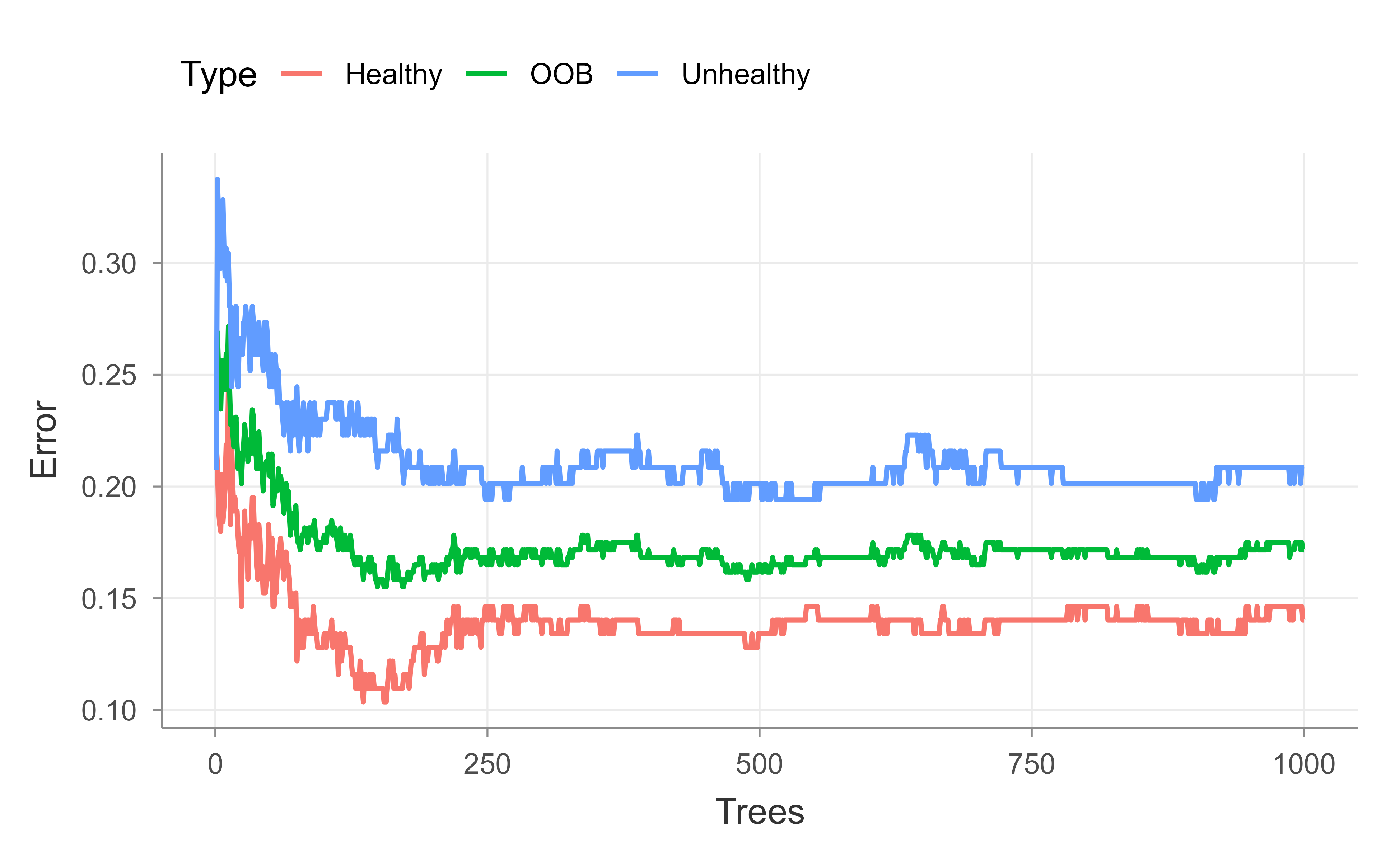
After building a random forest with 500 trees, the graph does not make it clear that the OOB error has settled on a value or, if we added more trees, whether it would continue to decrease. So we do the whole thing again, but this time add more trees. Figure 13.2 repeats the OOB curve for a 1,000-tree forest.
Show code
model<-randomForest(hd~., data=data.imputed, ntree=1000, proximity=TRUE)model#> #> Call:#> randomForest(formula = hd ~ ., data = data.imputed, ntree = 1000, proximity = TRUE) #> Type of random forest: classification#> Number of trees: 1000#> No. of variables tried at each split: 3#> #> OOB estimate of error rate: 17.16%#> Confusion matrix:#> Healthy Unhealthy class.error#> Healthy 141 23 0.1402439#> Unhealthy 29 110 0.2086331oob.error.data<-data.frame( Trees=rep(1:nrow(model$err.rate), times=3), Type=rep(c("OOB", "Healthy", "Unhealthy"), each=nrow(model$err.rate)), Error=c(model$err.rate[,"OOB"],model$err.rate[,"Healthy"],model$err.rate[,"Unhealthy"]))ggplot(data=oob.error.data, aes(x=Trees, y=Error))+geom_line(aes(color=Type))# ggsave("oob_error_rate_1000_trees.pdf")## After building a random forest with 1,000 trees, we get the same OOB-error## 16.5% and we can see convergence in the graph. So we could have gotten## away with only 500 trees, but we wouldn't have been sure that number## was enough.
Figure 13.2: Out-of-bag error rate as a function of the number of trees for the 1,000-tree heart disease forest. The curve flattens, showing that the OOB error has converged.
With 1,000 trees the OOB error lands at essentially the same value as with 500 and the curve clearly flattens, confirming that 500 trees would have been enough; we just could not be sure of that until we checked. Next we tune mtry, the number of variables considered at each split, by sweeping it from 1 to 10 and recording the final OOB error of each forest.
Show code
## If we want to compare this random forest to others with different values for## mtry (to control how many variables are considered at each step)...oob.values<-vector(length=10)for(iin1:10){temp.model<-randomForest(hd~., data=data.imputed, mtry=i, ntree=1000)oob.values[i]<-temp.model$err.rate[nrow(temp.model$err.rate),1]}oob.values#> [1] 0.1749175 0.1782178 0.1716172 0.1782178 0.1683168 0.1881188 0.1815182#> [8] 0.1980198 0.1782178 0.1848185## find the minimum errormin(oob.values)#> [1] 0.1683168## find the optimal value for mtry...which(oob.values==min(oob.values))#> [1] 5## create a model for proximities using the best value for mtrymodel<-randomForest(hd~., data=data.imputed, ntree=1000, proximity=TRUE, mtry=which(oob.values==min(oob.values)))
The loop over mtry from 1 to 10 refits the forest for each candidate number of variables per split and records its final OOB error, then picks the value with the lowest error. This is how we tune \(m\) in practice rather than relying only on the \(\sqrt{p}\) rule of thumb.
Tip
The mtry loop is a small grid search over the one knob that distinguishes a random forest from bagging. Because OOB error is nearly free, sweeping mtry is cheap and often worthwhile, especially when predictors are correlated and the default may be too large or too small.
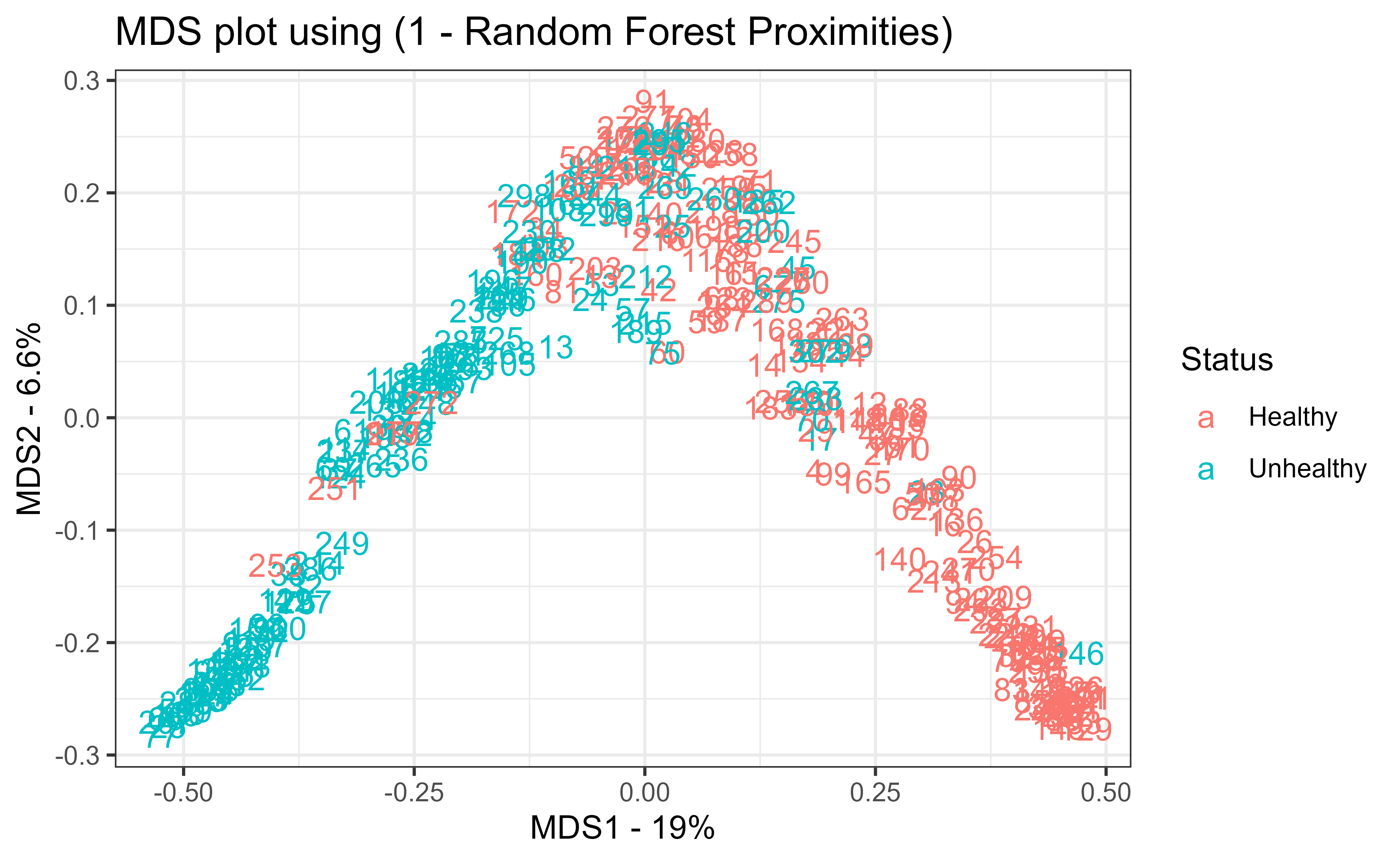
Finally, the model is refit with the best mtry and its proximity matrix is turned into a distance matrix via 1 - proximity, which feeds classical multidimensional scaling (cmdscale; see Chapter 31). Figure 13.3 shows the resulting MDS plot, which places each patient in two dimensions so that patients the forest treats as similar sit close together. Coloring by true status shows how cleanly the forest separates healthy from unhealthy patients, a visual companion to the numeric OOB error.
Show code
## Now let's create an MDS-plot to show how the samples are related to each## other.#### Start by converting the proximity matrix into a distance matrix.distance.matrix<-as.dist(1-model$proximity)mds.stuff<-cmdscale(distance.matrix, eig=TRUE, x.ret=TRUE)## calculate the percentage of variation that each MDS axis accounts for...mds.var.per<-round(mds.stuff$eig/sum(mds.stuff$eig)*100, 1)## now make a fancy looking plot that shows the MDS axes and the variation:mds.values<-mds.stuff$pointsmds.data<-data.frame(Sample=rownames(mds.values), X=mds.values[,1], Y=mds.values[,2], Status=data.imputed$hd)ggplot(data=mds.data, aes(x=X, y=Y, label=Sample))+geom_text(aes(color=Status))+theme_bw()+xlab(paste("MDS1 - ", mds.var.per[1], "%", sep=""))+ylab(paste("MDS2 - ", mds.var.per[2], "%", sep=""))+ggtitle("MDS plot using (1 - Random Forest Proximities)")# ggsave(file="random_forest_mds_plot.pdf")
Figure 13.3: Multidimensional scaling of the heart disease patients based on one minus the random forest proximities. Points the forest treats as similar sit close together, and coloring by true status shows how cleanly the forest separates healthy from unhealthy patients.
Key idea
Proximities turn a black-box ensemble into something you can see. Two observations are “close” if they often land in the same terminal nodes across the forest, so an MDS plot of 1 - proximity reveals the structure the forest has learned, including which points sit near the decision boundary.
To recap the workflow: clean and type the data, impute missing values with rfImpute, fit a forest and read its OOB error and confusion matrix, add trees until the OOB error stabilizes, tune mtry against OOB error, and finally use proximities to visualize the learned structure. The same recipe transfers to most random forest problems you will meet.
Equivalently, correlation reduces the effective degrees of freedom in the data, so an average of correlated quantities behaves like an average of fewer truly independent ones.↩︎
# Random Forests {#sec-random-forest}```{r}#| include: falsesource("_common.R")```A single decision tree is easy to read but hard to trust: change a few training points and the tree can split on a completely different variable, sending its predictions in a new direction. Trees are, in the language of the bias-variance tradeoff, low bias but high variance learners. Bagging (@sec-bagging) already addresses this by growing many trees on bootstrap resamples and averaging them, which knocks down variance without raising bias much. Random forests push that idea one step further. They start from bagging and add a single, almost embarrassingly simple twist that turns out to matter a great deal: at every split, each tree is only allowed to look at a random handful of the predictors.In this chapter you will learn why that twist works (it is a story about correlation, not about individual trees getting better), how the algorithm is put together step by step, how to read its built-in error estimate and variable-importance scores, and how to fit and tune one in R. Random forests are a strong default for general nonlinear, nonparametric prediction, so this is a method worth understanding well before reaching for anything fancier.::: {.callout-tip title="Intuition"}Bagging averages many trees, but if those trees all key on the same one or two dominant predictors, they make correlated mistakes, and averaging correlated things barely helps. Random forests force the trees to disagree by hiding most of the predictors at each split. The trees become more diverse, their errors cancel more effectively, and the average is more stable.:::## From bagging to decorrelated treesRandom forests are a bootstrap-based procedure built on a committee of trees, exactly like bagging (@sec-bagging). The difference is that random forests deliberately *decorrelate* the trees. At each split in the tree-building process, and separately for each bootstrap sample, the splitting rule is chosen from a randomly selected, relatively small subset of the input variables. Because different variables are available at different splits and in different trees, the trees stop leaning on the same dominant covariates and become much less dependent on one another. That reduced dependence is what reduces the variance of the final prediction.This variance reduction is the whole point. Trees are inherently noisy, but when grown fairly deep they have relatively low bias. Averaging many low-bias, nearly independent trees therefore gives predictions (or classifications) that keep the low bias while shedding most of the variance.To see why correlation is the villain, recall a basic fact about averaging: the variance of an average of *correlated* variables is larger than the variance of an average of the same number of *independent* variables.^[Equivalently, correlation reduces the effective degrees of freedom in the data, so an average of correlated quantities behaves like an average of fewer truly independent ones.] Concretely, the average of $B$ identically distributed random variables, each with variance $\sigma^2$ and pairwise correlation $\rho$, has variance$$\rho \sigma^2 + \sigma^2 \frac{1 - \rho}{B}$$ {#eq-random-forest-avgvar}Look at what happens as the forest grows. The second term, $\sigma^2 (1 - \rho)/B$, shrinks to zero as $B \to \infty$, but the first term, $\rho \sigma^2$, does not depend on $B$ at all. No matter how many trees you add, the variance cannot fall below this floor of $\rho \sigma^2$.### Deriving the variance of the averageIt is worth deriving @eq-random-forest-avgvar carefully, because the entire rationale for random forests rests on it. Let $T_1, \dots, T_B$ be the predictions of the individual trees at a fixed input $x$, treated as random variables over the draw of the bootstrap samples and the split randomness $\Theta_b$. Assume they are identically distributed (not independent) with common variance $\operatorname{Var}(T_b) = \sigma^2$ and common pairwise correlation $\operatorname{Corr}(T_b, T_{b'}) = \rho$ for $b \ne b'$, so that $\operatorname{Cov}(T_b, T_{b'}) = \rho \sigma^2$. The forest prediction is $\bar T = \frac{1}{B}\sum_{b=1}^B T_b$. Expanding the variance of a sum into its $B$ diagonal (variance) terms and $B(B-1)$ off-diagonal (covariance) terms,$$\operatorname{Var}(\bar T)= \frac{1}{B^2}\operatorname{Var}\!\Big(\sum_{b=1}^B T_b\Big)= \frac{1}{B^2}\Big[\sum_{b=1}^B \operatorname{Var}(T_b) + \sum_{b \ne b'} \operatorname{Cov}(T_b, T_{b'})\Big]= \frac{1}{B^2}\big[B\sigma^2 + B(B-1)\rho\sigma^2\big].$$Dividing through by $B^2$ and rearranging gives$$\operatorname{Var}(\bar T) = \frac{\sigma^2}{B} + \frac{B-1}{B}\rho\sigma^2= \rho\sigma^2 + \frac{1-\rho}{B}\sigma^2,$$ {#eq-random-forest-avgvar-derived}which is exactly @eq-random-forest-avgvar. The derivation makes the mechanism transparent: smaller $m$ removes shared dominant predictors from many splits, lowering the off-diagonal covariance $\rho\sigma^2$ and hence the irreducible floor, but pushing $m$ too small also raises each tree's own variance $\sigma^2$ and its bias, since each split now chooses from a weaker pool of candidate variables. The optimal $m$ trades these two effects off, which is why it is tuned rather than fixed.::: {.callout-note title="A subtlety about the correlation"}The relevant $\rho$ is the correlation between the predictions of two forest trees *at the same test point $x$*, induced by their shared training data, not the sampling correlation of an estimator across independent data sets. As $B$ grows, $\bar T(x)$ converges almost surely to its expectation $\mathbb{E}_\Theta[T(x;\Theta)]$ over the randomization, so $B$ is not a tuning parameter in the usual sense: more trees only ever help (up to Monte Carlo noise) and never overfit. The bound @eq-random-forest-avgvar-derived is what guarantees this.:::We can confirm @eq-random-forest-avgvar-derived numerically with a small base-R simulation. We generate $B$ correlated Gaussian variables with variance $\sigma^2$ and pairwise correlation $\rho$, average them, repeat many times, and compare the empirical variance of the average to the formula.```{r random-forest-variance-check}set.seed(1)sigma2 <-4; rho <-0.3; B <-20; reps <-20000## equicorrelation covariance: Sigma = sigma2 * [(1-rho) I + rho 11']L <-t(chol(sigma2 * ((1- rho) *diag(B) + rho *matrix(1, B, B))))means <-replicate(reps, mean(L %*%rnorm(B)))emp <-var(means)theo <- rho * sigma2 + (1- rho) * sigma2 / Bc(empirical = emp, theoretical = theo)```The two numbers agree to Monte Carlo error, and increasing `B` drives the average's variance toward the floor `rho * sigma2 = 1.2`, never below it.::: {.callout-important title="Key idea"}Adding more trees only attacks the $\sigma^2(1-\rho)/B$ part of the variance. The floor $\rho \sigma^2$ can only be lowered by reducing the correlation $\rho$ between trees. Random forests lower $\rho$ by randomizing the variables available at each split, which is precisely the dependence that plain bagging (@sec-bagging) leaves in place.:::## The algorithmBefore the formal statement, here is the idea in four plain steps:1. Create bootstrapped datasets (sampling with replacement).2. Grow a decision tree on each bootstrapped dataset, but at every split consider only a random subset of the variables.3. Repeat steps 1 and 2 many times to build a whole forest.4. To predict, run a new observation through every tree and combine the results: average them for regression, or take a majority vote for classification (the same aggregation idea as in bagging (@sec-bagging), applied to many bootstrap samples).The one new knob compared to bagging is $m$, the number of input variables made available at each split, where $m \le p$ and $p$ is the total number of predictors. Smaller $m$ means more aggressive decorrelation. There is no theory that pins down the best value, but two rules of thumb, supported by simulation studies rather than by any deeper result, work well as starting points:- $m = \sqrt{p}$ for classification.- $m = \frac{p}{3}$ for regression.After $B$ trees are grown, $\{T(x, \Theta_b)\}^B_1$, the random forest regression predictor is the simple average of the trees,$$\hat{f}^B_{rf} (x) = \frac{1}{B} \sum_{b=1}^B T(x; \Theta_b)$$where $\Theta_b$ collects the split variables and cut points of the $b$-th tree.Putting the pieces together gives the standard algorithm for both regression and classification [@hastie2001a, Alg 15.1]:1. For $b = 1$ to $B$: 1. Draw a bootstrap sample $\mathbf{Z}^*$ of size N from the training data. 2. Grow a random-forest tree $T_b$ on the bootstrapped data by recursively repeating the following steps at each terminal node, until the minimum node size $n_{min}$ is reached: 1. Select $m$ variables at random from the $p$ variables. 2. Pick the best variable and split-point among those $m$. 3. Split the node into two daughter nodes.2. Output the ensemble of trees $\{T_b\}^B_1$.To predict at a new point $x$, the two tasks differ only in how the trees are combined:- Regression: $\hat{f}_{rf}^B(x) = \frac{1}{B}\sum_{b=1}^B T_b(x)$.- Classification: let $\hat{C}_b (x)$ be the class predicted by the $b$-th tree. Then $\hat{C}_{rf}^B (x) = \text{majority vote } \{\hat{C}_b (x) \}^B_{1}$.::: {.callout-note}Random subset selection happens *at every split*, not once per tree. A fresh random set of $m$ variables is drawn each time a node is split, which is what keeps even the same tree from being dominated by one strong predictor.:::How does this compare to its neighbors? In general, gradient boosting (@sec-gradient-boosting) is roughly comparable to random forests, and random forests usually beat plain bagging (@sec-bagging), though in practice these orderings do not always hold. Which method wins depends on the structure of the problem: the degree of linearity or nonlinearity, the dependence among covariates, the relative importance of specific predictors, and so on.::: {.callout-tip title="When to use this"}Reach for a random forest when you want strong nonlinear, nonparametric prediction with little tuning, mixed variable types, and a built-in honest error estimate. If you need to squeeze out the last bit of accuracy on highly structured data, compare against gradient boosting (@sec-gradient-boosting).:::## Out-of-bag error: free cross-validationA pleasant side effect of bootstrapping is that the forest comes with its own validation set. Each bootstrap sample leaves out roughly a third of the observations, and those left-out points are called the out-of-bag (OOB) samples for that tree.For each observation pair $(x_i, y_i)$, we can form an OOB prediction by averaging only the trees built on bootstrap samples in which that observation did not appear. Comparing these OOB predictions to the actual responses gives the OOB error, which behaves like a cross-validation error estimate but costs nothing extra to compute. A useful practical signal falls out of this: once the OOB error stops improving as you add trees, the forest has effectively converged and more trees will not help.### Why roughly a third is left outThe "roughly a third" is not a heuristic; it follows from the bootstrap. A bootstrap sample draws $N$ points with replacement from a training set of size $N$, so each draw selects observation $i$ with probability $1/N$. The probability that observation $i$ is missed on all $N$ draws is$$\Pr(i \notin \mathbf{Z}^*) = \Big(1 - \frac{1}{N}\Big)^{N}\;\xrightarrow[N \to \infty]{}\; e^{-1} \approx 0.368,$$ {#eq-random-forest-oobfrac}using $\lim_{N\to\infty}(1 - 1/N)^N = e^{-1}$. Hence about $36.8\%$ of observations are out-of-bag for any given tree, and a given observation is OOB for, in expectation, a fraction $e^{-1}$ of the $B$ trees, leaving on the order of $0.368\,B$ trees to form its OOB prediction. Because the OOB prediction of $(x_i, y_i)$ uses only trees that never saw that point, the OOB error is a genuine held-out estimate of generalization error. As $B \to \infty$ it is asymptotically equivalent to leave-one-out cross-validation over the bootstrap distribution, which is why it can replace a manually held-out test set.::: {.callout-warning title="When OOB error is optimistic or unstable"}The OOB estimate degrades when the number of trees is small (each point then has very few OOB trees, so its prediction is noisy) and when observations are not independent, for example with spatial, temporal, or grouped data. In the latter case bootstrap resampling does not break the dependence between in-bag and out-of-bag points, and the OOB error can be badly optimistic, just as ordinary cross-validation is when folds share dependent records.:::::: {.callout-tip}Watch the OOB error as a function of the number of trees. When the curve flattens, you have enough trees. This is the random forest equivalent of a learning curve, and you get it without holding out a separate set.:::## Variable importanceBecause each split sees a random subset of predictors, random forests give variables that would otherwise be overshadowed a chance to be chosen. As a result, the forest tends to surface more "important" variables than a single greedy tree would. There are two common ways to score importance.The first measures, for each variable, how much it improves the split criterion (such as node impurity) summed and averaged across all trees. Variables that produce big, frequent improvements score high. Formally, let a split $s$ at an internal node $t$ send a fraction $p_L$ of the node's samples left and $p_R = 1 - p_L$ right, and let $i(\cdot)$ be the node impurity (Gini index or entropy for classification, residual sum of squares for regression). The impurity decrease at that node is$$\Delta i(s, t) = i(t) - p_L\, i(t_L) - p_R\, i(t_R),$$ {#eq-random-forest-mdi}weighted by the proportion of samples reaching $t$. The mean decrease in impurity (MDI) importance of variable $j$ is the sum of these weighted decreases over all nodes that split on $j$, averaged over the $B$ trees. MDI is essentially free, since the quantities are already computed during training, but it is biased: it inflates the apparent importance of high-cardinality categorical variables and continuous variables, which offer more candidate split points and thus more chances to reduce impurity even by chance.The second is permutation importance, which is based on OOB prediction. When the $b$-th tree is grown, its OOB samples are passed down the tree and the prediction accuracy is recorded. The values of the $j$-th variable are then randomly permuted across those OOB samples, breaking any relationship between that variable and the response, and the accuracy is recomputed. The drop in accuracy, averaged over all trees, measures the importance of variable $j$. Writing $\mathrm{OOB}_b$ for the out-of-bag set of tree $b$ and $\pi_j$ for a random permutation of the $j$-th coordinate within that set, the permutation importance is$$\mathrm{VI}(j) = \frac{1}{B}\sum_{b=1}^{B}\Big[ \mathrm{err}_b\big(\mathrm{OOB}_b^{\,\pi_j}\big) - \mathrm{err}_b\big(\mathrm{OOB}_b\big) \Big],$$ {#eq-random-forest-vi}where $\mathrm{err}_b$ is the tree's OOB error (misclassification rate or mean squared error). Because the comparison is made on held-out data with the model fixed, @eq-random-forest-vi measures how much the fitted forest actually relies on $X_j$ for prediction, which is a different and usually more trustworthy question than MDI's "how often did $X_j$ get chosen during training."::: {.callout-warning title="Correlated predictors distort both scores"}When two predictors are strongly correlated, the forest can split on either one, so neither looks individually indispensable and both can receive deflated permutation scores even though the pair is jointly important. Permuting a variable marginally also generates feature combinations that never occur in the data (extrapolation), which can make the importance unstable. Conditional permutation importance and grouped or drop-and-relearn schemes address these failure modes at higher computational cost.:::::: {.callout-warning}Permutation importance does not tell you how the model would do if that variable were simply *unavailable*. A refit model would likely lean on correlated surrogate variables to fill the gap, so dropping a "high importance" variable may hurt far less than its score suggests.:::## Other properties to keep in mindA few additional points round out the picture of how random forests behave in practice:- Proximity plots show which observations the forest treats as effectively close together. They are useful mainly for seeing where points sit relative to the decision boundary; we use this idea in the application below to build an MDS plot.- Overfitting: random forests are fairly robust to overfitting when the number of genuinely relevant variables in $X$ is large relative to $p$.- Bias: the bias of a random forest is essentially the same as the bias of an individual tree. The gain in mean squared error comes entirely from variance reduction, not from lower bias.- Relationship to other methods: a random forest behaves somewhat like a nearest-neighbor classifier (such as $k$-nearest neighbor; see @sec-knn), since predictions are driven by training points that fall in the same regions.- Software: common implementations include `randomForest`, `cforest`, `ParallelForest`, `ranger`, and `Rborist`.In short, random forests are a reliable, low-maintenance tool for general nonlinear, nonparametric prediction. With the mechanics in hand, the rest of the chapter walks through a complete worked example.## Statistical propertiesThis section collects the theoretical facts that justify the method, going beyond the variance argument of @sec-random-forest.### Bias-variance decomposition of the ensembleFix a test point $x$ and write the forest estimate as $\hat f_{rf}(x) = \mathbb{E}_\Theta[T(x;\Theta)]$ in the infinite-tree limit (averaging over the randomization $\Theta$ for a fixed training set, then over training sets). For squared-error loss the usual decomposition holds,$$\mathbb{E}\big[(Y - \hat f_{rf}(x))^2 \mid X = x\big]= \underbrace{\sigma_\varepsilon^2}_{\text{irreducible}}+ \underbrace{\big(\mathbb{E}[\hat f_{rf}(x)] - f(x)\big)^2}_{\text{bias}^2}+ \underbrace{\operatorname{Var}\big(\hat f_{rf}(x)\big)}_{\text{variance}} .$$ {#eq-random-forest-bv}Two facts make random forests work. First, averaging is a linear operation, so the bias of the ensemble equals the bias of a single randomized tree: $\mathbb{E}[\hat f_{rf}(x)] = \mathbb{E}_\Theta\mathbb{E}[T(x;\Theta)]$, and randomizing the candidate variables does not change the expected fitted function by much when trees are grown deep. This is the precise sense of the chapter's earlier remark that the forest's bias is essentially that of one tree. Second, the variance term is exactly @eq-random-forest-avgvar-derived and is driven down toward its floor $\rho\sigma^2$ by decorrelation. The entire MSE gain over a single tree comes from the variance term; the price of decorrelation is a slight increase in $\sigma^2$ and bias as $m$ shrinks, which is why very small $m$ can underperform.### Consistency and ratesRandom forests are nonparametric estimators, and consistency results require care because the bootstrap and the data-dependent splits make the trees hard to analyze. Two routes are standard. For *centered* or *purely random* forests, whose splits are chosen independently of $Y$, one can show $L^2$ consistency, $\mathbb{E}[(\hat f_{rf}(X) - f(X))^2] \to 0$, under mild smoothness of $f$, with rates governed by the effective number of cells. The convergence rate is the nonparametric rate $n^{-2/(2 + d)}$ for a $d$-dimensional Lipschitz target in the worst case, slower as $d$ grows (the curse of dimensionality), but the rate adapts to a smaller intrinsic dimension when only a few of the $p$ inputs are relevant, which is the regime where forests shine. For Breiman's original CART-split forests, whose splits depend on $Y$ and are far harder to analyze, consistency has been established under an additive-model assumption (Scornet, Biau, and Vert, 2015). The practical message is that forests are consistent under reasonable conditions but converge at nonparametric rates, so they cannot escape the curse of dimensionality when the truth genuinely depends on many interacting variables.### Connection to adaptive nearest neighbors and kernelsA forest prediction can be written as a weighted average of the training responses,$$\hat f_{rf}(x) = \sum_{i=1}^N w_i(x)\, y_i,\qquadw_i(x) = \frac{1}{B}\sum_{b=1}^B \frac{\mathbf{1}\{x_i \in L_b(x)\}}{|L_b(x)|},$$ {#eq-random-forest-weights}where $L_b(x)$ is the terminal node ("leaf") of tree $b$ containing $x$ and $|L_b(x)|$ is the number of training points in it. The weight $w_i(x)$ is large when $x_i$ falls in the same leaf as $x$ in many trees, which is exactly the proximity used for the MDS plot in the application. Equation @eq-random-forest-weights shows a random forest is an *adaptive* nearest-neighbor or kernel method: it defines a data-driven similarity $w_i(x)$ that, unlike fixed-bandwidth $k$-nearest neighbors (@sec-knn), stretches and shrinks the neighborhood along directions the trees deem relevant. This view also yields quantile and survival forests (predict a weighted quantile or weighted Kaplan-Meier curve using the same $w_i$) and underlies the infinitesimal-jackknife and U-statistic variance estimators for forest predictions.### Computational and sample complexityBuilding one tree costs $O(\tilde m\, N \log N)$ in the typical balanced case, where $\tilde m$ is the number of candidate variables evaluated per node (here $m$) and the $N \log N$ comes from sorting or scanning $N$ points down a tree of depth $O(\log N)$; the full forest is $O(B\, m\, N \log N)$. Memory is $O(B \times \text{nodes per tree})$, which can be substantial for deep trees on large $N$. Prediction costs $O(B \log N)$ per query, since each query traverses $B$ trees of depth $O(\log N)$. The trees are independent, so both training and prediction are embarrassingly parallel across the $B$ trees, which is why packages such as `ranger` scale well across cores. Reducing $m$ reduces per-node work linearly, an underappreciated reason small $m$ is fast as well as more decorrelated.### Failure modesRandom forests break or underperform in identifiable situations. They cannot extrapolate: because every prediction is a weighted average of observed $y_i$ via @eq-random-forest-weights, predictions are bounded by the range of the training responses, so a forest will systematically under- or over-predict beyond the training support and is a poor choice for strongly trending time series. They are inefficient on sparse high-dimensional problems where most of $p$ is noise, since with small $m$ a relevant variable is rarely even offered at a split; some implementations counter this with informed sampling of candidate variables. Smooth or strongly linear signals are fit with axis-aligned step functions, so a forest needs many trees to approximate a simple linear surface that a linear model captures exactly. Finally, default settings can overfit noisy classification when classes are imbalanced; class weights, stratified bootstrap sampling, or balanced subsampling are the usual remedies.## ApplicationTo make the ideas concrete, we walk through a complete classification example: predicting whether a patient has heart disease. Along the way we will impute missing values, fit a forest, read its OOB error, tune $m$ (called `mtry` in the code), and visualize the patients with a proximity-based plot. The example follows a demo by Josh Starmer^[<https://github.com/StatQuest/random_forest_demo/blob/master/random_forest_demo.R>].We start by loading the packages we need: `ggplot2` and `cowplot` for plotting, and `randomForest` for the model itself.```{r}library(ggplot2)library(cowplot)library(randomForest)```The data comes from the UCI machine learning repository^[<http://archive.ics.uci.edu/ml/index.php>], specifically the heart disease data set^[<http://archive.ics.uci.edu/ml/datasets/Heart+Disease>]. We read it directly from the URL.```{r}url <-"http://archive.ics.uci.edu/ml/machine-learning-databases/heart-disease/processed.cleveland.data"data <-read.csv(url, header=FALSE)```The raw file arrives with no column names and a few quirks, so before modeling we reformat it for two reasons: to make it easy to read by giving the columns meaningful names, and to make sure `randomForest` interprets each variable correctly (factors as factors, missing values as `NA` rather than the literal string `"?"`). The comments below document what each clinical variable means.```{r}head(data) # you see data, but no column namescolnames(data) <-c("age","sex",# 0 = female, 1 = male"cp", # chest pain # 1 = typical angina, # 2 = atypical angina, # 3 = non-anginal pain, # 4 = asymptomatic"trestbps", # resting blood pressure (in mm Hg)"chol", # serum cholestoral in mg/dl"fbs", # fasting blood sugar if less than 120 mg/dl, 1 = TRUE, 0 = FALSE"restecg", # resting electrocardiographic results# 1 = normal# 2 = having ST-T wave abnormality# 3 = showing probable or definite left ventricular hypertrophy"thalach", # maximum heart rate achieved"exang", # exercise induced angina, 1 = yes, 0 = no"oldpeak", # ST depression induced by exercise relative to rest"slope", # the slope of the peak exercise ST segment # 1 = upsloping # 2 = flat # 3 = downsloping "ca", # number of major vessels (0-3) colored by fluoroscopy"thal", # this is short of thalium heart scan# 3 = normal (no cold spots)# 6 = fixed defect (cold spots during rest and exercise)# 7 = reversible defect (when cold spots only appear during exercise)"hd"# (the predicted attribute) - diagnosis of heart disease # 0 if less than or equal to 50% diameter narrowing# 1 if greater than 50% diameter narrowing )# head(data) # now we have data and column names# str(data) # this shows that we need to tell R which columns contain factors# it also shows us that there are some missing values. There are "?"s# in the dataset.## First, replace "?"s with NAs.data[data =="?"] <-NA## Now add factors for variables that are factors and clean up the factors## that had missing data...data[data$sex ==0,]$sex <-"F"data[data$sex ==1,]$sex <-"M"data$sex <-as.factor(data$sex)data$cp <-as.factor(data$cp)data$fbs <-as.factor(data$fbs)data$restecg <-as.factor(data$restecg)data$exang <-as.factor(data$exang)data$slope <-as.factor(data$slope)data$ca <-as.integer(data$ca) # since this column had "?"s in it (which# we have since converted to NAs) R thinks that# the levels for the factor are strings, but# we know they are integers, so we'll first# convert the strings to integers...data$ca <-as.factor(data$ca) # ...then convert the integers to factor levelsdata$thal <-as.integer(data$thal) # "thal" also had "?"s in it.data$thal <-as.factor(data$thal)## This next line replaces 0 and 1 with "Healthy" and "Unhealthy"data$hd <-ifelse(test=data$hd ==0, yes="Healthy", no="Unhealthy")data$hd <-as.factor(data$hd) # Now convert to a factorstr(data) ## this shows that the correct columns are factors and we've replaced## "?"s with NAs because "?" no longer appears in the list of factors## for "ca" and "thal"```With the data cleaned and typed correctly, we are ready to build a forest. This is a good moment to recall the OOB idea from earlier in the chapter, because it changes how we set up the example.::: {.callout-note}Most machine learning methods require you to split the data manually into a training set and a test set, so you can train on one part and evaluate on data the model never saw. Random forests do this splitting for you. Because each tree is built on a bootstrap sample, not every observation is used in every tree: the bootstrap sample plays the role of the training data, and the left-out observations, the out-of-bag (OOB) data, play the role of the test set. That is why the example below never carves out a separate test set by hand.:::We also have missing values to deal with. Rather than drop incomplete rows, we impute them using `rfImpute`, which fills in missing entries based on random forest proximities (how similar observations are according to a preliminary forest). Breiman suggests 4 to 6 iterations is usually enough, so we use `iter = 6`.```{r}set.seed(42)## impute any missing values in the training set using proximitiesdata.imputed <-rfImpute(hd ~ ., data = data, iter=6)## NOTE: iter = the number of iterations to run. Breiman says 4 to 6 iterations## is usually good enough. With this dataset, when we set iter=6, OOB-error## bounces around between 17% and 18%. When we set iter=20,# set.seed(42)# data.imputed <- rfImpute(hd ~ ., data = data, iter=20)## we get values a little better and a little worse, so doing more## iterations doesn't improve the situation.#### NOTE: If you really want to micromanage how rfImpute(),## you can change the number of trees it makes (the default is 300) and the## number of variables that it will consider at each step.## Now we are ready to build a random forest.## NOTE: If the thing we're trying to predict (in this case it is## whether or not someone has heart disease) is a continuous number## (i.e. "weight" or "height"), then by default, randomForest() will set## "mtry", the number of variables to consider at each step,## to the total number of variables divided by 3 (rounded down), or to 1## (if the division results in a value less than 1).## If the thing we're trying to predict is a "factor" (i.e. either "yes/no"## or "ranked"), then randomForest() will set mtry to## the square root of the number of variables (rounded down to the next## integer value).## In this example, "hd", the thing we are trying to predict, is a factor and## there are 13 variables. So by default, randomForest() will set## mtry = sqrt(13) = 3.6 rounded down = 3## Also, by default random forest generates 500 trees (NOTE: rfImpute() only## generates 300 tress by default)model <-randomForest(hd ~ ., data=data.imputed, proximity=TRUE)## RandomForest returns all kinds of thingsmodel # gives us an overview of the call, along with...# 1) The OOB error rate for the forest with ntree trees. # In this case ntree=500 by default# 2) The confusion matrix for the forest with ntree trees.# The confusion matrix is laid out like this:```Printing the model object gives a compact summary of the fit. Two pieces matter most: the OOB estimate of the error rate (here for the default `ntree = 500` trees), which is our honest, cross-validation-like accuracy check, and the confusion matrix, which breaks the errors down by class. The confusion matrix is laid out like this, with true classes in the rows and predicted classes in the columns: Healthy Unhealthy --------------------------------------------------------------Healthy | Number of healthy people | Number of healthy people || correctly called "healthy" | incorrectly called "unhealthy" || by the forest. | by the forest | --------------------------------------------------------------Unhealthy| Number of unhealthy people | Number of unhealthy people || incorrectly called | correctly called "unhealthy" || "healthy" by the forest | by the forest | --------------------------------------------------------------Next we check whether the forest has enough trees. The principle from earlier applies directly: up to a point, more trees help, and you know you have enough once the OOB error stops improving. We plot the OOB error against the number of trees, tracking the overall rate as well as the per-class rates, so we can watch for convergence. @fig-random-forest-oob-500 shows the result for the default 500-tree forest.```{r fig-random-forest-oob-500, fig.cap="Out-of-bag error rate as a function of the number of trees for the 500-tree heart disease forest. The overall OOB rate is shown alongside the per-class rates for healthy and unhealthy patients."}## Now check to see if the random forest is actually big enough...## Up to a point, the more trees in the forest, the better. You can tell when## you've made enough when the OOB no longer improves.oob.error.data <-data.frame(Trees=rep(1:nrow(model$err.rate), times=3),Type=rep(c("OOB", "Healthy", "Unhealthy"), each=nrow(model$err.rate)),Error=c(model$err.rate[,"OOB"], model$err.rate[,"Healthy"], model$err.rate[,"Unhealthy"]))ggplot(data=oob.error.data, aes(x=Trees, y=Error)) +geom_line(aes(color=Type))# ggsave("oob_error_rate_500_trees.pdf")## Blue line = The error rate specifically for calling "Unheathly" patients that## are OOB.#### Green line = The overall OOB error rate.#### Red line = The error rate specifically for calling "Healthy" patients## that are OOB.```After building a random forest with 500 trees, the graph does not make it clear that the OOB error has settled on a value or, if we added more trees, whether it would continue to decrease. So we do the whole thing again, but this time add more trees. @fig-random-forest-oob-1000 repeats the OOB curve for a 1,000-tree forest.```{r fig-random-forest-oob-1000, fig.cap="Out-of-bag error rate as a function of the number of trees for the 1,000-tree heart disease forest. The curve flattens, showing that the OOB error has converged."}model <-randomForest(hd ~ ., data=data.imputed, ntree=1000, proximity=TRUE)modeloob.error.data <-data.frame(Trees=rep(1:nrow(model$err.rate), times=3),Type=rep(c("OOB", "Healthy", "Unhealthy"), each=nrow(model$err.rate)),Error=c(model$err.rate[,"OOB"], model$err.rate[,"Healthy"], model$err.rate[,"Unhealthy"]))ggplot(data=oob.error.data, aes(x=Trees, y=Error)) +geom_line(aes(color=Type))# ggsave("oob_error_rate_1000_trees.pdf")## After building a random forest with 1,000 trees, we get the same OOB-error## 16.5% and we can see convergence in the graph. So we could have gotten## away with only 500 trees, but we wouldn't have been sure that number## was enough.```With 1,000 trees the OOB error lands at essentially the same value as with 500 and the curve clearly flattens, confirming that 500 trees would have been enough; we just could not be sure of that until we checked. Next we tune `mtry`, the number of variables considered at each split, by sweeping it from 1 to 10 and recording the final OOB error of each forest.```{r random-forest-mtry-tuning}## If we want to compare this random forest to others with different values for## mtry (to control how many variables are considered at each step)...oob.values <-vector(length=10)for(i in1:10) { temp.model <-randomForest(hd ~ ., data=data.imputed, mtry=i, ntree=1000) oob.values[i] <- temp.model$err.rate[nrow(temp.model$err.rate),1]}oob.values## find the minimum errormin(oob.values)## find the optimal value for mtry...which(oob.values ==min(oob.values))## create a model for proximities using the best value for mtrymodel <-randomForest(hd ~ .,data=data.imputed,ntree=1000,proximity=TRUE,mtry=which(oob.values ==min(oob.values)))```The loop over `mtry` from 1 to 10 refits the forest for each candidate number of variables per split and records its final OOB error, then picks the value with the lowest error. This is how we tune $m$ in practice rather than relying only on the $\sqrt{p}$ rule of thumb.::: {.callout-tip}The `mtry` loop is a small grid search over the one knob that distinguishes a random forest from bagging. Because OOB error is nearly free, sweeping `mtry` is cheap and often worthwhile, especially when predictors are correlated and the default may be too large or too small.:::Finally, the model is refit with the best `mtry` and its proximity matrix is turned into a distance matrix via `1 - proximity`, which feeds classical multidimensional scaling (`cmdscale`; see @sec-scaling). @fig-random-forest-mds shows the resulting MDS plot, which places each patient in two dimensions so that patients the forest treats as similar sit close together. Coloring by true status shows how cleanly the forest separates healthy from unhealthy patients, a visual companion to the numeric OOB error.```{r fig-random-forest-mds, fig.cap="Multidimensional scaling of the heart disease patients based on one minus the random forest proximities. Points the forest treats as similar sit close together, and coloring by true status shows how cleanly the forest separates healthy from unhealthy patients."}## Now let's create an MDS-plot to show how the samples are related to each## other.#### Start by converting the proximity matrix into a distance matrix.distance.matrix <-as.dist(1-model$proximity)mds.stuff <-cmdscale(distance.matrix, eig=TRUE, x.ret=TRUE)## calculate the percentage of variation that each MDS axis accounts for...mds.var.per <-round(mds.stuff$eig/sum(mds.stuff$eig)*100, 1)## now make a fancy looking plot that shows the MDS axes and the variation:mds.values <- mds.stuff$pointsmds.data <-data.frame(Sample=rownames(mds.values),X=mds.values[,1],Y=mds.values[,2],Status=data.imputed$hd)ggplot(data=mds.data, aes(x=X, y=Y, label=Sample)) +geom_text(aes(color=Status)) +theme_bw() +xlab(paste("MDS1 - ", mds.var.per[1], "%", sep="")) +ylab(paste("MDS2 - ", mds.var.per[2], "%", sep="")) +ggtitle("MDS plot using (1 - Random Forest Proximities)")# ggsave(file="random_forest_mds_plot.pdf")```::: {.callout-important title="Key idea"}Proximities turn a black-box ensemble into something you can *see*. Two observations are "close" if they often land in the same terminal nodes across the forest, so an MDS plot of `1 - proximity` reveals the structure the forest has learned, including which points sit near the decision boundary.:::To recap the workflow: clean and type the data, impute missing values with `rfImpute`, fit a forest and read its OOB error and confusion matrix, add trees until the OOB error stabilizes, tune `mtry` against OOB error, and finally use proximities to visualize the learned structure. The same recipe transfers to most random forest problems you will meet.